IEEE TRANSACTIONS ON VISUALIZATION AND COMPUTER GRAPHICS, MANUSCRIPT ID
1
A Visual Inquiry System for Space-Time and Multivariate Patterns (VIS-STAMP) Diansheng Guo*, Jin Chen, Alan M. MacEachren, and Ke Liao, *Member, IEEE Abstract—The research reported here integrates computational, visual, and cartographic methods to develop a novel geo-visual analytic strategy for exploring and understanding spatio-temporal and multivariate patterns. The developed methodology and tools can cluster, sort, and visualize large datasets and help analysts investigate complex patterns across multivariate, spatial, and temporal dimensions. Specifically, the approach involves a self-organizing map, a parallel coordinate plot, several forms of reorderable matrices (including several ordering methods), a novel geographic small multiple display, and a 2-dimensional cartographic color design method. Novel coupling among these methods leverages their independent strengths and facilitates a visual exploration of patterns that are difficult to discover otherwise. The visual inquiry system we developed supports overview of complex patterns and, through a variety of interactions, enables users to focus on specific patterns and examine detailed views. We demonstrate with an application to the IEEE InfoVis 2005 Contest data set, which contains time series, geographically referenced data for companies in the U.S. Index Terms—Information visualization, multivariate and spatio-temporal visualization, self-organizing map (SOM), visual analytics, ordering, small multiples
—————————— ——————————
1 INTRODUCTION
L
ARGE datasets that contain geographic locations, time series, and multiple variables have become a common but underutilized resource in many domains, from environmental science, through business, to homeland security. Such data hold great potential to provide valuable and previously unknown information that can advance our understanding of complex phenomena and systems [3], [10], [15]. However, visualization and data mining of spatio-temporal data are challenging problems. Existing data analysis approaches, including both visual and analytical ones, have limited ability to explore large datasets across all dimensions (i.e., geographic, temporal, and multivariate spaces). The research reported here focuses on developing a geovisual analytic approach to explore multivariate spatiotemporal data, discover interesting and unknown complex patterns, and present them in an easy-to-understand form to support human interpretation, analytical reasoning, and/or decision-making. Our new approach integrates visual and computational methods to construct an overview of major patterns present in the data. Such an overview allows the analyst to perceive complex patterns across all dimensions and then guides user interactions to explore specific patterns in detail. We demonstrate an application of the approach (and resulting tools) to analysis of the changing characteristics of U.S. industries. The integrated methods and tools we present are able to: perform multivariate clustering and abstraction (including time-series clustering) with a Self Organizing ————————————————
• Diansheng Guo and Ke Liao are with the Department of Geography, University of South Carolina, 709 Bull Street, Columbia, SC 29208. E-mail:
[email protected];
[email protected]. • Jin Chen and Alan M. MacEachren are with the GeoVISTA Center, Department of Geogrpahy, Pennsylvania State University, 302 Walker, University Park, PA 16802. E-mail: {jxc93, maceachren}@psu.edu.
Map (SOM); encode the SOM result with colors derived from our ColorBrewerPlus component, which produces a twodimensional diverging-diverging color scheme; visualize the multivariate patterns with an enhanced Parallel Coordinate Plot (PCP) display, which serves as a multivariate “legend” in the integrated system; visualize the spatio-temporal variations of multivariate patterns, or the space-variable variations of temporal patterns in a hierarchical, computationally sortable matrix and a temporally or geographically ordered map matrix; and support human interactions to explore patterns from different perspectives and at different detail levels. The remainder of the paper is organized as follows. Section 2 gives a review of related research. We introduce our approach to the visualization of spatio-temporal and multivariate patterns in section 3. Section 4 demonstrates the variety of interactions that our system supports. We then briefly introduce an interesting extension to visualize spatial interaction data (e.g., companies that relocated from one state to another) in section 5. Lastly, we conclude with discussions on the advantages and limitations of the approach.
2 RELATED WORK Our integrated geo-visual analytic approach directly addresses challenges delineated in the recent research agenda for visual analytics [45] and draws upon research in several related domains. Below, we briefly review four domains upon which we build most directly: multivariate visualization, multivariate and temporal mapping, visualization of very large datasets, and computational ordering of multivariate data.
Manuscript received November 28, 2005. xxxx-xxxx/0x/$xx.00 © 200x IEEE
under review -- please do not distribute
2
IEEE TRANSACTIONS ON VISUALIZATION AND COMPUTER GRAPHICS, MANUSCRIPT ID
2.1 Multivariate Visualization
2.3 Visualization of Very Large Datasets
Multivariate visualization methods range from commonly used information graphics (e.g., tables, histograms, scatter plots, and charts [23]) through a suite of techniques introduced in the exploratory data analysis and information visualization literature, e.g., scatterplot matrices [1], matrix permutation [37], glyph [40], pixel-oriented approaches [29], and parallel coordinate plots (PCP) [24]. There is also research that combines traditional bar charts with pixel-based techniques to visualize large amounts of data with categorical and numerical types [28]. Due to display space limitations, multivariate data are often projected to a lower dimensional space using dimensional reduction techniques, e.g., multidimensional scaling [48], [50], principle component analysis (PCA), RadViz spring visualization [8], or other projection pursuit methods [11], [50]. It is impractical to provide a comprehensive review of the range of multivariate visualization methods here, thus the reader is directed to a recent paper [31] that provides a categorization of both data types and visualization methods, with illustrations of most of the methods cited above and as well as others.
Large datasets can cause serious problems for most visualization techniques and these problems can be divided into two groups: the computational efficiency problem and the visual effectiveness problem. Computational efficiency concerns the time needed to process data and render views. A visualization technique has to be computationally efficient and scalable with very large datasets to allow human interactions (e.g. [39]). The visual effectiveness problem concerns the usefulness of data views in revealing patterns. With a large dataset, data items can overlap in the visual display (e.g., points overlap in scatter plots or line segments overlap in a parallel coordinate plot PCP) and make patterns very hard (if possible at all) to perceive [29]. Enhancements to address the visual effectiveness problem have been proposed along two primary directions. One direction is to resolve the overlap in the attribute space or geographic space by sampling, density mapping [26], or repositioning (or shifting) data points [32]. Another direction is to reduce the data size by performing data abstraction (e.g., clustering or aggregation) first so that the visualization component only needs to visualize a relatively small number of data clusters instead of all individual data items, while providing drill-down capabilities that support details for selected clusters [21], [22], [46]. We take the latter approach— data abstraction with drill down—in this research.
2.2 Multivariate and Temporal Mapping Mapping is essential in visualizing geographic patterns. Multivariate mapping has long been a challenging and interesting research problem. Three primary approaches have been used: 1) multivariate representation that depicts each dimension (variable) independently through some attribute of the display and then integrates all variable depictions into one map using composite glyphs, attributes of color, or other methods [12], [17], [19], [49], [53]; 2) dimension reduction that projects multivariate information to two (or three) dimensions and then map the result (e.g., [21]), and 3) multiple linked views that show one (or more) variables per view [2], [14], [36], [38]. Subsequent efforts have focused on integration across these approaches and/or their extension through coupling with statistical and/or computational methods. Carr, White, and MacEachren [9], for example, presented a visualization approach for multivariate data analysis called conditioned choropleth maps (CCmaps) that uses a twoway layout of maps (and matching views of statistical distributions) designed to facilitate comparisons by showing the association between a dependent variable, as represented in a classed choropleth map, and two potential explanatory variables. Guo, et al [21] propose a visualcomputational approach designed to detect and visualize multivariate spatial patterns by combining multivariate clustering, multivariate visualization, and a geographic map to present a holistic view of multivariate spatial patterns. When time is a key attribute in the data analysis, strategies applied to understanding the time component include sequencing methods (either animated or interactive) and three-dimensional approaches where time is visualized as the third dimension over a two-dimensional map [34], [35]. However, both approaches have limited ability to visualize multivariate patterns across time. In this research, we combine multivariate abstractions and matrix views to visualize spatial-temporal trends of multivariate patterns or spacevariable variations of temporal patterns.
2.4 Ordering in Visualization and Data Mining Ordering is widely used in visualization techniques to accentuate patterns. For example, in the visualization of bacterial genomes, pixel arrangement is used to place adjacent nucleotides as close to each other as possible and thus to help bring out data patterns that otherwise would be difficult to perceive [51]. Ordering is also used in arranging the layout of treemaps [43]. Friendly and Kwan presented a general framework for ordering information in visual displays (tables and graphs) according to the effects or trends. Their framework can be applied to the arrangement of unordered factors for quantitative data and frequency data, and to the arrangement of variables and observations in multivariate displays (e.g., star plots, parallel coordinate plots) [16]. The concept of a reorderable matrix [6], [7], [47], as a data table visualization method, has been the focus of several recent research efforts from different perspectives, e.g. testing ordering heuristics for an interactive tool [44], and visualizing time-varying data [41]. Ordering approaches are also used to enhance visualization by re-arranging the order of dimensions or selecting a subset of dimensions based on the ordering [20], [42], [52]. In this research, we develop a reorderable matrix and a reorderable map matrix to visualize a spatio-temporal and multivariate data cube.
3 VIS-STAMP: A VISUAL-COMPUTATIONAL APPROACH Our geo-visual analytic strategy and the implemented visual inquiry system for space-time and multivariate patterns (VIS-STAMP) is a novel integration of a suite of visual, computational, and cartographic methods, which together are used to construct an overview of major patterns present under review -- please do not distribute
GUO ET AL.: A VISUAL INQUIRY SYSTEM FOR SPATIO-TEMPORAL AND MULTIVARIATE PATTERNS (VIS-STAMP)
in the data and support a variety of user interactions to assist the analyst in exploring and interpreting complex spatio-temporal patterns. Specifically, we integrate a self-organizing map (SOM) [33] to perform multivariate clustering, sorting, and coloring; a parallel coordinate plot (PCP) to visualize multivariate patterns and serve a “legend” in the integrated system; a reorderable matrix to organize multivariate patterns in the spatio-temporal space; and a reorderable map matrix to reveal spatial variation of multivariate patterns. We use logically constructed, two-dimensional color schemes to encode the SOM result and use two linear ordering methods to reorder the matrices to accentuate patterns. Our approach inherently supports both overview and detail analysis. We present the overview and its related methodology in this section and introduce user interactions that lead to detailed views in section 4.
3.1 Conceptual Data Representation To simplify the presentation of our methodology, we conceptually represent the data as a data cube (Fig. 1: A), which is defined by three components: the geography (e.g., US states), the time (e.g., years), and a set of numerical variables. Each cell in this cube is defined by a specific spatial object (e.g., Texas), a specific time (e.g., year 2000), and a specific variable (e.g., sales percentage for the energy industry). The value for that cell is the variable value. Each spatial object (e.g., Texas) has a horizontal slice in the cube, which we call a time-attribute slice (Figure 1: B). A timeattribute slice can be seen as a series of multivariate profiles (one for each year—Fig. 1: C), or a set of time series (one for each variable—Fig. 1: D). For example, suppose we construct a data cube with 50 US states, 16 industries as variables, across 12 years. Then there are 50 time-attribute slices (one for each state), 600 multivariate profiles (one for each state/year combination), and 800 time series (one for each state/industry combination). From now on, we will directly refer to these three terms without explanation. Such a space-time-attribute data cube is often an aggregation of a more detailed dataset. For example, the US company dataset that we use for demonstration in this paper is from the IEEE InfoVis 2005 Contest [18] and has 563,000+ records. Each record contains the information for a specific company at a specific year, including its location (state name and zipcode), industry type, primary product type, sales, and employees. One possible aggregation of this dataset into a data cube is to group data by state, year, and industry type. The value for each cell can be, for example, the sales value for
Fig. 1. The Spatio-temporal and multivariate data cube (A), which can be decomposed into a set of time-attribute slices (B), multivariate profiles (C), or time series (D).
3
that state/year/industry combination (e.g., California, at 2000, for computer hardware industry). The implementation of our approach allows the user to change the cube configuration interactively, e.g., using product types instead of industry types, or using employees instead of sales values. To help the reader understand our example analyses, here we briefly introduce the US company data that we use in this paper. We focus on 49 US states, including DC but excluding Hawaii and Alaska for presentation clarity, since including those two states will make other states much smaller in maps. The data span across 12 years, from 1992 to 2003. We select 16 industry types: factory automation (AUT), biotechnology (BIO), chemicals (CHE), computer hardware (COM), defense (DEF), energy (ENR), environmental (ENV), manufacturing equipment (MAN), advanced materials (MAT), medical (MED), pharmaceuticals (PHA), computer software (SOF), subassemblies and components (SUB), telecommunications and internet (TEL), transportation (TRN), and notprimarily-high-tech (NON). This dataset and its metadata are available at the IEEE InfoVis 2005 Contest website [18].
3.2 Multivariate Clustering and Visualization 3.2.1 Abstraction and Encoding of Multivariate Patterns We use a self-organizing map (SOM) to process all multivariate profiles (Fig. 1: C) and group similar multivariate profiles into clusters (nodes). More importantly, the SOM orders clusters (nodes) in a two-dimensional layout so that nearby clusters (nodes) are similar (in the multivariate space). Thus, the SOM effectively transforms the multivariate data into a twodimensional space. We then use a systematically designed two-dimensional color scheme to assign a color to each SOM node so that nearby (and therefore similar) nodes have similar colors. Below we briefly introduce this color-coded SOM. Readers are referred to a recent paper [21] for details. Our implementation of the SOM uses a traditional hexagonal layout and normally has 9x9 or less nodes (clusters) since it is difficult to construct a two-dimensional color scheme with more than 9 x 9 = 81 colors and grouping data into more clusters is seldom a sufficient abstraction to be useful. SOM clusters are visualized using a U-Matrix (Kohonen 2001) with several new added features (Fig. 2: right). Each cluster, which contains one or more data items, is depicted with a circle, whose size (area) is linearly scaled and proportional to the number of data items it contains. Each hexagon is shaded (in shades of gray) to show the multivariate dissimilarity between immediate neighboring nodes, with darker colors showing greater dissimilarity. Thus, the shaded U-Matrix reveals the non-linear mapping between the multivariate space and the regular 2D layout of nodes, which are not evenly distributed in the multivariate space. Our two-dimensional diverging-diverging color scheme (Fig. 2) uses a systematic variation in both hue and lightness to provide a 2D array of logically ordered but discriminable colors. The color scheme is derived following several steps: (1) lay a square grid net on the CIELAB AB plane; (2) elevate the grid net vertically to a surface of a geometric object (e.g., a bell shape as shown in Fig. 2); (3) rotate the elevated net (horizontally) and/or shift it (horizontally or vertically) if needed; under review -- please do not distribute
4
IEEE TRANSACTIONS ON VISUALIZATION AND COMPUTER GRAPHICS, MANUSCRIPT ID
Fig. 2. The two-dimensional color model (left) and the color-encoded SOM (right). The 2D array of colors are derived from the 2D color model, which horizontally rotates the bell-shaped mesh 25 degree clockwise and then samples a color at each knot on the mesh. See [21] for details on the color design interface. Each circle in the SOM represents a non-empty node and the area is linearly scaled and proportional to the number of data items contained in that cluster.
(4) sample colors at the grid intersections in the 3D CIELAB color space. This 2D color scheme differs from the color scheme proposed by Kaski, et al [27] in that it has more color variations to depict dissimilarities and makes the ordered sequence more clear. The size of the 2D color array is always the same as the size of the SOM. For example, if we train a SOM with 5 x 5 = 25 nodes, we will also construct a 5 x 5 array of colors (see Fig. 2). The two-dimensional array of colors is then folded onto the regular 2D layout of the SOM nodes (not onto the regression surface in the actual data space). Thus, each node corresponds to a unique color in the color array. As mentioned earlier, although the SOM nodes are ordered on a regular 2D layout, they are not evenly distributed in the multivariate data space and the distances (dissimilarities) between neighboring nodes may vary. Therefore, the color differences only represent relative dissimilarity between two clusters of data items. Caution therefore, must be exercised in the comparison of colors.
3.2.1 Visualization of Multivariate Patterns The meaning of the colors in the SOM (Fig. 2), however, cannot be defined by a simple legend (as it might be on a typical geographic map), since each color represents a multivariate cluster. Thus, the colors, which signify the relative similarity of clusters, must be supplemented by a multivariate visualization method that allows analysts to understand the characteristics of each cluster and thus the meaning of each color. To accomplish this, we extend an earlier version of a parallel coordinate plot (PCP), introduced in [21], to visualize the data clusters identified by the SOM. The previous version of the PCP visualizes clusters instead of original data items, and thus partially avoids the overlap problem. Each string (representing a cluster) has the same color as it does in the SOM, which in turn dramatically improves the visual effectiveness of PCP in presenting multivariate patterns. The PCP also uses a nestedmeans scaling on each axis and thus further alleviates the overlapping problem. Nested-means is a non-linear scaling method that recursively calculates a number of mean values (and sub-means) and uses these values as break points to divide each axis into equal-length segments. Therefore, nestedmeans scaling always puts the mean value at the center of
Fig. 3. Each string in the PCP is a cluster of multivariate profiles (i.e., industry compositions) and is colored by the SOM (see Fig. 5: bottomright). Each axis is scaled using the nested-means method, which always puts the mean value of a variable at the center of its axis. Each variable is the sales value for an industry for a state and year as a percentage of the total sales of all six selected industries for that state/year. The thickness of each string represents the number of data items contained in that cluster.
each axis and thus makes axes defined by different units and data ranges comparable (Fig. 3). We extend the earlier version of the PCP by adding features to support user interaction and information inquiry at different levels. Bertin defined three “levels of reading”, i.e., the elementary level (allowing users to view the information about a single data element), intermediate level (revealing summary information about a group of elements), and global level (presenting an overall picture of all items in the data) [6]. As shown in Fig. 3, the colored PCP at the cluster level presents a global view of the overall patterns. A user can then select one or more clusters in the PCP (or the SOM), switch to the data item level (instead of the cluster level), and examine all the data items in the cluster(s) (Fig. 4). Selection can be made on either data item or cluster level. For example, one can show data at the item level in the PCP and then select a single data item to read its exact variable values. One can also switch back to the cluster level and see which cluster the selected item belongs. That cluster may contain many other items as well—thus its circle will become a wedge to
Fig. 4. The dark green cluster that has the highest percentage for SUB industry in the PCP above (Fig. 3) is selected and shown at the data item level. We now see all the data items contained in that cluster. The scaling of each axis is also changed to global min-max.
under review -- please do not distribute
GUO ET AL.: A VISUAL INQUIRY SYSTEM FOR SPATIO-TEMPORAL AND MULTIVARIATE PATTERNS (VIS-STAMP)
show the partial selection. We demonstrate these interaction features in section 4. In addition to the nested-means method, the new version of PCP also supports several other scaling methods, including data min-max scaling—using the minimum and maximum data values to linearly scale each axis; cell min-max scaling—using the minimum and maximum cluster (node) mean values to linearly scale each axis, and global min-max scaling—using the minimum and maximum for all variable values to linearly scale each axis. The global min-max scaling is especially useful when the values on different axes are directly comparable, for example, percentage values as used in this research (Fig. 4).
5
able matrix, when one of the two dimensions represents geography, will be accompanied with a reorderable map matrix. Below we first introduce the two matrices and then introduce the ordering methods used to reorder the matrices.
3.3.1 Reorderable Matrix and Map Matrix
The reorderable matrix we implemented supports computational sorting of both columns and rows. In the application shown in Fig. 5 (top-left), columns represent time (years) and rows represent places (states of the U.S.). Ordering of time is fixed (for these applications) in normal temporal order. Ordering of places is computationally derived with several clusterbased ordering methods, which we present in the next subsection. Users can interactively choose any of the implemented 3.3 Spatio-Temporal Visualization of Multivariate sorting methods to reorder the rows. After the re-ordering, Patterns states that have similar industry patterns over time are next to The SOM and PCP together can visualize and present multi- each other in the matrix and thus form homogeneous spatiovariate patterns effectively. However, these multivariate pat- temporal “regions”. terns often vary over the geographic space and evolve over The reorderable map matrix we implemented essentially time. It is critical to visualize the data cube across all dimen- converts each column in the reorderable matrix to a map and sions (i.e., space, time, and multiple variables) and construct a these maps are arranged in the same order as that of the colholistic view of patterns present in the data cube. We develop umns (Fig. 5: top right). The advantage of a map matrix over a form of reorderable matrix to organize multivariate patterns a reorderable matrix is that the spatial topology is preserved (represented with colors) across time and space. This reorder- and it can better support the perception of spatial distribution patterns. However, the disadvantage is that the temporal trend for a specific spatial object (e.g., California) is not as clear as in the reorderable matrix. The data used in the snapshot shown in Fig. 5 includes six industry types, which are selected for demonstration— a more complete analysis with 16 industry types is included in section 4. Each cell in the reorderable matrix or a state in a map has a multivariate profile, which is a vector of sales values for the six industries (for that state/year). Then each profile is converted to percentages, i.e., each value in the vector is divided by the vector total. The SOM takes all multivariate profiles (in percentage values) as input, groups similar profiles into clusters, and assigns each cluster (and each multivariate profile) a color. Similar colors represent similar profiles. Therefore, both the reorderable matrix and the map matrix are actually “3D” views of the data cube, showing information across space (represented with the vertical dimension in the spatio-temporal matrix or with maps in the map matrix), time (represented with the horizontal dimension), and multiple variables (represented by colors). In the middle of the reorderable matrix as depicted in Fig. 5, for example, Fig. 5. The reorderable matrix (top-left), map matrix (top-right), multivariate “legend”—PCP we notice a “region” of purple colors (bottom-left), and the SOM (bottom-right). The states (on the vertical dimension in the reorderable matrix) are ordered with complete-linkage ordering (see next section). The meaning for and it contains Louisiana (LA), Okalacolors, which represent industry compositions, can be interpreted from the PCP. In this snaphoma (OK), and Texas (TX), across all shot, each axis in the PCP is scaled using nested-means and each string represents a SOM years (except Texas and Okalahoma at cluster. The thickness of each string is lindearly scaled to show the cluster size. under review -- please do not distribute
6
IEEE TRANSACTIONS ON VISUALIZATION AND COMPUTER GRAPHICS, MANUSCRIPT ID
1992). From the PCP we understand that purple colors signify industry compositions dominated by the energy industry (ENR). Similarly, we also notice a dark red “region” (right above that purple “region”) consisting of four states: Washington DC for 1992-1997, Arkansas (AR) for 1992-1999, New Mexico (NM) for 1994-2000, and Missouri (MS) for 1995-2003. From the PCP we know that dark red or red colors represent a high percentage of the telecommunication and internet industry (TEL). We also see that, around the late 90s, three of those red states (except Missouri) changed to not-primarily-high-tech (NON) industry (represented with blue colors). Another overall pattern we can easily perceive is that many states shifted to the NON industry (represented by blue colors) since 2001. This pattern is evident in both the reorderable matrix and the map matrix. It may be related to the recession around 2000 and the nation’s focus on homeland security since 2001. Such an overview, prepared by the clustering, coloring, and ordering methods and presented with the four visual components, is a rich and yet clear representation of the major spatio-temporal and multivariate patterns present in the data cube. Even without user interactions, one can still perceive, interpret, and understand a variety of patterns by visually examining and linking those four views. Thus, it can allow the presentation and communication of complex patterns in static forms, e.g., images or printed papers, when interactive presentation is not possible.
3.3.2 Hierarchical Clustering and Matrix Ordering
Fig. 6. The two dendrograms represent the same cluster hierarchy of the five objects but the right dendrogram gives a better ordering.
simple, fast, and yet satisfying ordering strategy based on a hierarchical clustering result. Given a dendrogram (Fig. 6: middle), we process the hierarchy from the bottom up. At the beginning, each cluster contains a single item (e.g. a state). When two clusters are merged into one, the closest (i.e., most similar) ends of the two clusters should be connected. For example, when B is merged with cluster {C, D}, B should be next to D because it is closer to D than to C (Fig. 6: left). When cluster {A, E} is merged with cluster {B, D, C}, C and E should be next to each other since CE is the closest among the four connection options: AB, AC, BE, and CE. Once all data items are in the same cluster, an ordering is achieved (Fig. 6: right). Theoretically, any hierarchical clustering method can be combined with the above ordering strategy to derive a unique ordering. We implement two orderng methods, one based on the single-linkage hierarchical clustering (of O(nlogn) complexity) and the other based on the completelinkage clustering (of O(n2logn) complexity) [25]. Fig. 7 shows three reorderable matrix views of the same data (as used in Fig. 5), one is not ordered, one ordered with the single-linkage method, and the third ordered with completelinkage ordering. Generally, the complete-linkage ordering produces a slightly better result. The matrix provides flexibility to incorporate other similarity measures since similarity definitions are often application dependent. The matrix also includes a programming interface that supports connection
In this section, we introduce the ordering methods that we developed to order the matrix rows (or columns). Let A = {a1, a2, …, an} be a set of objects (either all the rows or all the columns in the matrix). All pair-wise dissimilarity values within A form a symmetric matrix (hereafter dissimilarity matrix). In this paper, we simply define the dissimilarity between two spatial objects as the Euclidean distance between their time-attribute slices (see Fig. 1), each of which is a 2D array of numerical values. To render the display of the reorderable matrix shown in Fig. 5, all rows (i.e., US states) are ordered according to their dissimilarity matrix. There are several existing methods for sorting a matrix based on dissimilarity or other measures [4], [5], [16], [20]. Here we develop an ordering strategy based on hierarchical clustering. The ordering is constrained by the hierarchical cluster structure (represented with a dendrogram—see Fig. 6), i.e., a cluster (at any level in the hierarchy) should occupy a contiguous region in the ordering. As seen in Fig. 6, however, a cluster hierarchy cannot determine a unique ordering (Fig. 6). We can derive 2n-1 (n is the number of objects to be ordered) unique orderings from the same cluster hierarchy. Bar-Joseph et al. [5] proposed a method to find the shortest one among the 2n-1 orderings, which is of O(n4) Fig. 7. A comparison of two ordering methods. The matrix on the left is not ordered (i.e., complexity and thus is not efficient enough to in alphabetical ordering). The matrix in the middle is ordered using single-linkage ordering, while the matrix on the right is ordered using complete-linkage ordering. The dissupport a highly interactive visualization ensimilarity between two rows (i.e., states) is the Euclidean distance between their timevironment. We propose and implement a attribute slices, each of which is a 2D array of numerical values. under review -- please do not distribute
GUO ET AL.: A VISUAL INQUIRY SYSTEM FOR SPATIO-TEMPORAL AND MULTIVARIATE PATTERNS (VIS-STAMP)
7
with other sorting methods. An interesting advantage here is that we can crosscheck the ordering result and the SOM result (i.e., colors) since they are constructed independently. From the matrices shown in Fig. 6, we can see that the ordering and the SOM result match very well as rows with similar colors (which is the SOM result) are also ordered next to each other (which is the result of the ordering).
3.4 Space-Variable Visualization of Temporal Patterns Our system has the flexibility to present patterns in the space-timemultivariate data cube from different perspectives. For example, we can use industry types and states to organize the reorderable matrix (now we call it space-variable matrix). In other words, each column represents an industry type and each row represents a US state. Temporal series will be treated as multivariate vectors and clustered (and colored) by the SOM. To characterize a temporal trend, we Fig. 8. Spatial distribution and industry-by-industry variation of temporal trends. Both the rows and convert each time series (one for each columns are ordered using the complete-linkage ordering method. The maps in the map matrix also state/industry combination) to per- follow the same order as that of the columns in the reorderable matrix. centages, e.g., the percentage of one matrix shows us the spatial distribution and regional differyear’s sales against all-year total for that state and industry. Now we are able to examine the variation of temporal ences in the growth of each industry. For example, the matepatterns across geography and multiple categories (e.g., in- rial industry (MAT—the third map on the top row in the dustry types) (Fig. 8). The colors represent similar temporal map matrix) had a recent growth in the northwest region, trends. From the PCP (as the legend), we can tell that green while rising sales of the manufacturing industry (MAN—the colors represent trends that peaked in the early 90s but de- second map on the last row)—focused on the Midwest and clined since then. Blue colors represent a combination of ris- east coast. With such an ordered overview of temporal patterns, oring trends in earlier years and declining trends for recent ganized spatially and industry by industry, we can decipher years. Purple colors represent a rise during 1998—2001 and a a rich set of patterns, across different states/regions, different decrease in 2002 and 2003. Red and dark red colors represent industries, and different years. a most recent growth in sales—with low sales for most years but rapid rises in 2003. Both the columns and the rows of the space-variable ma- 4 HUMAN INTERACTIONS WITH VIS-STAMP trix are ordered, separately, with the complete-linkage orderIn addition to constructing a holistic view of patterns in the ing. Patterns in the space-variable matrix (Fig. 8: top-left) are spatio-temporal and multivariate data cube, VIS-STAMP not as clear as we saw in Fig. 5. This indicates that it is rare also supports a variety of human interactions that allow the for two states to have similar temporal trends for each indusanalyst to examine patterns in detail. We specifically design try type, and that it is also rare for two industries to develop and implement the system to support three main interacin the same way in all states. However, we do see that after tion features. First, each visual component should be able to the ordering red columns are shifted to the right side in the support user selections and the selection made in one comreorderable matrix and accordingly “hot” maps are shifted to ponent should be highlighted in all other components sithe lower part in the map matrix. That gives us a clear permultaneously. Second, the user can make a selection in one ception of the industries that had rising sales in recent years component and then refine that selection in the same or and the states that those rapid increases occurred. For examanother visual component by adding or subtracting new ple, four industries had a signifant growth recently almost selection(s). Third, each component should be able to renationwide, including the telecommunication and internet spond to selections made at different levels (i.e., data ele(TEL), biotechnology (BIO), energy (ENR) and the nonments or clusters). We demonstrate such user interactions primary high-tech (NON) industry. The reorderable map with an application to the US company data, which has under review -- please do not distribute
8
IEEE TRANSACTIONS ON VISUALIZATION AND COMPUTER GRAPHICS, MANUSCRIPT ID
been used in previous analyses. Three examples are included to demonstrate interactions at three different levels, which correspond to Bertin’s three reading levels, i.e., the elementary level, intermediate level, and the global level [6].
4.1 Overview of Patterns Fig. 8 shows an overview of patterns in the US company data. There are two major differences between this analysis and the one presented in Fig. 5. First, this analysis includes 16 industry types instead of six. Please refer to section 3.1 for a list of these industries. Second, the reorderable matrix is organized into five geographic regions, i.e., the Pacific (Pac), Southwest (SW), Midwest (MID), Northeast (NE), and the Southeast (SE). The matrix supports such concept hierarchies for both the columns and rows (section 5 has another example). States (rows) in each region are Fig. 9. This is an overview of spatio-temporal and multivariate patterns of sales in the company data, which includes 16 industry types for 49 states (including DC) and 12 years. The states (on the vertical then ordered with complete- dimension in the reorderable matrix) are grouped into geographic regions and the states in each relinkage ordering according to gion are ordered with the complete-linkage ordering method. their time-attribute similarities. From this overview, we can perceive a variety of pat- 1994 Nevada’s industry sales were primarily from the energy terns across the multivariate space, time, and geography. industry (ENR) (>40%). Then, for 1995-2000, energy percentThose patterns identified in Fig. 5 are still evident here, al- ages dropped to 25% while computer hardware (COM) inthough with different colors. We also see many new pat- creased to about 40-50%. For this same period, Nevada also terns, as more industries are included in this overview. For had a moderate growth for subassemblies and components example, from the PCP we understand that the white color (SUB). Since 2001, however, Nevada’s industry sales were represents high percentages (>30%) for Advanced Materials dominated by not-primarily-high-tech (NON) type (>60%), (MAT) and from the reorderable matrix (and/or the map with only a small share from computer hardware (COM) and matrix) we can see that MAT industry dominated in West telecommunication/Internet (TEL) (about 10% each). Virginia (WV) since 1993, Utah (UT) for 1999-2002, New Hampshire (NH) and Tennessee (TN) for 1992. In addition to this overview, user interactions are particularly useful when we want to understand each pattern (or a group of patterns) precisely.
4.2 Interaction at the Elementary Level With user interactions, we can closely examine each individual data element or pattern for a precise interpretation. For example, we can select Nevada (NV) to understand how its industry composition changed over the 12 years (Fig. 10). The selection is made in the reorderable matrix by dragging the mouse across those cells. In the matrix, cells not selected are shrunken to a quarter of their original sizes to highlight the selected cells. The PCP shows data at the data item level (instead of the cluster level). With colors as identifiers, we can easily link the same data element across different views. Therefore, we can perceive precisely that, for 1992-
Fig. 10. The row for Nevada (NV) is selected in the reorderable matrix to examine the change of Nevada’s industry composition over the 12 years. The PCP shows the selection at the data item level and thus has 12 strings (one for each year). Each axis is scaled using the global min-max method.
under review -- please do not distribute
GUO ET AL.: A VISUAL INQUIRY SYSTEM FOR SPATIO-TEMPORAL AND MULTIVARIATE PATTERNS (VIS-STAMP)
9
4.3 Interaction at the Intermediate Level We can also examine a group of data elements or compare groups of data elements. For example, to focus on those states (and years) that had a high percentage of sales from the transportation industry (TRN), we make a selection in the PCP to include all strings with high values (>35%) on TRN. Five states meet this criterion: Washington (WA) for 19962002, New Mexico (NM) for year 1993, Rhode Island (RI) for 1992-2003, Kansas (KS) for 1992-1998, and Missouri (MS) for 1993-1994, one from each geographic region (Fig. 11). We notice that only Rhode Island kept that composition for all the years, while other four states all changed eventually before 2003. We then want to understand how (and to what other industries) these states had shifted. Therefore, we add several selections from the reorderable matrix to extend the four states (except Rhode Island) by 5 years or through year 2003 (Fig. 11). Clearly, both Kansas and Missouri changed to telecommunication and Internet (TEL) when their transportation industry diminished. Washington also changed in 2003 to a high share of Internet business (about 30%). New Mexico only had one year (1993) dominated by transportation sales and since then had changed to a combination of other industries (including TEL). The greater variation observed for New Mexico is probably due to its relative small economy size and thus even a small change in one industry may cause the overall composition shifted. Please notice how the SOM view and map matrix respond to this selection. The SOM view primarily focuses on clusters instead of data elements. The selected data items belong to six different nodes in the SOM, among which two are fully selected and four are partially selected and shown with wedges, scaled to show the selected proportion of each cluster.
4.4 Interaction at the Global Level Here we demonstrate interactions at the cluster level, more towards a
Fig. 11. This is a union of several selections made in both the PCP and the reorderable matrix. The purpose is to examine how states that were once dominated by the transportation industry (TRN) shifted to other industries.
Fig. 12. A selection of clusters made in the SOM view. See Fig.8 for the overview of patterns. As interpreted from the PCP, purple clusters represent temporal trends that had their peaks during the late 90s and 2000, while red and brown clusters represent a rapid growth since 2001.
under review -- please do not distribute
10
IEEE TRANSACTIONS ON VISUALIZATION AND COMPUTER GRAPHICS, MANUSCRIPT ID
global view. We continue with the overview presented in Fig. 8, in which temporal series are clustered with the SOM, matrices are organized with states and industry types, and the PCP shows temporal trends. Both the rows and columns in the reorderable matrix are ordered with complete-linkage ordering. Maps in the map matrix are also in the same order as that of the columns in the reorderable matrix. To examine those rising trends in recent years (from 1998 to 2003), we select all the “hot” clusters on the right side in the SOM view (Fig. 12). These clusters represent temporal trends that were low in early years but increased rapidly in recent years, as interpreted from the PCP. Specifically, purple colors represent fast growth from 1998 to 2000, while red and dark brown colors represent a rapid growth since 2001. In Fig. 12, we can easily perceive from the reorderable matrix and the map matrix that NON (not primarily high-tech) and TEL (telecommunications and Internet) were the fastestgrowing industries nationwide in recent years. Moreover, we can also tell that the TEL industry had its growth mainly during 1999—2001, because there are more purple colors than red/brown colors in its column or its map. On the other hand, the biggest growth for the NON industry started after 2001, as its colors are primarily red. In addition to the NON and TEL industries, Energy (ENR) and Biotechnology (BIO) also witnessed a recent growth in many states (but not as widespread as NON and TEL). There are many other patterns evident in the snapshot shown in Fig. 12 but we are not able to enumerate all of them here due to space limitation.
each year. To address the unique challenges in analyzing and visualizing spatial interaction information (e.g., companies that relocated from an origin state to a destination state), we extend both the reorderable matrix and the map matrix to construct two novel variants. We singled out all the companies that have relocated once or more from the company data we used earlier. Each record in this new dataset has the year, origin state, destination state, sales, and the number of employees for each relocated company. If one company moved more than once, each move will be a record in the new dataset.
5 VIS-STAMP EXTENDED: VISUALIZATION OF SPATIAL INTERACTIONS
5.2 Map2 Matrix—Maps within a Schematic Map
5.1 Spatial Interaction Matrix The reorderable matrix introduced earlier is directly applicable for this new dataset by having both columns and rows representing geography. Specifically, the matrix now has its rows representing origin states (where companied moved out) and columns representing destination states (where companies moved into). Each cell in this matrix represents the number of companies that moved from the row state to the column state (Fig. 13). Therefore, this matrix is asymmetric. Both columns and rows are first organized into five geographic regions (i.e., Pacific—Pac, Southwest—SW, Midwest—MID, Northeast—NE, and Southeast—SE). Then columns and rows are ordered, separately, using the singlelinkage method within each region. The similarity between two states is defined as the total number of companies relocated between them. We can see, for example, that many companies moved from the Northeast to the Southeast, but many fewer from the Southeast to the Northeast.
To extend the map matrix introduced earlier to visualize spa2 The reorderable matrix and the map matrix introduced earlier tial interactions, we develop a new form of map matrix—Map , are designed to visualize the space-time-attribute data cube, which is essentially a “map” of maps (Fig. 14). The overall which describes multivariate characteristic for each state and view is a schematic “map” that contains multiple component (small) maps. Each component map in the matrix represents all the companies that moved from all other states into a specific state, which is labeled above that component map and highlighted in yellow. For example, the top-left map shows companies moving into Washington (WA) from each other state, with darkness of green representing number of companies. These individual maps are ordered into an abstract map layout in which location of the component map in the matrix is similar to the actual geographic location of that state (e.g. WA at the northwest corner, Florida in the southeast). Thus, this layout could be considered as a form of discontiguous cartogram [13], [30]. When we view the map matrix as a single (abstract) map, we can see regions with almost no influx of companies (the upper Great Plains) and others with a relatively large company influx (NY, NJ, PA, MA). When looking at each component map (or Fig. 13. Using the reorderable matrix to visualize spatial interactions, e.g., companies that maplet), we can examine the attraction area relocated from one state to another. Origin states are on the rows and destination states of each state. Caution must be used in interare on the columns. The color (from a 5-class classification) of each cell represents the preting this view, since maps depict raw number of companies relocated from the row state to the column state.
under review -- please do not distribute
GUO ET AL.: A VISUAL INQUIRY SYSTEM FOR SPATIO-TEMPORAL AND MULTIVARIATE PATTERNS (VIS-STAMP)
11
ACKNOWLEDGMENT This study was supported and monitored by the Advanced Research and Development Activity (ARDA) and the Department of Defense. The views and conclusions contained in this document are those of the author(s) and should not be interpreted as necessarily representing the official policies or endorsements, either expressed or implied, of the National Geospatial- Intelligence Agency or the U.S. Government. Portions of the research were also supported by grant CA95949 from the National Cancer Institute.
REFERENCES [1]
D.F. Andrews, "Plots of High-Dimensional Data," Biometrics, vol., pp. 125-136, 1972. [2] G. Andrienko and N. Andrienko. "Constructing Parallel Coordinates Plot for Problem Solving". in 1st International Symposium on 2 Smart Graphics. Hawthorne, New York, Fig. 14. The Map matrix to visualize spatial interactions. The overall view is a schematic USA. p. 9-14, 2001. “map” that contains multiple maplets. Each small map in the matrix represents all the companies that moved from all other states into a specific state, labeled above and highlighted in yellow. [3] N. Andrienko, G. Andrienko, and P. Gatalsky, "Exploratory Spatio-Temporal Visualization: An Analytical Review," Journal of Visual totals of companies moving between states with no stanLanguages & Computing, vol. 6, pp. 503-541, 2003. dardization for total number of companies per state. [4] M. Ankerst, S. Berchtold, and D.A. Keim. "Similarity Clustering of Dimensions for an Enhanced Visualization of Multidimensional Data". in Information Visualization'98. Raleigh-Durham, NC, USA. 6 CONCLUSION AND DISCUSSIONS p. 52-60, 1998. [5] Z. Bar-Joseph, D.K. Gifford, and T.S. Jaakkola, "Fast Optimal We introduced a novel integration of computational and Leaf Ordering for Hierarchical Clustering," Bioinformatics, vol. visual methods that makes it possible to derive new knowlSuppl. 1, pp. S22-S29, 2001. edge from a much larger and more complex data set than [6] J. Bertin, Semiology of Graphics. Diagrams, Networks, Maps, Madison: The University of Wisconsin Press, 1983. would be possible with visual methods alone. Our inte[7] J. Bertin, "Matrix Theory of Graphics," Information Design Journal, grated analysis environment has at least two important vol., pp. 5-19, 2001. advantages: (1) its effectiveness in detecting and visualizing [8] E.D. Bertini, L. Aquila, and G. Santucci. "Springview: Cooperation of Radviz and Parallel Coordinates for View Optimization and geographic, temporal, and multivariate patterns in multiple Clutter Reduction". in Proceedings, the Third International Conways (thus it is not constrained by one perspective and it ference on Coordinated and Multiple Views in Exploratory Visualicreates the potential to identify complex relationships zation, 2005 (CMV 2005). p. 22- 29, 2005. across multiple spaces); and (2) its component-based design [9] D.B. Carr, D. White, and A.M. Maceachren, "Conditioned Choropleth Maps and Hypothesis Generation," Annals of the Association that provides flexibility in addressing a range of analysis of American Geographers, vol. 1, pp. 32-53, 2005. questions or a variety of different datasets by allowing easy [10] D. Cook. "Visual Data Mining of Large, Multivariate Space-Time connection to other visual and computational methods. Data". in American Geophysical Union, Fall Meeting 2001, abOne limitation of our approach is that small-sized spatial stract #NG41A-01. p. A1+, 2001. objects (e.g., states with a small area) are barely visible in [11] D. Cook, A. Buja, J. Cabrera, and C. Hurley, "Grand Tour and Projection Pursuit," Journal of Computational and Graphical Stamaps, especially when the map matrix has many maps and tistis, vol. 3, pp. 155-172, 1995. makes each individual map very small. One solution to this [12] D. Dibiase, C. Reeves, J. Krygier, A.M. Maceachren, M.V. Weiss, problem is to use cartogram approach [13], [30]. Another J. Sloan, and M. Detweiller, "Multivariate Display of Geographic Data: Applications in Earth System Science", in Visualization in limitation of our tools, in this initial analysis of the US comModern Cartography, A.M. MacEachren and D.R.F. Taylor, Edipany data set, is that we aggregated company statistics to tors, Pergamo: Oxford, UK. p. 287-312, 1994. state-level, thus are likely to miss patterns that span state [13] D. Dorling, "Cartograms for Visualizing Human Geography", in boundaries as well as patterns that are geographically more Visualization and GIS, D. Unwin and H. Hearnshaw, Editors, Belhaven Press: London. p. 85-102, 1994. localized. However, the variety of interesting patterns found at this coarse geographic resolution demonstrates the re- [14] J. Dykes, "Cartographic Visualization: Exploratory Spatial Data Analysis with Local Indicators of Spatial Association Using Tcl/Tk markable potential of the approach. Building on this start, we and Cdv'," The Statistician, vol. 3, pp. 485-497, 1998. will extend our analysis environment to explore patterns at [15] J.A. Dykes and D.M. Mountain, "Seeking Structure in Records of Spatio-Temporal Behaviour: Visualization Issues, Efforts and Apdetailed geographic scales, e.g., county-level and point-level plications," Computational Statistics & Data Analysis, vol. 4, pp. analysis. 581-603, 2003. [16] M. Friendly and E. Kwan, "Effect Ordering for Data Displays," Computational Statistics & Data Analysis, vol. 4, pp. 509-539, 2003.
under review -- please do not distribute
12
IEEE TRANSACTIONS ON VISUALIZATION AND COMPUTER GRAPHICS, MANUSCRIPT ID
[17] M. Gahegan, "Scatterplots and Scenes: Visualization Techniques for Exploratory Spatial Analysis," Computers, Enviornment and Urban Systems, vol. 1, pp. 43-56, 1998. [18] G. Grinstein, U. Cvek, M. Derthick, and M. Trutschl, "IEEE InfoVis 2005 Contest, Technology Data in the US," http://ivpr.cs.uml.edu/infovis05, 2005. [19] G. Grinstein, J.C.J. Sieg, S. Smith, and M.G. Williams, "Visualization for Knowledge Discovery," International Journal of Intelligent Systems, vol. 637-648, 1992. [20] D. Guo, "Coordinating Computational and Visual Approaches for Interactive Feature Selection and Multivariate Clustering," Information Visualization, vol. 4, pp. 232-246, 2003. [21] D. Guo, M. Gahegan, A.M. Maceachren, and B. Zhou, "Multivariate Analysis and Geovisualization with an Integrated Geographic Knowledge Discovery Approach," Cartography and Geographic Information Science, vol. 2, pp. 113-132, 2005. [22] D. Guo, D. Peuquet, and M. Gahegan, "ICEAGE: Interactive Clustering and Exploration of Large and High-Dimensional Geodata," GeoInformatica, vol. 3, pp. 229-253, 2003. [23] R.L. Harris, Information Graphics: A Comprehensive Illustrated Reference, Oxford, U.K.: Oxford Press. 448, 1999. [24] A. Inselberg, "The Plane with Parallel Coordinates," The Visual Computer, vol., pp. 69-97, 1985. [25] A.K. Jain and R.C. Dubes, Algorithms for Clustering Data, Englewood Cliffs, NJ: Prentice Hall. 320, 1988. [26] J. Johansson, P. Ljung, M. Jern, and M. Cooper. "Revealing Structure within Clustered Parallel Coordinates Displays". in Proceedings, IEEE Symposium on Information Visualization. Minneapolis, MN: IEEE Computer Society. p. 125-132, 2005. [27] S. Kaski, J. Venna, and T. Kohonen, "Coloring That Reveals Cluster Structures in Multivariate Data," Australian Journal of Intelligent Information Processing Systems, vol., pp. 82-89, 2000. [28] D.A. Keim, M.C. Hao, and U. Dayal, "Hierarchical Pixel Bar Charts," IEEE Transactions on Visualization and Computer Graphics, vol. 3, pp. 255-269, 2002. [29] D.A. Keim and H.P. Kreigel, "Visualization Techniques for Mining Large Databases: A Comparison," IEEE Transaction on Knowledge and Data Engineering, vol. 6, 1996. [30] D.A. Keim, S.C. North, C. Panse, and J. Schneidewind. "Efficient Cartogram Generation: A Comparison". in Proceedings, IEEE Symposium on Information Visualization. Boston, MA. p. 33-36, 2002. [31] D.A. Keim, C. Panse, and M. Sips, "Information Visualization: Scope, Techniques and Opportunities for Geovisualization", in Exploring Geovisualization, J. Dykes, A.M. MacEachren, and M.J. Kraak, Editors, Amsterdam: Elsevier. p. 23-52, 2005. [32] D.A. Keim, C. Panse, M. Sips, and S.C. North, "Visual Data Mining in Large Geospatial Point Sets," IEEE Computer Graphics and Applications, vol. 5, pp. 36-44, 2004. [33] T. Kohonen, Self-Organizing Maps. 3rd ed. Springer Series in Information Sciences: Berlin ; New York : Springer. 501, 2001. [34] M.P. Kwan, "Interactive Geovisualization of Activity-Travel Patterns Using Three-Dimensional Geographical Information Systems: A Methodological Exploration with a Large Data Set," Transportation Research Part C-Emerging Technologies, vol. 1-6, pp. 185-203, 2000. [35] S.K. Lodha and A.K. Verma. "Spatio-Temporal Visualization of Urban Crimes on a GIS Grid". in Proceedings of the 8th ACM Symposium on GIS. Washington D.C.: ACM Press. p. 174-179, 2000. [36] A.M. Maceachren, M. Wachowicz, R. Edsall, D. Haug, and R. Masters, "Constructing Knowledge from Multivariate Spatiotemporal Data: Integrating Geographical Visualization with Knowledge Discovery in Database Methods," International Journal of Geographical Information Science, vol. 4, pp. 311-334, 1999. [37] E. Mäkinen and H. Siirtola. "Reordering the Reorderable Matrix as an Algorithmic Problem". in Theory and Application of Diagrams, Diagrams 2000, Lecture Notes in Artificial Intelligence 1889. Edinburgh, Scotland: Springer-Verlag. p. 453-467, 2000. [38] M. Monmonier, "Geographic Brushing: Enhancing Exploratory Analysis of the Scatterplot Matrix," Geographical Analysis, vol. 1, pp. 81-84, 1989. [39] S. Park, C. Bajaj, and I. Ihm. "Visualization of Very Large Oceanography Time-Varying Volume Datasets". in ICCS 2004, LNCS 3037. p. 419-426, 2004.
[40] R.M. Pickett, G. Grinstein, H. Levkowitz, and S. Smith, "Harnessing Preattentive Perceptual Processes in Visualization", in Perceptual Issues in Visualization, G. Grinstein and H. Levkowitz, Editors, Springer: New York. p. 33-45, 1995. [41] E. Qeli, W. Wiechert, and B. Freisleben. "Visualizing TimeVarying Matrices Using Multidimensional Scaling and Reorderable Matrices". in Proceedings of the Eighth International Conference on Information Visualisation. p. 561-567, 2004. [42] J. Seo and B. Shneiderman, "A Rank-by-Feature Framework for Interactive Exploration of Multidimensional Data," Information Visualization, vol. 2, pp. 96-113, 2005. [43] B. Shneiderman and M. Wattenberg. "Ordered Treemap Layouts". in Proceedings of the IEEE Symposium on Information Visualization 2001 (INFOVIS'01). San Diego, CA, 2001. [44] H. Siirtola and E. Makinen, "Constructing and Reconstructing the Reorderable Matrix," Information Visualization, vol., pp. 32-48, 2005. [45] J.J. Thomas and K.A. Cook, eds. Illuminating the Path: The Research and Development Agenda for Visual Analytics. IEEE Computer Society: Los Alametos, CA, 2005 [46] M.O. Ward, "Finding Needles in Large-Scale Multivariate Data Haystacks," Computer Graphics and Applications, vol. 5, pp. 1619, 2004. [47] L. Wilkinson. "Permuting a Matrix to a Simple Pattern". in Proceedings of the Statistical and Computing section of the American Statistical Association. p. 409-412, 1979. [48] M. Williams and T. Munzner. "Steerable, Progressive Multidimensional Scaling". in IEEE Symposium on information Visualization. p. 57-64, 2004. [49] C.M. Wittenbrink, E. Saxon, J.J. Furman, A. Pang, and S. Lodha, "Glyphs for Visualizing Uncertainty in Environmental Vector Fields," IEEE Transactions on Visualization and Computer Graphics, vol. 3, pp. 266-279, 1995. [50] P.C. Wong and R.D. Bergeron. "Multivariate Visualization Using Metric Scaling". in Proceedings of the 8th IEEE Visualization '97 Conference. Phoenix, Arizona: ACM Press New York, NY. p. 111-118, 1997. [51] P.C. Wong, K.K. Wong, H. Foote, and J. Thomas, "Global Visualization and Alignments of Whole Bacterial Genomes," IEEE Transactions on Visualization and Computer Graphics, vol. 3, pp. 361-377, 2003. [52] J. Yang, W. Peng, M.O. Ward, and E.A. Rundensteiner. "Interactive Hierarchical Dimension Ordering, Spacing, and Filtering for High Dimensional Data Sets". in Proceedings of the Information Visualization Symposium. Seattle, WA: IEEE Computer Society. p. 105-112, 2003. [53] X. Zhang and M. Pazner, "The Icon Imagemap Technique for Multivariate Geospatial Data Visualization: Approach and Software System," Cartography and Geographic Information Science, vol. 1, pp. 29-41, 2004.
under review -- please do not distribute
GUO ET AL.: A VISUAL INQUIRY SYSTEM FOR SPATIO-TEMPORAL AND MULTIVARIATE PATTERNS (VIS-STAMP)
Dr. Diansheng Guo: is an Assistant Professor at the Department of Geography, University of South Carolina. He received a B.S. (1996) degree in geography from the Peking University, an M.S. (1999) in GIS and cartography from the Chinese Adademy of Sciences (CAS), and a Ph.D (2003) in geography from the Pennsylvania State University. Dr. Guo served on the program committee of the Eighth and Ninth International Conferences on Infomration Visualization (IV04 & IV05). Dr. Guo has authored a number of papers in journals (including Information Visualization, GeoInformatica, and Cartography and Geographic Informaiton Science) and conferences (including ACM GIS, IEEE InfoVis, and GIScience). His research interests include spatial data mining, spatio-temporal and high-dimensional visualization, and information theoretical approaches in data analysis. Dr. Guo is a member of the IEEE and the IEEE Computer Society. Jin Chen: is a Ph.D student at the Department of Geography and the GeoVISTA Center, Pennsylvania State University. He received a B.S. (1995) from Beijing Institute of Technology and an M.S. (2000) from the University of Toledo, all in Engineering. Mr. Chen worked as an information system engineer at Chrysler Jeep Co, Ltd. (1995-1998) and at (China) Nokia Telecommunication Co, Ltd (1998-1999. He joined the GeoVISTA Center in 2002 as a research staff. Mr. Chen's research interests include: information visualization, geovisualization, and OpenGIS development. His current research is supported by the National Cancer Institute and the Advanced Research and Development Activity (ARDA). Dr. Alan M. MacEachren: is Professor of Geography and Director of the GeoVISTA Center (www.GeoVISTA.psu.edu) at Pennsylvania State University. He received a B.S. (1974) from Ohio University and an M.S. (1976) and Ph.D. (1979) from the University of Kansas in 1979, all in Geography. He held faculty positions at Virginia Tech and the University of Colorado before joining Penn State in 1985 (where he was awarded Professor rank in 1992 and named E. Willard and Ruby S. Miller Professor of Geography in 2004. Dr. MacEachren served as chair of the International Cartographic Association Commission on Visualization and Virtual Environments (1999-2005) and was named honorary fellow of that organization in 2005. He was also a member of the National Research Council Computer Science and Telecommunications Board Committee on the Intersections Between Geospatial Information and Information Technology, and an associate editor of Information Visualization and of the National Visualization and Analytics Center R&D Agenda panel. Dr. MacEachren's research foci include: geovisualization, geocollaboration, interfaces to geospatial information technologies, human spatial cognition as it relates to use of those technologies, human-centered systems, and user-centered design. His current research is supported by the National Science Foundation, the National Institutes of Health, Centers for Disease Control, the Disruptive Technologies Office, and the U.S. Air Force. Dr. MacEachren is author of How Maps Work: Representation, Visualization and Design, Guilford Press, 1995 and Some Truth with Maps, Association of American Geographers, 1994 and is co-editor of several additional books (including Exploring Geovisualization, Elsevier, 2005) and journal special issues (including Research Challenges in Geovisualization, a special issue of Cartography and Geographic Information Science, Jan. 2001, Vol. 28, No. 1 and a forthcoming issue of IEEE Computer Graphics and Applications theme issue on Geovisualization). Ke Liao received a B.S. (1998) from the Lanzhou University, China, and a M.S. (2002) in geography from the East China Normal University. She also holds an M.S. (2004) degree in geography from Northern Illinois University. She is currently a Ph.D student at the Department of Geography, University of South Carolina. Her research interests include geographic visualization, spatial data mining, and exploratory spatial analysis. She is a student member of the Association of American Geographers.
under review -- please do not distribute
13