A visual servoing controller for robot manipulators

INTERNATIONAL JOURNAL OF CIRCUITS, SYSTEMS AND SIGNAL PROCESSING

A visual servoing controller for robot manipulators J. Cid-Monjaraz, F. Reyes-Cortés and P. Sánchez-Sánchez

Abstract— This paper presents a new control family of fixedcamera visual servoing for planar robot manipulators. The methodology is based-on energy shaping methodology in order to derive regulators for position-image visual servoing. The control laws have been composed by the gradient of an artificial potential energy plus a nonlinear velocity feedback. For a static target we characterize the global closed loop attractor using the dynamic robot and vision model, and prove the local asymptotic stability of the position control scheme using the Lyapunov theory. Inverse kinematics is used to obtain the angles of the desired position and those of the position joint from computed centroid. Experimental results on a two degrees of freedom of direct drive manipulator are presented. Index Terms— Visual servoing, control, robot manipulator, direct drive, Lyapunov function, global asymptotic stability.

I. I NTRODUCTION The positioning problem of robot manipulators using visual information has been an area of research over the last 30 years. In recent years, attention to this subject has drastically grown. The visual information into feedback loop can solve many problems that limit applications of current robots: automatic driving, long range exploration, medical robotics, aerial robots, etc. Visual servoing is referred to closed-loop position control for a robot end-effector using direct visual feedback [1]. This term was introduced by Hill and Parkin 1979 [2]. It represents an attractive solution to position and motion control of autonomous robot manipulators evolving in unstructured environments. On visual-servoing Weiss et al. [3] and William et al. [4] have categorized two broad classes of vision-based robot control: position-based visual servoing, and image-based visual servoing. In the past, features are extracted from an image and used to estimate the position and orientation of the target with respect to the camera. Using these values, an error signal between the current and the desired position of the robot is defined in the joint space; while in the latter the error signal is defined directly in terms of image features to control the robot end-effector in order to move the image plane feature measurements to a set of desired locations. In both classes of methods, object feature points are mapped onto the camera image plane, and measurements of these points, for example a particularly useful class of image features are centroid used for robot control [3]–[5]. In the configuration between camera and robot, a fixed-camera or a camera-in-hand can be fastened. Fixed-camera robotic Manuscript received December 31, 2007; revised March 28, 2008. This work was supported by the WSEAS.

Issue 3, Volume 1, 2007

systems are characterized in that a vision system fixed in the world coordinate frame, captures images of both the robot and its environment. The control objective of this approach is to move the robot end-effector in such a way that it reaches a desired target. In the camera-in-hand configuration, often called an eye-in-hand, generally a camera is mounted in the robot end-effector and provides visual information of the environment. In this configuration, the control objective is to move the robot end-effector in such a way that the projection of the static target be always at a desired location in the image given by the camera [4]–[6]. Since the first visual servoing systems were reported in the early 80’s the last few years have seen an increase in published research results. An excellent overview of the main issues in visual servo control of robot manipulators is given by Corke [6]. However, few rigorous results have been obtained incorporating the nonlinear robot dynamics. The first explicit solution of the problem formulated in this paper was due to Miyazaki and Masutani in 1990, where a control scheme delivers bounded control actions belonging to the Transpose Jacobian-based family, philosophy first introduced by Takegaki and Arimoto [7]. Malis et al. (1999) proposed a new approach to vision-based robot control, called 2-1/2 D visual servoing [8]. The visual servoing problem is addressed by coupling the nonlinear control theory with a convenient representation of the visual information used by the robot in 1999 by Conticelli et al. [9] Park and Lee (2003) present in [10] a visual servoing control for a ball on a flat plate to track its desired trajectory. Kelly et al. propose in [5] a novel approach, they address the application of the velocity field control philosophy to visual servoing of the robot manipulator under a fixed-camera configuration. Malis and Benhimane (2005) present a generic and flexible system for vision-based robot control, their system integrates visual tracking and visual servoing approaches in a unifying framework [11]. Kelly addresses the visual servoing of planar robot manipulators under the fixed-camera configuration in [12]. Schramm et al. present a novel visual servoing approach, aimed at controlling the so-called extended-2D (E2D) coordinates of the points constituting a tracked target and provide simulation results [13]. In this paper we address the positioning problem with fixedcamera configuration to position-based visual servoing of planar robot manipulators. The main contribution is the development of a new position-based visual controller family

217


supported by rigorous local asymptotic stability analysis, taking into account the full nonlinear robot dynamics, and the vision model. The objective concerning the control is defined in terms of joint coordinates which are deduced from visual information. This paper is organized as follows: in section 2, we present the robotic system model, the vision model and the formulation of the control problem, then the proposed visual controller is introduced and analyzed. Section 3 presents the experimental set-up. The experimental results are described in section 4. Finally, we offer some conclusions in section 5. II.

ROBOTIC SYSTEM MODEL

The robotic system considered in this paper is composed by a direct drive robot and a CCD-camera placed in the robot workspace in the fixed-camera configuration. II-A. Robot dynamics The dynamic model of a robot manipulator plays an important role for simulation of motion, analysis of manipulator structures, and design of control algorithms. The dynamic equation of a n degrees of freedom robot in agreement with the EulerLagrange methodology [15], is given for:

Furthermore, the matrix C(q, q) ˙ is linear on q˙ and bounded on q, hence for some kc ∈ R+ [8], [9]: (4)

kC(q, q)k ˙ ≤ kc (q)kqk. ˙ Property 3: The generalized gravitational forces vector g(q) =

∂U(q) ∂q

(5)

satisfies [8], [9]: ° ° ° ∂g(q) ° ° ° ° ∂q ° ≤ kg

(6)

for some kg ∈ R+ , where U(q) is the potential energy is supposed to be bounded from below [8], [9]. II-A.1. Model of Direct kinematic: Direct kinematics is a vectorial function that relate joint coordinates with Cartesian coordinates f : Rn → Rm where n is the number of degrees of freedom, and m represents the dimension of the Cartesian coordinate frame. The position xR ∈ R3 of the end-effector with respect to the robot coordinate frame in terms of the joint positions is given by: xR = f (q) II-B. Vision model

M (q)¨ q + C(q, q) ˙ q˙ + g(q) = τ

(1)

where q, q, ˙ q¨ ∈ Rn×1 are vectors of joint displacements, velocities and accelerations respectively, M (q) ∈ Rn×n is the symmetric positive definite manipulator inertial matrix, C(q, q) ˙ ∈ Rn×n is the matrix of centripetal and Coriolis torques and g(q) ∈ Rn×1 is the vector of gravitational torques obtained as the gradient of the robot potential energy.

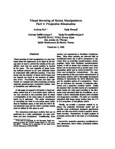
The goal of a machine vision system is to create a model of the real world from images. A machine vision system recovers useful information on a scene from its two-dimensional projections. Since images are two-dimensional projections of the three-dimensional world, this recovery requires the inversion of a many-to-one mapping (see figure 1). R2

P It is assumed that the robot links are joined together with rereplacements R volute joints. Although the equation of motion (1) PSfrag is complex, it has several fundamental properties which can be exploited to facilitate the control system design. For the new control R3 scheme, the following important property is used:

R1

objetivo

l1 Property 1: Considering all revolute joints, the inertial matrix M (q) is lower and upper bounded by [8], [9]: µ1 (q)I ≤ M (q) ≤ µ2 (q)I

q1

(2)

c2

where I stands for the m × n Identity matrix. We should consider that M (q) it is symmetric positive definite inertial matrix.

P


(3)

Fig. 1. Fixed-Camera configuration

218

v q2

c

c3

Property 2: The matrix M˙ (q) − 2C(q, q) ˙ ≡ 0 is skewsymmetric, that is [8], [9], M˙ (q) = C(q, q) ˙ + C(q, q) ˙ T.

l2

c1

u


Let ΣR = {R1 , R2 , R3 } be a Cartesian frame attached to the robot base, where the axes R1 , R2 and R3 represent the robot workspace. A CCD type camera has a ΣC = {C1 , C2 , C3 } Cartesian frame, whose origin is attached at the intersection of the optical axis with respect the geometric center of ΣC . The description of a point in the camera frame is denoted by xC . The position of the camera frame with respect to ΣR is denoted by oC = [oC1 , oC2 , oC3 ]T . The acquired scene is projected on to the CCD. To obtain the coordinates of the image at the CCD plane a perspective transformation is required. We consider that the camera has a perfect aligned optical system and free of optical aberrations, therefore the optical axis intersects at the geometric center of the CCD plane. Finally the image of the scene on the CCD is digitalized, transferred to the computer memory and displayed on the computer screen. We define a new two dimensional computer image coordinate frame ΣD = {u, v}, whose origin is attached to the upper left corner of the computer screen. Therefore the vision system model is given by: · 

u v

·

¸

=



= RT (θ)[xR − ocR ]

x C1  x C2  x C3

λ λ + x C3

αu 0

0 −αv

¸·

x C1 x C2

¸

(7)

where αu > 0, αv > 0 are the scale factors in pixels/m, λ > 0 λ < 0. is the focal length of the camera and λ + x C3 II-C. A new position-based visual servoing scheme for fixedcamera configuration In this section, we present the stability analysis for the position-based visual servoing scheme. The robot task is specified in the image plane in terms of image feature values corresponding to the relative robot and object positions. It is assumed that the target resides in the plane R1 − R2 , depicted in Figure 1. Let [ud vd ]T be the desired image feature vector which is assumed to be constant on the computer image frame ΣD . The desired joints qd are estimated from inverse kinematic in function of [ud vd ]T . The control problem in visual servoing for fixed-camera configuration consists in to designing£a control ¤T law τ in such a reaches the deway that the actual image feature u v £ ¤T sired image feature ud vd of the target. The image fea£ ¤T £ ¤T ˜ v˜ ture error is defined as u = ud − u v d − v , therefore the control aim is to assure that: l´ım t→∞

·

q˜1 q˜2


¸

=

·

qd 1 − q 1 qd 2 − q 2

¸

→0

(8)

The control problem is solvable if a joint motion qd exists such that: αu λ · ¸ ud  λ + xC3 = vd 0 

0 −αv λ λ + x C3



 ·

  T   R(θ)   

xR1 (qd ) xR2 (qd )

−

·

ocR1 ocR2

¸ 

   ¸   (9)

In order to solve the visual servoing control problem, we present the next control scheme with gravity compensation: τ = ∇Ua (Kp , q˜) − fv (Kv , q) ˙ + g(q)

(10)

where q˜ = qd − q ∈ Rn×1 is the error position vector; qd ∈ Rn×1 is the desired position vector; Kp ∧ Kv ∈ Rn×n are the proportional and derivative matrices, respectively; ∇Ua (kp , q˜) represents the artificial potential energy, being a positive definite function, and fv (kv , q) ˙ denotes the damping function, which is a dissipative function, that is, q˙ T fv (kv , q) ˙ > 0. Proposition: Consider the robot dynamic model (1) together with the control law (10), then the closed-loop system is global asymptotically stable, and the visual positioning aim l´ım t→∞ is achieved.

·

q˜1 (t) q˜2 (t)

¸

= 0 ∈ R2

(11)

Proof: The closed-loop system equation obtained by combining the robot dynamic model (1) and control scheme (10) can be written as: d dt

·

q˜ q˙

¸

=

·

−q˙ −1 M (q) [∇Ua (Kp , q˜) − fv (Kv , q) ˙ − C (q, q) ˙ q] ˙ (12)

which is an autonomous differential equation, and the origin of the state space is a equilibrium point. To carry out the stability analysis of equation (12), the following Lyapunov function candidate is proposed:

V (˜ q , q) ˙ =

1 T q˙ M (q) q˙ + Ua (Kp , q˜) , 2

(13)

the first term of V (˜ q , q) ˙ is a positive definite function with respect to q˙ because M (q) is a positive definite matrix. The second one of the Lyapunov function candidate (13), can be interpreted as a potential energy induced by the control law, and is also a positive definite function with respect to the position error q˜, because the term Kp is a positive definite matrix. Therefore, V (˜ q , q) ˙ is both a positive definite and radially unbounded function.

219

¸


The time derivative of the Lyapunov function candidate (13) along the trajectories of the closed-loop equation (12), and after some algebra and considering property 1, can be written as:

To make the stability proof of the equation (16), we proposed the following Lyapunov’s candidate function based in the energy shaping’s methodology [10], [11]:

 p q1 )) pln(cosh(˜  T ln(cosh(˜ q2 )) q˙ M (q)q˙  + V (q, ˙ q˜) = .. 2  . p ln(cosh(˜ qn ))

1 1 T V˙ (˜ q , q) ˙ = q˙T M (q) q¨ − q˙T M˙ (q) q˙ + ∇Ua (Kp , q˜) q˙ 2 2 V˙ (˜ q , q) ˙ = q˙T ∇Ua (Kp , q˜) − q˙T fv (Kv , q) ˙ − C (q, q) ˙ q˙ T +q˙T M˙ (q) q˙ − ∇Ua (Kp , q˜) q˙ V˙ (˜ q , q) ˙ = −q˙T fv (Kv , q) ˙ ≤0

(14)

which is a negative semidefinite function and therefore, it is possible to conclude stability in the equilibrium point. In order to prove local asymptotic stability, the autonomous nature of the closed-loop equation (12) is exploited to apply the LaSalle’s invariance principle [14] in the region Ω:    q˜1     q , q) ˙ =0   q˜2  ∈ R2n : V˙ (˜ q˙ Ω=      q˜ = q˙ = 0 ∈ Rn×1 : V˙ (0, 0) = 0

 p q1 )) pln(cosh(˜  ln(cosh(˜ q2 ))  Kp  ..  . p ln(cosh(˜ qn ))

(15)

The purpose of this section is to exploit the methodology described above with the objective to derive new regulators. We present control scheme with gravity compensation: τ = Kp tanh (˜ q ) − Kv tanh (q) ˙ + g (q)

¸

=

·

(16)

−q˙ M (q)−1 [Kp tanh (˜ q ) − Kv tanh (q) ˙ − C (q, q) ˙ q] ˙

¸

Therefore V (q, ˙ q˜) is a globally positive definite and radially unbounded function. The time derivative of Lyapunov’s candidate function (18) along the trajectories of the closed-loop (17): q˙T M˙ (q)q˙ V˙ (q, ˙ q˜) = q˙T M (q)¨ q+ 2  p q1 )) pln(cosh(˜  ln(cosh(˜ q2 ))  + ..  . p ln(cosh(˜ qn ))

T

" #  tanh q˜  q˜˙  Kp p  ln(cosh(˜ q ))

(19)

and after some algebra and using the property 2 it can be written as:   tanh (q˙1 )  tanh (q˙2 )    V˙ (˜ q , q) ˙ = −q˙T Kv  (20) ≤0 ..   .

which is a negative semidefinite function, therefore we concluded that the equilibrium point is stable. In order to prove the asymptotic stability in a global way, we make use of the autonomous nature of closed-loop (17) when we applied the LaSalle’s invariance principle:

(21)

In the region

(17)

which is an autonomous differential equation, and the origin of the state space is a equilibrium point. Issue 3, Volume 1, 2007

(18)

   

V˙ (q, ˙ q˜) < 0. q˜˙ q¨

.



tanh (q˙n )

Proof: The closed-loop system equation obtained by combining the robot dynamic model (1) and control scheme (15) can be written as:

·

   

The first term of V (q, ˙ q˜) is a positive define function with respect to q˙ because M (q) is a positive definite matrix. The second one of Lyapunov’s candidate function (18) is a positive definite function with respect to error position q˜, because Kp is a positive definite matrix.

since V˙ (˜ q , q) ˙ ≤ 0 ∈ Ω, V (˜ q (t), q(t)) ˙ is a decreasing function of t. V (˜ q , q) ˙ is continuous on the compact set Ω, it is bounded from below on Ω. For example, it satisfies 0 ≤ V (˜ q (t) , q˙ (t)) ≤ V (0, 0). Therefore, the trivial solution is the only solution of the closed-loop system (12) restricted to Ω. Consequently it is concluded that the origin of the state space is locally asymptotically stable. II-D. Examples of application

T

¾ ½· ¸ x ˜ n Ω= ∈ R : V (˜ q , q) ˙ =0 q˙ £ ¤T the unique invariant is q˜T q˙T = 0 ∈ R2n .

220

(22)


III.

E XPERIMENTAL SET- UP

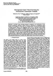
An experimental system for research of robot control algorithms is a direct-drive robot of two degrees of freedom (see Figure 2). The experimental robot consists of two links made of 6061 aluminum actuated by brushless direct-drive servo actuators from Parker Compumotor in order to drive the joints without gear reduction. Advantages of this type of direct-drive actuator includes freedom from backlashes and significantly lower joint friction compared to actuators composed by gear drives.

With reference to our direct-drive robot, only the gravitational torque is required to implement the new control scheme (16), which is available in [8]:

g(q) =

·

38,46 sin (q1 ) + 1,82 sin (q1 + q2 ) 1,82 sin (q1 + q2 )

IV.

¸

[Nm]. (23)

E XPERIMENTAL RESULTS

To support our theoretical developments, this Section presents experimental results of the proposed controllers on a planar robot for the fixed-camera configuration. Desired position Camera

Robot

Computer

PSfrag replacements

Power supply Fig. 3. Fixed-Camera configuration Fig. 2. Direct-drive robot of two degrees of freedom

The motors used in the robot are listed in Table I. The servos are operated in torque mode, so the motors act as a torque source and they accept an analog voltage as a reference of torque signal. Position information is obtained from incremental encoders located on the motors. The standard backwards difference algorithm applied to the joint positions measurements was used to generate the velocity signals.

Three black disks were mounted on the shoulder, elbow and end-effector, respectively. A big black disk for shoulder, a medium black disk on elbow, and a small one for the endeffector.

shoulder disc x

TABLE I S ERVO ACTUATORS OF THE EXPERIMENTAL ROBOT Link Shoulder Elbow

Model DM1050A DM1004C

Torque 50 4

p/rev 1,024,000 1,024,000

PSfrag replacements

q1

elbow disc

q2 The manipulator workspace is a circle with a radius of 0.7 m. Besides position sensors and motor drivers, the robot also includes a motion control board, manufactured by Precision MicroDynamics Inc., which is used to obtain the joint positions. The control algorithm runs on a Pentium host computer. Issue 3, Volume 1, 2007

−y Fig. 4. Disk on robot

221

end-effector disc


The joint coordinates were estimated from predictable centroid replacements using inverse kinematics as is shown in FigurePSfrag 4: q 2 2 l1 = (u2 − u1 ) + (v2 − v1 ) (24) q (u3 − u2 ) + (v3 − v2 )

2

Torque [Nm]

2

l2 =

and

q2 = arc cos

q1 =

³π´ 2

Ã

− arctan

2

2

(u3 − u2 ) + (v3 − v2 ) − l12 − l22 2l1 l2 µ

v2 − v 1 u2 − u 1

¶

− arctan

µ

!

¶ l2 sin (q2 ) l1 + l2 cos (q2 ) (25)

30 25

τ1

20 15 10

5 τ2 0

where l1 , l2 represent the link longitude respectively, u and v are visual information from equation (24) using in figure 4.

0

The centroids of each disc were selected as object feature points. We select in all controllers the desired position in the image plane as [ud ; vd ]T = [198; 107]T [pixels] and the following initial position [u(0); v(0)]T = [50; 210]T [pixels], this q1 (0), q2 (0) = [0; 0]T and q(0) ˙ = 0 [degrees/sec]. The evaluated controllers have been written in C language. The sampling rate was executed at 2.5 ms, while the visual feedback loop was at 33 ms. The CCD camera was placed in front of the robot and its position with respect to the robot R R T frame ΣR was OcR = [0R = [−0,5, −0,6, −1]T c1 , 0 c2 , 0 c3 ] meters, the rotation angle θ = 0 degrees. We use MATLABr version 2007a, applying, the Simulinkr module to carry out the imagine processing. The video signal from the CCDg replacements camera has a resolution of 320x240 pixels in RGB format.

Fig. 6. Torque

50 45 40

Error [degrees]

30

4

5

The figure 5 and 6 shows the experimental results of the controller (16), the proportional and derivative gains were selected as: · ¸ 26,0 0 Kp = 0 1,8 (26) · ¸ 12,0 0 Kv = 0 1,2 and ud = 198 y vd = 107. The transient response with around 3 seconds is fast. The components of the feature position error tend asymptotically close to zero. The experimental results for the controller (16) are shown in figures 5 and 6. The transient response was around 3 seconds. The components of the feature position error tend asymptotically.

τ = Kp arctan (˜ q ) − Kv arctan (q) ˙ + g (q)

25 20 q2

15 10

q1

5 0

2 3 Time [s]

The second one structure used to carry out a position-based visual servoing control is:

35

0

1

1

2 Time [s]

Fig. 5. Error position


3

4

5

(27)

The control structure has a stability proof using Lyapunov theory, the figure 7 and 8 shows the experimental results of the controller structure. The proportional and derivative gains were selected as: · ¸ 17,3 0 Kp = 0 1,2 (28) ¸ · 6,6 0 Kv = 0 1,2

and ud = 198 y vd = 107. The transient response is fast by around 1 second. The components of the feature position error tend asymptotically to a neighborhood close to zero. 222

g replacements INTERNATIONAL JOURNAL OF CIRCUITS, SYSTEMS AND SIGNAL PROCESSING

50

included in the stability analysis. The class of controllers are energy-shaping based, and they are described by control laws composed of the gradient of an artificial potential energy plus a linear velocity feedback. Experimental results with a two degrees of freedom planar robot, using three feature points were presented to illustrate the performance of the control scheme.

45 40

Error [degrees]

35 30 25

R EFERENCES

20

[1] Hutchinson S., G. D. Hager and P. I. Corke, A Tutorial on Visual Servo Control. IEEE Trans. on Robotics and Automation, Vol. 12, No. 5, October 1996, pp. 651-670.

q2

15 10

q1

5 0

[2] Hill J. and W. T. Park, Real Time Control of a Robot with a Mobile Camera. in Proc. 9th ISIR, Washington, D.C., Mar. 1979, pp. 233-246.

0

1

2

3

4

[3] Weiss L. E., A. C. Sanderson, and C. P. Neuman, Dynamic sensorbased control of robots with visual feedback. in IEEE Journal of Robot. Automat., vol. RA-3, pp. 404-417, Oct. 1987.

5

Time [s]

[4] Wilson W. J., C. C. Williams, and Graham S. B. Relative EndEffector Control Using Cartesian Position Based Visual Servoing. IEEE Transactions on Robotics and Automation. vol. 12 No. 5, pp. 684-696. October 1996

Fig. 7. Error position

[5] Kelly R., P. Shirkey and M. W. Spong, Fixed-Camera Visual Servo Control for Planar Robots. IEEE International Conference on Robotics and Automation. Minneapolis, Minnesota, April 1996, pp. 2643-2649.

30

g replacements

[6] Corke P. I. Visual Control of Robot Manipulators A review. Visual Servoing, K. Hashimoto, Ed. Singapore: World Scientific, pp. 1-31, 1993.

25

Torque [Nm]

20

[7] Takegaki M. and S. Arimoto, A New Feedback Method for Dynamic Control of Manipulators. ASME J. Dyn. Syst. Meas. Control, Vol. 103, 1981, pp. 119-125.

τ1

15

[8] Malis E. and S. Benhimane, A Unified Approach to Visual Tracking and Servoing. Robotics and Autonomous Systems, Vol. 52, Issue 1 , 31 July 2005, pp. 39-52.

10

[9] Conticelli F. and B. Allotta, Nonlinear Controllability and Stability Analysis of Adaptive Image-Based Systems. IEEE Trans. on Robotics and Automation, Vol. 17, No. 2, 2001, pp. 208-214.

5 τ2 0

0

1

2 3 Time [s]

4

[10] Park J. and Y.J. Lee, Robust Visual Servoing for Motion Control of the Ball on a Plate. Mechatronics, Vol. 13, Issue 7 , September 2003, pp. 723-738.

5

[11] Malis E. and P. Rives, Robustness of Image-based Visual Servoing with Respect to Depth Distribution Errors. IEEE International Conference on Robotics and Automation. 2003, pp. 1056-1061.

Fig. 8. Torque

The experimental results for the controller (27) are shown in figures 7 and 8. The transient response was around 1 second. The components of the feature position error tend asymptotically. V.

[13] Schramm F., G. Morel, A. Micaelli and A. Lottin, Extended-2D Visual Servoing. IEEE International Conference on Robotics and Automation. 2004, pp. 267-273. [14] Khalil, H. K. (2002). Nonlinear Systems. Prentice–Hall, Upper Saddle River, NJ.

C ONCLUSION

In this paper we have presented a new methodology to design position-based visual servoing for planar robots in fixedcamera configuration. It should be emphasized both that the nonlinear robot dynamics and the vision model have been Issue 3, Volume 1, 2007

[12] Reyes F. and R. Kelly, Experimental Evaluation of Fixed-Camera Direct Visual Controllers on a Direct-Drive Robot. IEEE International Conference on Robotics & Automation. Leuven, Belgium, May 1998, pp. 2327-2332.

[15] Spong M. W. and M. Vidyasagar, Robots Dynamics and Control. John Wiley & Sons, 1989. [16] Chen J., A. Behal, D. Dawson and Y. Fang, 2.5D Visual Servoing with a Fixed Camera. American Control Conference. 2003, pp. 3442-3447.

223