A Voronoi-based Map Algebra Hugo Ledoux and Christopher Gold GIS Research Centre, School of Computing, University of Glamorgan Pontypridd CF37 1DL, Wales, UK
[email protected] —
[email protected]
Abstract Although the map algebra framework is very popular within the GIS community for modelling fields, the fact that it is solely based on raster structures has been severely criticised. Instead of representing fields with a regular tessellation, we propose in this paper using the Voronoi diagram (VD), and argue that it has many advantages over other tessellations. We also present a variant of map algebra where all the operations are performed directly on VDs. Our solution is valid in two and three dimensions, and permits us to circumvent the gridding and resampling processes that must be performed with map algebra.
1 Introduction and Related Work The representation and modelling of geographical data can be done with two contrasting approaches: the object and the field models (Peuquet, 1984; Couclelis, 1992; Goodchild, 1992). The former model considers the space as being ‘empty’ and populated with discrete entities (e.g. a house or a road) embedded in space and having their own properties. The latter model considers the space as being continuous, and every location in space has a certain property (there is something at every location). The property can be considered as an attribute of the location in space, and the spatial variation of an attribute over a certain spatial extent is referred to as a field. This is used to represent continuous phenomena such as the ambient temperature or the humidity of the soil. To store object-based models in a geographical information system (GIS), a variety of data structures with different properties have been developed and implemented. For instance, several GISs explicitly store the adjacency relationships between objects (e.g. TIGER (Boudriault, 1987) and ARC/INFO (Morehouse, 1985)), while some others use non-topological structures
Hugo Ledoux and Christopher Gold (e.g. the so-called spaghetti model) and reconstruct on-the-fly the spatial relationships when needed (Theobald, 2001). By contrast, within the GIS community, field models are more or less synonymous with raster structures (Goodchild, 1992), i.e. a regular tessellation of the plane into squares (pixels) such that each pixel contains the value of the attribute studied. The tools implemented in most GISs to model and analyse different fields are based on the map algebra, which is a framework developed for the analysis of fields stored in a raster format (Tomlin, 1983). With this approach, each field is represented by a grid, and a set of primitive GIS operations on and between fields can be used and combined together to extract information and produce new fields. The framework, and its different operations, are further described in Section 3. Since its conception, several weaknesses and shortcomings of map algebra have been discussed, and many have proposed improvements. Caldwell (2000) introduces a new operator to extend the spatial analysis capabilities, and Eastman et al. (1995) do the same to help the decision-making process. Takeyama (1996) proposes Geo-Algebra, a mathematical formalisation and generalisation of map algebra that integrates the concepts of templates and cellular automata under the same framework. The templates, developed for image algebra (Ritter et al., 1990), extends the concept of neighbourhood of a location, and the addition of cellular automata permits us to model geographic processes. Pullar (2001) also uses the idea of templates and shows how they can help to solve several practical GIS-related problems. As explained in Section 3, the fact that map algebra was developed for raster structures is problematic, firstly because of the dangers of using pixels for analysis (Fisher, 1997), and secondly because complete representations (as in a complete grid) are rarely found in GIS applications, unless datasets come from photogrammetry or remote sensing. Indeed, it is usually impossible to measure geographic phenomena everywhere, and we have to resort to collect samples at some finite locations and reconstruct fields from these samples. Thus, a raster structure implies that some sort of manipulations have already been performed on a field. Kemp (1993) states that “map algebra requires us to enforce a structure on reality rather than allowing reality to suggest a more appropriate structure for our analysis”, and shows that alternative representations (e.g. a triangulated irregular network (TIN), or contour lines; the possible representations are listed in Section 2) are a viable solution. She proposes to have operations— similar to map algebra’s—for modelling fields, which are not all stored under the same representation. She therefore defines a set of rules to convert the different types of fields to other ones when binary operations are applied. For example, if two fields, one stored as a TIN and the other as contour lines, are analysed then the contours must first be converted to TIN before any manipulation is done. Haklay (2004), also to avoid the drawbacks of raster structures, proposes a system where only the data points (samples) and the spatial interpolation function used to reconstruct the field are stored. Each
A Voronoi-based Map Algebra field is thus defined mathematically, which permits us to manipulate different fields in a formulaic form. It should be noticed that the concept of field also generalises to three dimensions, for the modelling of such phenomena as the salinity of water bodies or the percentage of gold in the rock. Mennis et al. (2005) have recently extended map algebra to three dimensions, the tessellation they use is regular (the pixels become cubes called voxels) and the operations are straightforward generalisations of their two-dimensional counterparts. As an alternative to using raster structures and to converting back and forth between different representations of a field, we propose in this paper representing fields with the Voronoi diagram (VD), i.e. a tessellation of space into ‘proximity’ regions. As explained in Section 4, the VD provides a natural way to represent continuous phenomena, and its properties are valid in any dimensions, which makes it ideal for modelling d-dimensional fields. Our proposition is similar to Haklay’s (Haklay, 2004)—get rid of raster and keep only the samples!—but we argue that the VD has many advantages over other tessellations. We also introduce in Section 5 a variant of the map algebra framework where every field and every operation is based on the VD. Perhaps the main contribution of this paper is that the framework is valid in any dimensions. However, since most GIS-related applications are concerned with two and three dimensions, the description and examples will focus on these two cases.
2 Fields A field is a model of the spatial variation of an attribute a over a spatial domain, and it can be represented by a function mapping the location to the value of a, thus a = f (location). (1) The function can theoretically have any number of independent variables (i.e. the spatial domain can have any dimensions), but in the context of geographical data it is usually bivariate (x, y) or trivariate (x, y, z). The domain can also incorporate time as a new dimension, and dynamic fields, such that a = f (location, time), are thus obtained (Kemp, 1993). This notion is useful for modelling phenomena in oceanography or meteorology that continually change over time. Also, notice that in the case of modelling the elevation of a terrain, the function is bivariate as the elevation is assumed to be a property of the surface of the Earth, and no cliffs or overfolds are allowed (as in a so-called 2.5D GIS). Since fields are continuous functions, they must be discretised —broken into finite parts—to be represented in computers. The space covered by a field can be partitioned, or tessellated, into regular or irregular regions. In a regular tessellation, all the regions will be of the same shape and size, while in an
Hugo Ledoux and Christopher Gold irregular one, elements of any shape and size are allowed. In the plane, each region is a polygon, while in three dimensions it is a polyhedron. Regular tessellations arbitrarily divide the space, while irregular tessellations follow the outline of the data points (the samples that were collected to study the field), albeit this is not a requirement. Subdividing the space based on the samples has the main advantage of producing a tessellation that is adaptive to the sample distribution and to the complexity of the phenomenon studied. It also permits us to preserve the samples, which are the only “ground truth” of the field studied, and have even been referred to as the meta-field (Kemp and Vckovski, 1998). Converting scattered samples to a grid means that the original data are ‘lost’. Once the space is tessellated, the field function becomes a piecewise function: to each region is assigned a function describing the spatial variation in its interior. As Goodchild (1992) points out, this function can be constant, linear, or of a higher order. A constant function means that the value of the attribute is constant within one region. An example of the use of a linear function is a TIN: the spatial variation within each region (a triangle) is described by the linear function (a plane) defined by the three vertices (usually samples) lifted to their respective elevation. Akima (1978) shows the advantages of using higher order functions in each region of a TIN—the main one being that the slope of the terrain is continuous everywhere. For the two-dimensional case, some other representations have also been mentioned and used, notably contour lines and irregularly spaced points (the samples to which attributes are attached). In our opinion, the latter representation is incomplete if the spatial function used to reconstruct the field is not explicitly defined, and therefore should not be considered a valid representation of a field. While the dependent variable a in the function representing a field can theoretically be a vector (mostly used in physics to model for instance the magnetic field), we assume in this paper that it is always a scalar. Depending on the scale of measurement used for the values of the attribute, different types of fields are possible: Continuous scale: the value of an attribute can have any value. Temperature, precipitation or salinity are examples because they can be measured precisely. The interval and ratio scales commonly used in GIS, as defined by Stevens (1946), fall into this category. We refer to this type of field as a continuous field. Discrete scale: the values of an attribute are simply labels. Stevens’s nominal and ordinal scales fall into this category. Nominal values are meaningless: an example is a map of Europe where each location contains the name of the country. Ordinal values are labels that can be ordered, e.g. a certain region can be categorised according to its suitability to agriculture from 1 to 5: 1 being poor, and 5 very good. We refer to this type of field as a discrete field.
A Voronoi-based Map Algebra
x f1(x)
f2(x)
fr (x)
(a)
x
x f1
f2
fr
f1(x)
f1
f1(x)
f1
fzones
n(x)
fr (x)
(b)
fr
fr (x)
fr
(c)
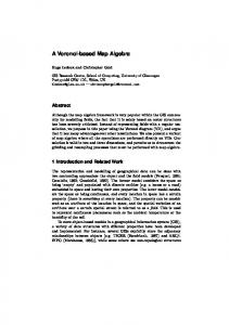
Fig. 1. The map algebra operations with a raster structure. (a) A binary local operation. (b) An unary focal operation. (c) A zonal operation that uses a set of zones (fzones ) stored as a grid.
Notice that here the terms “continuous” and “discrete” refer to the scale of measurement, and not to the spatial continuity of a field. Indeed, both types of fields are spatially continuous, as they are represented by a function. It is also important to notice that not all operations are possible on both types of fields. While many arithmetic operations (addition, subtraction, multiplication, etc.) are possible on continuous fields, they are meaningless for discrete fields.
3 Map Algebra Map algebra refers to the framework, first developed and formalised by Tomlin (1983), to model and manipulate fields stored in a raster structure. It is called an algebra because each field (also called a map) is treated as a variable, and complex operations on fields are formed by a sequence of primitive operations, like in an equation (Berry, 1993). A map algebra operation always takes a field (or many fields) as input and returns a new field as output (the values of the new field are computed location by location). Operations can be unary (input is a single field), binary (two fields) or n-ary (n fields); because n-ary operations can be obtained with a series of binary operations we describe here only the unary and binary cases. Tomlin (1983) describes three categories of operations: Local operation: (Figure 1a) the value of the new field at location x is based on the value(s) of the input field(s) at location x. An unary example is the conversion of a field representing the elevation of a terrain from feet to meters. For the binary case, the operation is based on the overlay in GIS: the two fields f1 and f2 are superimposed, and the result field fr is pointwise constructed. Its value at location x, defined fr (x), is based on
Hugo Ledoux and Christopher Gold both f1 (x) and f2 (x). An example is when the maximum, the average or the sum of the values at each location x is sought. Focal operation: (Figure 1b) the value of the new field at location x is computed as a function of the values in the input field(s) in the neighbourhood of x. As Worboys and Duckham (2004) describe, the neighbourhood function n(x) at location x associates with each x a set of locations that are “near” to x. The function n(x) can be based on distance and/or direction, and in the case of raster it is usually the four or eight adjacent pixels. An unary example is the derivation of a field representing the slope of a terrain, from an elevation field. Zonal operation: (Figure 1c) given a field f1 and a set of zones, a zonal operation creates a new field fr for which every location x summarises or aggregates the values in f1 that are in a given zone. The set of zones is usually also represented as a field, and a zone is a collection of locations that have the same value (e.g. in a grid file, all the adjacent cells having the same attribute). For example, given a field representing the temperature of a given day across Europe and a map of all the countries (each country is a zone), a zonal operation constructs a new field such that each location contains the average temperature for the country. Although the operations are arguably simple, the combination of many makes map algebra a rather powerful tool. It is indeed being used in many commercial GISs, albeit with slight variations in the implementations and the user interfaces (Bruns and Egenhofer, 1997). It should be noticed that the three categories of operations as not restricted to the plane, and are valid in any dimensions (Mennis et al. (2005) have recently implemented them with a voxel structure). Despite its popularity, the biggest handicap to the use of map algebra is arguably that is was developed for regular tessellations only, although the concepts are theoretically valid with any tessellation of space (Takeyama, 1996; Worboys and Duckham, 2004). Using raster structures has many drawbacks. Firstly, the use of pixels as the main element for storing and analysing geographical data has been criticised (Fisher (1997) summarises the issues). The problems most often cited are: (1) the meaning of a grid is unclear (are the values at the centre of each pixel, or at the intersections of grid lines?), (2) the size of a grid (if a fine resolution is wished, then the size of a grid can become huge), (3) the fact that the space is arbitrarily tessellated without taking into consideration the objects embedded in that space. Secondly, in order to perform binary operations, the two grids must “correspond”, i.e. that the spatial extent, the resolution and the orientation of the two grids must be the same, so that when they are overlaid each pixel corresponds to one and only one pixel in the other grid. If the grids do not correspond, then resampling of one grid (or both) is needed. This involves the interpolation of values at regularly distributed locations with different methods such as nearest neighbour or bilinear interpolation, and each resampling degrades the information represented by the grid (Gold and Edwards, 1992). Thirdly, un-
A Voronoi-based Map Algebra less a grid comes from a sensor (remote sensing or photogrammetry), we can assume that it was constructed from a set of samples. Converting samples to grids is dangerous because the original samples, which could be meaningful points such as the summits, valleys or ridges or a terrain, are not present in the resulting grid. Also, when a user only has access to a grid, he often does not know how it was constructed and what interpolation method was used, unless meta-data are available.
4 Voronoi Diagrams Let S be a set of n points in a d-dimensional Euclidean space Rd . The Voronoi cell of a point p ∈ S, defined Vp , is the set of points x ∈ Rd that are closer to p than to any other point in S. The union of the Voronoi cells of all generating points p ∈ S form the Voronoi diagram of S, defined VD(S). In two dimensions, Vp is a convex polygon (see Figure 2a), and in 3D it is a convex polyhedron (see Figure 2b). It is relatively easy to implement algorithms to
p p1 p2 w1
(a)
w2
p3
x w3
w6 w4
p4
p6 w5
p5
(c) (b) Fig. 2. (a) The VD for a set of points in the plane. (b) Two Voronoi cells adjacent to each other in 3D (they share the grey face). (c) The insertion of point x in a VD creates a new Voronoi cell that steals area to its ‘would be’ natural neighbours.
construct a VD in two dimensions (Fortune, 1987; Guibas and Stolfi, 1985) and to delete a single point from one (Devillers, 2002). In three dimensions, the algorithms are more complex but still implementable and efficient. The
Hugo Ledoux and Christopher Gold most popular algorithms to construct a 3D VD are incremental (Edelsbrunner and Shah, 1996; Watson, 1981), which means that a VD is constructed by adding every point one by one. The deletion of a point is also possible in three dimensions, and it is a local operation (Ledoux et al., 2005). All these algorithms exploit the fact that the VD is the dual structure of the Delaunay triangulation—the knowledge of one structure implies the knowledge of the other—and perform their operations on the dual Delaunay triangulation because it is simpler to manipulate triangles/tetrahedra over arbitrary polygons/polyhedra. Since most fields in geography must first be sampled to be studied, we argue in this paper that the Voronoi tessellation has many advantages over other tessellations for representing fields. First, it gives a unique and consistent definition of the spatial relationships between unconnected points (the samples). As every point is mapped in a one-to-one way to a Voronoi cell, the relationships are based on the relations of adjacency between the cells. For example in Figure 2a, the point p has seven neighbours (the lighter grey cells). Note that the points generating these cells are called the natural neighbours of the point p because they are the points that are naturally both close to p and ‘around’ p (Sibson, 1981). This is particularly interesting for Earth sciences because the datasets collected often have highly anisotropic distribution, especially three-dimensional datasets in oceanography or geology because they are respectively gathered from water columns and boreholes (data are therefore usually abundant vertically but sparse horizontally). Second, the size and the shape of Voronoi cells is determined by the distribution of the samples of the phenomenon studied, thus the VD adapts to the distribution of points. Observe in Figure 2a that where the data distribution is dense the cells are smaller. Third, the properties of the VD are valid in any dimensions. Fourth, it is dynamically modifiable, which permits us to reconstruct the field function, and to add or delete samples at will. If a constant function is assigned to each Voronoi cell, the VD permits us to elegantly represent discrete fields. To know the value of a given attribute at a location x, one simply has to find the cell containing x—M¨ ucke et al. (1999) describe an efficient way to achieving that. To reconstruct a continuous field from a set of samples, more elaborate techniques are needed since the VD creates discontinuities at the border of each cell. The process by which the values at unsampled locations are estimated is called interpolation, and many methods have been developed over the years. An interesting one in our case is the natural neighbour interpolation method (Sibson, 1981), because it has been shown by different researchers to have many advantages over other methods when the distribution of samples is highly anisotropic and is an automatic method that does not require user-defined parameters (Gold, 1989; Sambridge et al., 1995; Watson, 1992). This is a method entirely based on the VD for both selecting the samples involved in the interpolation process, and to assign them a weight (an importance). It uses two VDs: one for the set of samples, and another one where a point x is inserted at the interpolation
A Voronoi-based Map Algebra location. The method is based on the area (or volume in three dimensions) that a new point inserted at the interpolation location x ‘steals’ from some of the Voronoi cells already present, as shown in Figure 2c. The resulting function is exact (the samples are honoured), and also smooth and continuous everywhere except at the samples themselves. See Gold (1989) and Watson (1992) for further discussion of the properties of the method, and Ledoux and Gold (2004) for a description of an algorithm to implement it in any dimensions.
5 A Voronoi-based Map Algebra With a Voronoi-based map algebra, each field is represented by the Voronoi diagram of the samples that were collected to study the field. This eliminates the need to first convert to grids all the datasets involved in an operation (and moreover to grids that have the same orientation and resolution), as the VD can be used directly to reconstruct the fields. The permanent storage of fields is also simplified because only the samples need to be stored in a database, and the VD can be computed efficiently on-the-fly and stored in memory (problems with huge raster files, especially in three dimensions, are thus avoided). When a field is represented by the VD, unary operations are simple and robust. To obtain the value of the attribute at location x (for a local operation), the two interpolation methods described in the previous section for discrete and continuous fields can be used directly. Also, the neighbouring function needed for focal operations is simply the natural neighbours of every location x, as defined in the previous section. Figure 3a shows a focal operation performed on a field f1 . Since at location x there are no samples, a data point is temporarily inserted in the VD to extract the natural neighbours of x (the generators of the shaded cells). The result, fr (x), is for example the average of the values of the samples; notice that the value at location x is involved in the process and can be obtained easily with natural neighbour interpolation. Although Kemp (1993) claims that “in order to manipulate two fields simultaneously (as in addition or multiplication), the locations for which there are simple finite numbers representing the value of the field must correspond”, we argue that there is no need for two VDs to correspond in order to perform a binary operation because the value at any locations can be obtained readily with interpolation functions. Moreover, since the VD is rotationally invariant (like a vector map), we are relieved from the burden of resampling datasets to be able to perform operations on them. When performing a binary operation, if the two VDs do not correspond— and in practice they rarely will do!—the trickiest part is to decide where the ‘output’ data points will be located. Let two fields f1 and f2 be involved in one operation, then several options are possible. First, the output data points can be located at the sampled locations of f1 , or f2 , or even both. An example
Hugo Ledoux and Christopher Gold
x
x
f1
n(x)
f1 (x)
f2 (x)
fr (x)
(a)
fr
fr (x)
f1
f2
fr
(b)
Fig. 3. Two Voronoi-based map algebra operations. The top layer represents the spatial extent of the fields, and x is a location for which the value in the resulting field fr (bottom layer) is sought. (a) A unary focal operation performed on the field f1 . The third layer represents the neighbourhood function n(x). (b) A binary local operation performed on the fields f1 and f2 .
where the output data points have the same locations as the samples in f1 is shown in Figure 3b. Since there are no samples at location x in f2 , the value is estimated with natural neighbour interpolation. The result, fr (x), could for example be the average of the two values f1 (x) and f2 (x). It is also possible to randomly generate a ‘normal’ distribution of data points in space (e.g. a Poisson distribution) and to output these. But one should keep in mind that in many applications the samples can be meaningful, and we therefore recommend to always keep the original samples and if needed to densify them by randomly adding some data points. The VD also permits us to vary the distribution of data points across space, for example having more data points where the terrain is rugged, and less for flat areas. As with the other map algebra operations, a zonal operation must also output a field because its result might be used subsequently as the input in another operation. With a Voronoi-based map algebra, the output has to be a VD, and the major difficulty in this case it that we must find a VD that conforms (or approximates) the set of zones. Since zones come from many sources, different cases will arise. The first example is a remote sensing image that was classified into several groups (e.g. land use). Such a dataset can easily be converted to a VD: simply construct the VD of the centre of every pixel. Although this results in a huge VD, it can easily be simplified by deleting all data points whose natural neighbours have the same value. Notice in Figure 4 that the deletion of a single point is a local operation, and the adjacent cells will simply merge and fill up the space taken by the original cell. The second example is with in situ data, for instance in oceanography
A Voronoi-based Map Algebra
x
Fig. 4. Simplification of a discrete field represented with the VD. The data point x is completely surrounded by data points having the same value (here the value is defined by the colour), and deleting it does not change the field.
a dataset indicating the presence (or not) of fish in a water body. The VD of such a dataset can obviously be used directly. The third example is a set of arbitrary zones, such as a vector map of Europe. In two dimensions, it is possible to approximate the zones with a VD (Suzuki and Iri, 1986), but the algorithm is complex and the results are not always satisfactory. A simpler option is to define a set of “fringe” points on each side of a line segment, and label each point with the value associated to the zone. Gold et al. (1996) show that the boundaries can be reconstructed/approximated automatically with Voronoi edges. An example is shown in Figure 5: a set of three zones appears in Figure 5a, and in Figure 5d the Voronoi edges for which the values on the left and right are different are used to approximate the boundaries of the zones. Since each location x in the output field of a zonal operation summarises the values of a field in a given zone, we must make sure that the locations used for the operation are sufficient and distributed all over the zone. Let us go back to the example of the temperature across Europe to find the average in each country. Figure 5a shows a vector map with three countries, and the temperature field f1 is represented by a VD in Figure 5b. Notice that when the two datasets are overlaid (Figure 5c), many Voronoi cells cover more than one zone. Thus, simply using the original samples (with a point-in-polygon operation) will clearly yield inaccurate results. The output field fr , which would contain the average temperature for each country, must be a VD, and it can be created with the fringe method (Figure 5d). Because the value assigned to each data points correspond to the temperature for the whole zone, we suggest estimating, with the natural neighbour interpolation, the value at many randomly distributed locations all over each zone.
6 Discussion The wide popularity of map algebra is probably due to its simplicity: simple operations performed on a simple data structure that is easy to store and manipulate. Unfortunately this simplicity has a hefty price. Tomlin’s map al-
Hugo Ledoux and Christopher Gold
(a)
(b)
(c)
(d)
Fig. 5. (a) A vector map of three zones. (b) A continuous field represented with the VD. (c) When overlaid, notice many Voronoi cells overlap the zones. (d) Approximation of the borders of the zones with the VD.
gebra forces an unnatural discretisation of continuous phenomena and implies a fair amount of preprocessing of datasets, which is usually hidden to the user. As stated in Gold and Edwards (1992), continual reuse and resampling of gridded datasets produce massive degradation of the information conveyed by the data, and can lead to errors and misinterpretations in the analysis. As we have demonstrated in this paper, the tessellation of the space with the Voronoi diagram has many advantages for modelling fields, and a Voronoibased map algebra permits us to circumvent the gridding and resampling processes when we want to manipulate several fields. Although the algorithms to manipulate VDs are admittedly more complex than the ones for raster structures, they are readily available and efficient, and that for the two- and three-dimensional cases.
Acknowledgments We would like to thank the financial support of the EU Marie Curie Chair in GIS at the University of Glamorgan.
A Voronoi-based Map Algebra
References Akima H (1978) A method of bivariate interpolation and smooth surface fitting for irregularly distributed data points. ACM Transactions on Mathematical Software, 4(2):148–159. Berry JK (1993) Cartographic Modeling: The Analytical Capabilities of GIS. In M Goodchild, B Parks, and L Steyaert, editors, Environmental Modeling with GIS, chapter 7, pages 58–74. Oxford University Press, New York. Boudriault G (1987) Topology in the TIGER File. In Proceedings 8th International Symposium on Computer Assisted Cartography. Baltimore, USA. Bruns HT and Egenhofer M (1997) Use Interfaces for Map Algebra. Journal of the Urban and Regional Information Systems Association, 9(1):44–54. Caldwell DR (2000) Extending Map Algebra with Flag Operators. In Proceedings 5th International Conference on GeoComputation. University of Greenwich, UK. Couclelis H (1992) People Manipulate Objects (but Cultivate Fields): Beyond the Raster-Vector Debate in GIS. In A Frank, I Campari, and U Formentini, editors, Theories and Methods of Spatio-Temporal Reasoning in Geographic Space, volume 639 of LNCS, pages 65–77. Springer-Verlag. Devillers O (2002) On Deletion in Delaunay Triangulations. International Journal of Computational Geometry and Applications, 12(3):193–205. Eastman J, Jin W, Kyem A, and Toledano J (1995) Raster procedures for multicriteria/multi-objective decisions. Photogrammetric Engineering & Remote Sensing, 61(5):539–547. Edelsbrunner H and Shah NR (1996) Incremental Topological Flipping Works for Regular Triangulations. Algorithmica, 15:223–241. Fisher PF (1997) The Pixel: A Snare and a Delusion. International Journal of Remote Sensing, 18(3):679–685. Fortune S (1987) A Sweepline algorithm for Voronoi diagrams. Algorithmica, 2:153– 174. Gold CM (1989) Surface Interpolation, spatial adjacency and GIS. In J Raper, editor, Three Dimensional Applications in Geographic Information Systems, chapter 3, pages 21–35. Taylor & Francis. Gold CM and Edwards G (1992) The Voronoi spatial model: two- and threedimensional applications in image analysis. ITC Journal, 1:11–19. Gold CM, Nantel J, and Yang W (1996) Outside-in: An Alternative Approach to Forest Map Digitizing. International Journal of Geographical Information Science, 10(3):291–310. Goodchild MF (1992) Geographical Data Modeling. Computers & Geosciences, 18(4):401–408. Guibas LJ and Stolfi J (1985) Primitives for the Manipulation of General Subdivisions and the Computation of Voronoi Diagrams. ACM Transactions on Graphics, 4:74–123. Haklay M (2004) Map Calculus in GIS: A Proposal and Demonstration. International Journal of Geographical Information Science, 18(2):107–125. Kemp KK (1993) Environmental Modeling with GIS: A Strategy for Dealing with Spatial Continuity. Technical Report 93-3, National Center for Geographic Information and Analysis, University of California, Santa Barbara, USA. Kemp KK and Vckovski A (1998) Towards an ontology of fields. In Proceedings 3rd International Conference on GeoComputation. Bristol, UK.
Hugo Ledoux and Christopher Gold Ledoux H and Gold CM (2004) An Efficient Natural Neighbour Interpolation Algorithm for Geoscientific Modelling. In P Fisher, editor, Developments in Spatial Data Handling—11th International Symposium on Spatial Data Handling, pages 97–108. Springer. Ledoux H, Gold CM, and Baciu G (2005) Flipping to Robustly Delete a Vertex in a Delaunay Tetrahedralization. In Proceedings International Conference on Computational Science and its Applications — ICCSA 2005, LNCS 3480, pages 737–747. Springer-Verlag, Singapore. Mennis J, Viger R, and Tomlin CD (2005) Cubic Map Algebra Functions for SpatioTemporal Analysis. Cartography and Geographic Information Science, 32(1):17– 32. Morehouse S (1985) ARC/INFO: A Geo-Relational Model for Spatial Information. In Proceedings 7th International Symposium on Computer Assisted Cartography. Washington DC, USA. M¨ ucke EP, Saias I, and Zhu B (1999) Fast randomized point location without preprocessing in two- and three-dimensional Delaunay triangulations. Computational Geometry—Theory and Applications, 12:63–83. Peuquet DJ (1984) A Conceptual Framework and Comparison of Spatial Data Models. Cartographica, 21(4):66–113. Pullar D (2001) MapScript: A Map Algebra Programming Language Incorporating Neighborhood Analysis. GeoInformatica, 5(2):145–163. Ritter G, Wilson J, and Davidson J (1990) Image Algebra: An Overview. Computer Vision, Graphics, and Image Processing, 49(3):297–331. Sambridge M, Braun J, and McQueen H (1995) Geophysical parameterization and interpolation of irregular data using natural neighbours. Geophysical Journal International, 122:837–857. Sibson R (1981) A brief description of natural neighbour interpolation. In V Barnett, editor, Interpreting Multivariate Data, pages 21–36. Wiley, New York, USA. Stevens S (1946) On the Theory of Scales and Measurement. Science, 103:677–680. Suzuki A and Iri M (1986) Approximation of a tesselation of the plane by a Voronoi diagram. Journal of the Operations Research Society of Japan, 29:69–96. Takeyama M (1996) Geo-Algebra: A Mathematical Approach to Integrating Spatial Modeling and GIS. Ph.D. thesis, Department of Geography, University of California at Santa Barbara, USA. Theobald DM (2001) Topology revisited: Representing spatial relations. International Journal of Geographical Information Science, 15(8):689–705. Tomlin CD (1983) A Map Algebra. In Proceedings of the 1983 Harvard Computer Graphics Conference, pages 127–150. Cambridge, MA, USA. Watson DF (1981) Computing the n-dimensional Delaunay tessellation with application to Voronoi polytopes. Computer Journal, 24(2):167–172. Watson DF (1992) Contouring: A Guide to the Analysis and Display of Spatial Data. Pergamon Press, Oxford, UK. Worboys MF and Duckham M (2004) GIS: A Computing Perspective. CRC Press, second edition.