Abstract 1. Introduction - Core

Tree-crop interactions and their environmental and economic implications in the presence of carbon-sequestration payments1 Russell Wise and Oscar Cacho Graduate School of Agricultural and Resource Economics, University of New England, Armidale NSW 2351, AUSTRALIA. Contributed Paper to the 47th Annual Conference of the Australian Agricultural and Resource Economics Society, Freemantle, Western Australia, 12-14th February 2003.

Abstract Growing trees with crops has environmental and economic implications. Trees can help prevent land degradation and increase biodiversity while at the same time allow for the continued use of the land to produce agricultural crops. In fact, growing trees alongside crops is known to improve both the productivity and sustainability of the land. However, due to high labour-input requirements, high costs of establishment, and delayed revenue returns, trees are often not economically attractive to landholders. Because of the Kyoto Protocol, and the growing emphasis on market-based solutions to environmental problems, the ability of trees to sequester and store CO2 has altered the economic landscape of agroforestry systems. The economic and management implications of carbon-sequestration payments on agroforestry systems are addressed in this study using a bioeconomic modelling approach. An agroforestry system in Indonesia is simulated using a biophysical process model. A general economic analysis of this system, from the standpoint of individual landholders, is then developed and the implications for management and policy are discussed.

Keywords: agroforestry, bioeconomics, tree/crop interactions, carbon credits, baselines

1. Introduction The Kyoto Protocol (KP) recognizes that land-use activities provide cost-effective opportunities to reduce net greenhouse-gas emissions by acting as carbon sinks and can therefore “contribute to the transition to a lower emissions environment” (Brown et al., 2001; Marland et al., 2001). The KP also allows for emissions trading. The Clean Development Mechanism (CDM), for example, allows Annex I countries to invest in and develop emission-reduction activities such as afforestation and reforestation in non-Annex I countries and to use the reductions against their own commitments2. Examples of activities that sequester and store carbon which could then be traded as Certified Emission Reductions (CERs) are forests and agroforests.

1

This research was funded by the Australian Centre for International Agricultural Research (ACIAR) under project ASEM 1999/093 (http://www.une.edu.au/febl/Econ/carbon/). 2

Annex I lists the 34 countries (developed countries and countries with economies in transition to a market economy) that submitted their first national communications on or before 11 December 1997. Non-Annex 1 countries includes all developing countries not included in this list.

Wise & Cacho, AARES 2003

1

Agroforests are land-use systems where trees, crops and/or livestock are grown in close proximity to each other. Growing trees with crops and livestock or rotating crops with trees have been observed to enhance crop yields, improve soil quality, and recycle nutrients while simultaneously producing subsistence and marketable outputs such as firewood, fodder, fruit and timber. Also, the growing of trees increases the potential to sequester and store carbon, which, in the presence of carbon sequestration payments, adds to the number of marketable outputs being produced. Hence, agroforests are a way of maintaining or enhancing land productivity, sustainability and profitability in the medium to long term. However, when trees and crops grow in close proximity to each other they do not always interact in positive (complementary) ways, they may often interact in negative (competitive) ways too. Complementary interactions between and within crops and trees can occur when pruned tree biomass is added to the system. This leads to microclimatic changes on the soil surface (which affects decomposition rates), weed suppression prior to litter decomposition and increased soil-nutrient levels as the biomass decomposes. Along with the benefits listed above, growing/rotating trees with crops is also known to control erosion and enhance biodiversity (Hairiah et al., 1992). All these benefits, however, are only realized if nutrient outtake is balanced by nutrient input via litter and the strategic use of fertilizers, particularly phosphorous (Sanchez, 1995). Competitive interactions, on the other hand, occur when soil nutrients, water or sunlight are limited and when the growth rates (demand for inputs) of the crop and tree components reach their maximum simultaneously. In the humid tropics, for example, where moisture is not expected to be limiting but fertility may be, trials still show a major competition effect, presumably because of competition for light and nutrients (Sanchez, 1995). Interestingly, most of the successful examples of agroforestry have come from high-potential environments, where water or nutrients were not major limiting factors (Sanchez, 1995). Two types of agroforestry systems are currently practiced in Indonesia and other developing countries. The first, simultaneous agroforestry, is where the tree and crop components grow at the same time and in close enough proximity for interactions to occur (Sanchez, 1995). Examples of this type include alley cropping, contour hedges and homegardens (Nelson et al., 1998; Roshetko et al., 2002). The second, sequential agroforestry, is where the maximum growth rates of the crop and the tree components occur at different times even though both components may have been planted at the same time and are in close proximity (Sanchez, 1995). Examples of this type are shifting cultivation, improved fallows, and some multi-strata systems (Tomich et al., 1998; Grist et al., 1999b; Menz and Grist, 1999; Palm et al., 1999). It is worth noting that the former can be transformed into the latter when, for example, the trees in an alley-cropping system are allowed to grow into a fallow and cropping is discontinued (Sanchez, 1995). In this study we consider only the alley-cropping system. This system involves planting food crops in alleys in-between hedgerows or regularly pruned trees or shrubs. Many factors affect alley-cropping performance: the choice of tree species and crop species, alley width, biomass production, number of crop cycles, time and frequency of pruning, tillage, fertilization and weed dynamics. Alley-cropping systems are successful only in limited and very site-specific circumstances because competition between the different


2

components often exceeds the beneficial, complementary effects. Necessary conditions for alley-cropping systems to succeed include: the soil must be fertile, there must be adequate rains during the cropping season, the land must be prone to erosion, an ample supply of labour coupled with a scarce supply of land must exist, and land tenure must be secure (Sanchez, 1995). This paper presents an economic model of a privately-owned agroforestry system on a smallholding in Indonesia. The agroforest is represented by one tree species (Gliricidia sepium) and one agricultural crop (Maize). The economic model is combined with a biophysical simulation model to analyse the productivity3 and profitability effects of growing trees and crops together in the medium to long term. The effects of carbon sequestration payments on the profitability and management of the system are investigated. The sensitivity of the system to changes in both economic and biophysical variables is then analysed. The paper concludes with implications for policy and management.

2. The economic model This section presents a general economic model of a forest cycle starting with bare ground and including carbon-sequestration payments. The model is based on that developed by Cacho (2001) to estimate the optimal land allocation between forestry and agriculture in a watershed experiencing dryland salinity. The profit function in this paper extends Cacho’s model by including carbon-sequestration payments and carbonmonitoring costs. The profit function faced by a landholder for a given area A over a planning horizon of T years is: T

[

]

V (T , k , x) = [A − k ]∑ yt (k , x) ⋅ p y − c y δ −t t =0 T

+ k ∑ [ht (k , x) ⋅ ph ⋅ ch ]δ −t − c E + VC (T , k , x)

(1)

t =0

V is the profit per hectare obtained by the owner of the agroforestry system using the discount factor δ = 1+r for the discount rate r. The decision variable k is the area planted to trees ( 0 ≤ k ≤ A ) and x is a vector of management variables. The establishment costs are cE. The first term on the right-hand side of (1) is the present value of the cropping area ( A − k ); yt is the annual crop yield, py is the price of the crop and cy is the variable cost of producing the crop. The second term is the present value of the tree harvest; ht is the yield of wood harvested, ph is the price of wood and ch are the variable costs of harvesting the wood. The last term is the present value of carbon-sequestration payments defined as: 3

Measured in terms of tree-biomass accumulation, firewood production and maize yields


3

T

T

t =0

t =0

VC (T , k , x) = k ∑ ∆bt (k , x) ⋅ pC ⋅ δ −t + A∑ [∆st (k , x) ⋅ pC − c M ]δ −t

(2)

where, ∆bt and ∆st are the annual changes in biomass carbon in trees and soil carbon respectively; pC is the price of carbon and cM are annual carbon-monitoring costs. The changes in soil and biomass carbon are dependent upon biophysical processes and management regimes. These dynamics are presented and discussed by Wise and Cacho (2002). Both ∆bt and ∆st can have negative values when more CO2 is released than sequestered. This occurs particularly at final harvest. The optimal area of trees for a given rotation length T, can be determined by maximising equation (1) with respect to k. The economics of forestry and estimation of the optimal forest cycle (the Faustmann model) are well covered in the literature and are not reviewed here. A single cycle is evaluated in this study because this is the relevant measure at the project level, where it cannot be guaranteed that the land will remain in the same use in perpetuity. So this is a financial analysis, rather than a fully-costed economic analysis.

3. Method 3.1 The agroforestry system The system modelled in this study is based on the hedgerow intercopping systems simulated by Sitompul et al. (1992), Nelson et al. (1998), and Magcale-Macandog et al. (1999). In these systems, annual crops are cultivated between contoured hedgerows of perennial shrubs or tree species, usually legumes. Examples of trees typically used as hedgerows in Indonesia are Gmelina, Gliricidia sepium, Leucaena leucocephala, Paraserianthes falcataria and Peltophorum pterocarpa. Gliricidia sepium was chosen for this study because it meets many of the criteria of a successful agroforestry tree species4 and because the WaNuLCAS model (van Noordwijk and Lusiana, 1999) has been parameterized for this species. Desirable features of this species include: it can be grown from cuttings which makes it easy to establish, it is tolerant of acid soil conditions, it grows very quickly, it is nitrogen-fixing and therefore recycles nitrogen through the system and produces mulch with high nutrient values, it also produces several outputs (commercial and subsistence) such as firewood, fencing, mulch and fodder (Hairiah et al., 1992). Annual crops typically cultivated between hedgerows include maize, soybean, mucuna (velvet bean), cassava and rice. These can be grown as multiple-crop rotations such as the maize-soybean-mucuna rotation presented by Sitompul et al. (1992) or as single-crop rotations such as that discussed by Nelson et al. (1998). The crop chosen for this study was maize, as WaNuLCAS is already parameterized for this crop. The model involves simulating the growth of two maize crops per year, between Gliricidia hedgerows, over a

4

See Grist et al. (1999b) and Stewart (1996) for examples of where Gliricidia sepium has been successfully grown as an agroforestry tree species and the reasons why it was successful.


4

25-year rotation. The Gliricidia trees are grown at a planting density of 5,000 trees per hectare and are fully harvested after 25 years. Preparing a hedgerow intercropping system involves removing existing vegetation, usually by burning (Tomich et al., 2002, p. 132), and ploughing the site. Establishing the hedgerows involves constructing bunds (laying out the hedgerows), collecting and planting cuttings, and weeding. Establishing the maize-crop component involves preparing the land between the hedgerows, sowing and fertilizing maize seeds at planting, replanting of maize seeds to replace dead seedlings, and inter-row and hand weeding. These activities need to be done biannually – once each for the wet- and dry-season crops. In practice, maize crops are fertilized using nitrogen, TSP and KCL (Sitompul et al., 1992; Nelson et al., 1998). In this study, however, no fertilizers are applied so the effect of tree residues on land productivity can be determined. To enhance nutrient recycling, pruning is done frequently. Pruning is simulated in WaNuLCAS based on canopy density, where pruning only occurs when the total tree leaf area index (LAI) exceeds a user-defined critical value. Harvesting the pruned material involves removing a predefined percentage of the pruned wood, twigs and leaves from the system. To determine the possible effects that growing trees with crops might have on land productivity, the relative area planted to trees and crops was varied by modelling increasing areas planted to trees relative to crops. For convenience, A was set to 1.0, so 0≤ k≤ 1 and results are expressed per hectare of land-use system (LUS). The area planted to trees was increased at intervals of 0.1 resulting in 11 scenarios. Each of these scenarios was then replicated under three harvest regimes: low (25%), medium (50%) and high (100%). Consequently, 33 scenarios were simulated. The different combinations of tree/crop area and harvest regime are detailed in Table 1. Table 1: Scenarios simulated in WaNuLCAS

Tree Area ( k)

Crop area

(A − k)

Pruning (%)

L

0 0.1 0.2 0.3 0.4 0.5 0.6 0.7 0.8 0.9 1.0

1 0.9 0.8 0.7 0.6 0.5 0.4 0.3 0.2 0.1 0

0 50 50 50 50 50 50 50 50 50 50

25 25 25 25 25 25 25 25 25 25 25

Harvest (%) M H 50 50 50 50 50 50 50 50 50 50 50

100 100 100 100 100 100 100 100 100 100 100

The scenarios listed in Table 1 are referred to by the area (k) planted to trees and an H, M or L indicating whether the harvest regime is 100%, 50% or 25%. For example ‘k = 0.5H’ Wise & Cacho, AARES 2003

5

represents the situation where 50% of the total area is planted to trees and 100% of the pruned material is harvested. The pruning regime and initial soil-carbon level were held constant for all scenarios at 50% and 16.21 Mg C ha-1, respectively. The initial soilcarbon value falls at the lower end of the range of soil-carbon values recorded for soils in Sumatra, Indonesia (Delaney and Roshetko, 1999). In WaNuLCAS, a hedgerow intercopping system is simulated by dividing the total area into four zones and growing the Gliricidia trees in zones 1 and 4 and the maize crops in zones 2 and 3. When the entire area is dedicated to growing maize, zones 1 and 4 are set equal to zero. As the maize area is converted to Gliricidia, zones 1 and 4 are enlarged incrementally and zones 2 and 3 are made smaller by the same magnitude. This is done until the entire area is dedicated to growing Gliricidia i.e. when zones 1 and 4 each comprise 50% of the total area and zones 2 and 3 take up 0% of the area. WaNuLCAS simulates the growth of maize and Gliricidia and generates many outputs. The outputs of most relevance to this study include: harvested tree biomass or firewood (ht), crop yield (yt), standing biomass, standing biomass carbon (SBC) and soil carbon. The annual changes in soil carbon (st), biomass carbon (bt), harvested biomass (ht) and maize-crop yield (yt) obtained from each 25-year simulation were inserted into equations (1) and (2) and net present values were calculated using the base-parameter values presented in Table 2. Table 2. Base parameter values

Parameter ph pC py pS r CL CMt CE Lanp Lanh phw η

Value 45,000 150,000 300,000 2,350 15 6,000 10,000 480,000 1 0.5 80 0.42

Units Rp Mg-1 Rp Mg-1 Rp Mg-1 Rp kg-1 % Rp day-1 Rp ha-1 yr-1 Rp days Mg DM-1 days Mg DM-1 % -

Description firewood price price of carbon price of maize seed price discount rate price of labour annual carbon measuring costs hedgerow establishment costs labour required to prune labour required to harvest % harvest sold as firewood carbon content of wood

Source a e d&f d b&d e g c c c d

Sources: a: CESERF (1999), b: midway between the 10% used by Menz and Magcale-Macandog (1999, p. 10) and the 20% used by Tomich et al. (1998, p. 63), c: adapted from Grist et al. (1999b), d: van Noordwijk and Lusiana (2001), e: Grist et al. (1999a) use $US 5, $US 10 and $US 20 MgC-1, f: Wayan Rusastra et al. (1999, p.152), g: Cacho, Wise and MacDicken (2002)

3.2 Time-averaged carbon stocks and baselines The time-averaged carbon stock for each scenario i of the project ( TACip ) is calculated by summing the annual stock of carbon, Ct, for each scenario i and dividing by the duration of the project (T), for example:


6

T

TACip =

∑C t =1

it

(3)

T

Cit, the annual stock of carbon for scenario i at time t, may represent the biomass carbon (bt), soil carbon (st) or total carbon (bt + st), depending on the quantity of interest. The time-averaged carbon stock provides a simple measure to compare different scenarios in terms of their capacity to sequester carbon, but it does not reflect any differences in the time paths of biomass accumulation. Only carbon over and above that which would have been sequestered without the carbon project is certifiable as an emission reduction and eligible for sale in a carbon market. Therefore, it is necessary to determine a baseline carbon stock with which carbon changes directly attributable to the carbon project may be compared. Two baselines have been identified: a static baseline where it is assumed that the carbon stock of the previous land use remains constant through time, and a dynamic baseline where the carbon stock of the previous land use varies through time. The former may represent an Imperata grassland that contains a stable level of soil carbon and the latter represents a bi-annual maize-cropping system with no fertilizer inputs. The time-averaged total carbon stock of each scenario, relative to each baseline5, is therefore calculated as:

TAC e ij = TAC p i − TAC b j

(4)

where, TAC e ij represents the ‘eligible’ time-averaged total carbon stock for scenario i relative to the previous land-use type (baseline) j; TAC p i is the time-averaged carbon stock of the ‘with-project’ scenario i, and TAC b j represents the time-averaged carbon stock of the previous land-use type (baseline) j. The first term on the right hand side is explained above, and in this case Cit is the annual, total carbon stock (bit + sit). The second term on the right hand side is the time-averaged total carbon stock of the baseline j, and is calculated by summing the annual soil (sjt) and biomass (bjt) carbon stocks for the previous land-use system, j, and dividing by the number of years, T, in the planning horizon: n

TAC

b

ij

=

∑s t =1

jt

+ b jt

T

(5)

The time-averaged soil-carbon stock under Imperata is assumed to be 16.21 Mg C ha-1 and the time-averaged biomass-carbon stock of Imperata grass is taken as 0.7 Mg C ha-1 (Roshetko et al., 2002), hence the total TAC b j for the static baseline is 16.91 Mg C ha-1. 5

Henceforth, the term ‘time-averaged total carbon stocks relative to baseline’ will be referred to as ‘eligible carbon stocks’.


7

The dynamic baseline is calculated as the time-averaged carbon stock of the WaNuLCAS-simulated scenario 1 (tree area, k = 0) and equals 12.32 Mg C ha-1. This scenario only includes the soil-carbon stock. Biomass carbon is not included in this baseline because the maize crops are harvested annually and therefore all the biomass is assumed to be removed annually.

4. Biophysical results This section presents some biophysical results obtained from the WaNuLCAS model. 4.1 Standing biomass carbon

(A) Time-averaged bt

3.5

4.0 3.5

L

3.0

M

(Mg C ha LUS-1)

(Mg C ha of trees-1)

4.5

(B) Time-averaged bt (k/A)

3.0

L

2.5

M H 2.0

H 2.5

1.5 0

0.1 0.2 0.3 0.4 0.5 0.6 0.7 0.8 0.9

1

0

0.1 0.2 0.3 0.4 0.5 0.6 0.7 0.8 0.9

1

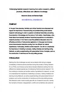
Tree area (k) Tree area (k) Figure 1. The effect of tree area on average standing biomass; (A) carbon per hectare of trees; (B) carbon per hectare of land-use system (LUS), under high (H), medium (M) and low (L) harvest regimes.

For all harvest regimes, average standing biomass carbon (SBC) per hectare of trees (Mg C ha-1) increases as k increases, but only up to k = 0.4 for low and medium harvests and up to k = 0.3 for high harvests (Figure 1A). Further increases in k cause average carbon stocks to decrease. The decrease is caused by increased competition between trees for nutrients and light. This is particularly relevant at high harvests where no nutrients are being returned to the system. The pattern described above, combined with increasing proportions of the farm planted to trees, results in increasing carbon stocks per hectare of land-use system (LUS) up to about k=0.7 (Figure 1B). Beyond k=0.8 there are increases in the carbon stocks both per hectare of trees (Figure 1A) and per hectare of LUS (Figure 1B). This seems to be caused by increased productivity as the lower area of crop decreases competition for nutrients. However, values of k beyond 0.8 may not be desirable by landholders with small plots and who need to produce food for home consumption. So the model results with k > 0.8 do not


8

cause much concern; particularly in view of the economic results presented later, which indicate that the optimal value of k is always below 0.2. 4.2 Soil carbon

Average SC (Mg C ha of trees-1)

Average soil-carbon stock increases dramatically as k increases from 0 to 0.1 ha and then remains relatively constant as k increases further (Figure 2). For high harvests, the soilcarbon stock reaches its highest level when k = 1.0 and involves an increase of 3% compared with the crop-only scenario (k = 0). For medium and low harvests, the soilcarbon stock reaches its highest level at k = 1.0 ha and k = 0.5 ha, respectively. These involve increases in soil carbon of 14% (from 11.85 Mg C ha-1 to 13.79 Mg C ha-1) for medium harvests and 19% (from 11.85 Mg C ha-1 to 14.60 Mg C ha-1) for low harvests. 15

L 14

M 13

12

H

11 0

0.1 0.2 0.3 0.4 0.5 0.6 0.7 0.8 0.9

1

Tree area (k)

Figure 2: Average soil-carbon stock (sit) per hectare of trees, under three harvest regimes.

For low and medium harvest regimes, most of the increase in soil carbon occurs when tree area (k) increases from zero to 0.1. Soil-carbon changes are heavily dependent on the amount of residue inputs available, which is a function of the amount of standing biomass produced. Consequently changes in soil carbon reflect the pattern of SBC production discussed above. Soil-carbon stock, as expected, is inversely related to harvest regime. At high harvests soil-carbon stock is low and it gets progressively larger as harvest regime decreases (Figure 2). 4.3 Harvested tree biomass The output of harvested firewood per hectare of trees planted increases up to a point and decreases thereafter (Figure 3A). For low and medium harvest regimes firewood productivity is not very sensitive to increases in tree area beyond k = 0.2. Maximum harvests of 1.3 Mg C ha-1 and 2.6 Mg C ha-1 are reached at k = 0.2 for low and medium harvests, respectively. At high harvest, firewood output is more sensitive to tree area; a maximum of 5.4 Mg C ha-1 is reached with k = 0.2 (Figure 3A), with a decline to 4 Mg C ha-1 at k=1.0. The decline in firewood production as k increases beyond 0.2 is caused by lower net primary production (NPP) due to increased competition. A lower NPP means less biomass will be available for pruning and harvesting.


9

H

5 4 3

M

2

L

1 0

Firewood (Mg DM ha LUS-1)

Firewood (Mg DM ha trees-1)

6

(A) Harvested firewood per ha of trees

6

(B) Actual harvested firewood per ha of land-use system

5 4

H

3 2

M

1

L

0

0 0.1 0.2 0.3 0.4 0.5 0.6 0.7 0.8 0.9 1

0 0.1 0.2 0.3 0.4 0.5 0.6 0.7 0.8 0.9 1

Tree area (k)

Tree area (k)

Figure 3. The effect of tree area on average harvested biomass under three harvest regimes.

The pattern described above, combined with increasing tree area, results in monotonic but nonlinear increases in actual firewood production per hectare of LUS (Figure 3B). As k increases from 0 to 1.0 the actual amount of firewood harvested increases to 1.07, 2.11 and 3.99 Mg DM for low, medium and high harvests respectively. 4.4 Crop yield

(A) Maize yield per ha of maize 6 M

5

L

4 3 2 1

H

0

Maize-yield (Mg DM ha LUS-1)

Maize-yield (Mg DM ha of maize -1)

When the whole area is planted to maize (k = 0), the average annual maize yield is 4.09 Mg DM ha-1 from two crops per year (Figure 4A). As k is increased from 0 to 0.6, maize yields increase by 29% and 26% under low and medium harvest regimes, respectively, but decline by 86% under high harvest regimes. Most of these changes occur within the first 10 percent of area converted from maize to trees. When k is increased beyond 0.6, maize yields decline under low and medium harvests and remain relatively constant under high harvest, except for an increase as k approaches 1.0. (B) Actual maize yield per ha of landuse system 6 5 4

L

M

3 2 1

H

0

0 0.1 0.2 0.3 0.4 0.5 0.6 0.7 0.8 0.9 1 Tree area (k)

0 0.1 0.2 0.3 0.4 0.5 0.6 0.7 0.8 0.9 1 Tree area (k)

Figure 4. The effect of tree area on maize production


10

Under low and medium harvests, the patterns described above combined with decreasing crop areas as k increases, result in actual maize-yield peaks (per ha of LUS) at k=0.1 (Figure 4B). These results show that under low and medium harvests the benefits from adding pruned biomass to the system outweigh the negative effects of shading and belowground competition for water and nutrients. Whereas the large drop in maize yield under high harvests as k increases is due to the trees out-competing the crops for the very limited resources available with no nutrients returned to the system. The results above are average maize yields over a 25-year period, but they do not reflect temporal changes in yields. The trajectories associated with selected scenarios are presented in Figure 5. Maize yields decline throughout the 25 years for all harvest levels and areas of trees planted. This indicates that two maize crops a year on a continuous basis deplete the nutrients in the soil. The speed of the decline in yields depends on the firewood-harvest regime. The decline is more rapid at high harvests (Figure 5A) and when k is between 0.1 and 0.5. At the low harvest regime, yields decline faster when k = 0 and the decline slows down when trees are planted (Figure 5B). However, the system remains unsustainable under all scenarios used in this study, indicating that more nutrients need to be added to the system to maintain productivity. -1 Maize yield(Mg ha of maize yr-1)

(A) High firewood-harvest regime

(B) Low firewood-harvest regime

12

12

10

10

8

8

k=0

6

6

4

4

2

k=0.5

0

k=0.5

k=0.9

k=0

k=0.9

2

0 10 15 20 25 0 5 10 15 20 25 Time (years) Time (years) Figure 5. The trajectory of maize yield over 25 years for selected values of k and for high (A) and low (B) firewood-harvest regimes. 0

5

5. The baseline As mentioned earlier, only stocks of carbon above the baseline are eligible for trading, so agreement on the baseline is critical for biomass-carbon trading. If the current land use has a fairly stable average carbon content (eg. a pasture), the baseline can be static, represented by a constant stock of carbon overtime. However, if the current land use is


11

unsustainable continuous cropping, as represented in Figure 5, a dynamic baseline is more appropriate; because the ‘business as usual’ consists of decreasing carbon stocks overtime. The trajectories of total carbon stocks (biomass plus soil) are presented for selected scenarios in Figure 6. In the absence of trees (k=0) total carbon decreases overtime. When trees are planted (k>0) total carbon increases during the first few years and decreases thereafter.

Total carbon stock (Mg ha LUS-1)

When trees are planted, higher harvest regimes are associated with quicker declines in total carbon after the peak (compare Figures 6A, 6B and 6C). As with the crop in the previous section, these patterns indicates that this system is unsustainable, but that the relative productivity of the system improves as firewood-harvest regime decreases (more organic matter is returned to the plant-soil system). 21

(A) Low harvest

21

k=0.5

19

(B) Medium harvest

19

17

21 19

k=0.5

17

15 13 11

13

k=0

11

9

15

k=1.0

13

k=0 5

10

15

20

25

k=0

k=1.0

11

9 0

k=0.5

17

15

k=1.0

(C) High harvest

9 0

5

10

15

20

25

0

5

10

15

20

25

Time (years)

Figure 6. The trajectory of total carbon stock, under three firewood-harvest regimes and for selected tree areas (k).

A static baseline could be represented in Figure 6 by a horizontal line at the intercept of all the curves (at 16.2 Mg C ha-1), whereas a dynamic baseline could be represented by the curve labelled k=0. The eligible carbon for any given scenario is obtained by subtracting the baseline carbon from the actual carbon stock. The trajectories of eligible carbon stocks (Figure 7) are the difference between the total carbon stock of three different scenarios and the baseline, based on previous land use. The static baseline represents an Imperata grassland with a constant 16.91 Mg C ha-1. Figure 7A shows that, if landholders were to convert grassland into a maize-Gliricidia system and enter the carbon market, they would be liable for carbon emissions in several years (when eligible carbon stocks are below zero). If the current land use is continuous cropping, the dynamic baseline applies (Figure 7B). Under the dynamic baseline, were landholders to enter a carbon market, they would be eligible for credits on carbon sequestered throughout the rotation for all values of k>0. So the baseline is critical in determining whether landholders will have incentives to adopt agroforestry systems.


12

Eligible carbon (Mg ha -1)

(A) Static baseline 2

(B) Dynamic baseline 8

k=1.0

0

k=1.0

6

-2

k=0.5

4

k=0.5

-4

k=0

-6

2

-8

0 0

5

10

15

Time (years)

20

25

0

5

10

15

20

25

Time (years)

Figure 7. The trajectory of eligible carbon, calculated relative to either a static baseline representing a grassland (A), or a dynamic baseline representing continuous cropping (B) under a medium harvest regime and for selected tree areas (k).

6. Economic analysis The economic performance of any agroforestry system depends on economic variables such as output prices, establishment costs, labour costs and discount rate. Also, for agroforests such as the hedgerow intercropping system simulated in this study, economic performance depends on management decisions such as area planted to crops and trees and the intensity of the harvest regime. Investment in a carbon project will occur only if the net present value (NPV) of the ‘withcarbon’ alternative exceeds that of the ‘without-carbon’ alternative. Three alternatives are considered here: (a) where only traditional outputs (maize and firewood) are accounted for (the ‘no C credits’ alternative); (b) where traditional outputs and carbon are included, and eligible carbon is measured relative to a static baseline; and (c) as in b, but with eligible carbon measured relative to a dynamic baseline. Alternative (a) is implemented by setting the third term in equation (1) equal to zero whereas alternatives (b) and (c) incorporate all three terms in equation (1) but with different baselines as explained in equations (4) and (5). 6.1 Base-case results Economic results under base parameter values are presented in Table 3 for selected scenarios. The financial benefits of growing trees with crops are only realized when the harvest regime is medium or low. Under these regimes (L and M) the maximum NPV is obtained at k=0.1 (Table 3). At high harvest the best alternative is not to grow trees (k=0). The large drops in NPV between k = 0 and k = 0.1, for all scenarios involving high harvest, is due to the decline in


13

crop yields caused by the trees out-competing the crops for soil nutrients and sunlight, with no nutrients being returned to the system, since all prunings are harvested. Table 3. Net Present Values (Rp ’000 ha-1) for selected scenarios Firewood Baseline Harvest

0

0.1

Tree area (k) 0.2 0.3

0.4

0.5

With no C credits

None

L M H

3,473 3,473 3,473

4,316 3,858 -2,342

4,007 3,733 -1,974

3,491 3,251 -1,930

2,991 2,824 -1,702

2,559 2,457 -1,377

With C credits

Static

L M H

3,019 3,019 3,019

4,164 3,626 -2,736

3,927 3,568 -2,303

3,474 3,149 -2,194

3,038 2,785 -1,904

2,670 2,483 -1,513

Dynamic

L M H

3,413 3,413 3,413

4,557 4,019 -2,343

4,320 3,962 -1,910

3,868 3,543 -1,800

3,431 3,178 -1,511

3,064 2,877 -1,120

The low-harvest regime produces higher NPVs under all three baselines (none, static and dynamic) than the medium- and high-harvest regimes. The effect on NPV of carbon trading is very different depending on whether a static or dynamic baseline is used. Under a static baseline it is not worthwhile trading carbon, as this will result in a lower NPV than with no C credits (Rp 4,164,000 vs. Rp 4,316,000). This is because, at tree areas lower than 0.5, there is a net loss of carbon compared with the static baseline and this loss produces a debit in the carbon market. This pattern is reversed when k exceeds 0.5 because the rate of carbon accumulation in the standing biomass now exceeds the rate of soil carbon loss and there is a net gain in carbon compared with the static baseline. When a dynamic baseline is used, it is attractive to trade carbon, as the maximum NPV is higher with than without C credits (Rp 4,557,000 vs Rp 4,316,000). NPVs for all values of k are greater under the dynamic baseline than under the no C credits alternative (Table 3). This is because the dynamic baseline reflects a land-use system that involves carbon losses over 25 years, and the agroforestry system increases the carbon stocks relative to the business-as-usual case. The optimal area to plant to trees with no C credits’ is 0.1 for low and medium harvests and zero for high harvests. The same applies to the two alternatives with C credits. The NPVs are larger when trees are grown at ks between 0.1 and 0.4 compared with the notrees case, even though the direct monetary benefit from the tree component is extremely small. The indirect benefits of growing trees with crops more than compensate for the small direct monetary benefits from forestry over the interval 0