Abstract. State abstraction has been widely used for state aggregation ... senting unknown object quantities in belief states and find- .... schema, solving a generalized planning problem may re- ... to move a transport using the regular state-transforming ac- ..... beling abstract structures with linear inequalities concerning.
Proceedings of the Eighth Symposium on Abstraction, Reformulation, and Approximation (SARA2009)
Abstract Planning with Unknown Object Quantities and Properties Siddharth Srivastava and Neil Immerman and Shlomo Zilberstein Department of Computer Science, University of Massachusetts, Amherst, MA 01003
Abstract
makes their computation infeasible. With such representations, even simple problems like recycling described above will challenge planners, simply because of the size of their solutions. Approaches like conditional non-linear planning (Peot and Smith 1992) address this issue, but are limited in their representation of object quantities and cannot contain the growth in size of the state space due to increasing objects. One approach for dealing with large or unknown numbers of objects is to allow loops over these objects. Such a solution for the recycling problem would be short, with a simple loop of actions, and an included branch for the sensing result with the appropriate action for the current object. Finding such plans presents some difficult challenges: first, finding the loop itself, and second in determining the overall effect, and more importantly, the utility of the loop. We need to be able to distinguish “hard” loops that return to the same world state from desirable loops that make progress. The difficulty is that plans with loops and branches resemble programs and algorithms, for which questions about progress can be undecidable even for single problem instances.
State abstraction has been widely used for state aggregation in approaches to AI search and planning. In this paper we use a powerful abstraction technique from software model checking for representing collections of states with different object quantities and properties. We exploit this method to develop precise abstractions and action operators for use in AI. This enables us to find scalable, algorithm-like plans with branches and loops which can solve problems of unbounded sizes. We describe how this method of abstraction can be effectively used in AI, with compelling results from implementations of two planning algorithms.
Introduction The objective of automated planning is to determine methods for reaching a goal state using domain specific actions. Classical planning concentrates on the most fundamental question in planning by focusing on finding linear sequences of actions that take an input state to a goal state. Conditional planning on the other hand, generalizes this problem in two ways: first, the initial state need not be defined precisely, and second, actions may lead to states with unknown or uncertain properties, which may be clarified using sensing actions. In this paper we focus on the role of abstraction in solving fundamental problems of conditional planning, by assuming that we do not have any probabilistic information about the associated uncertainties. Conditional planning frameworks typically work with sets of possible states, or belief states (Bonet and Geffner 2000; Hoffmann and Brafman 2005). Approaches for conditional planning use a variety of abstraction methods for representing these belief states and computing the effects of actions applied on them. However, existing abstraction mechanisms have a significant shortcoming: they do not provide methods for representing and dealing with unknown quantities of objects. Situations where such representations are required, or would be beneficial, are fairly common. For instance, consider a simplified recycling problem where a recycling robot must pick up objects from a set of unknown number of bins, perform a sensing action to determine recyclability, and store them in appropriate containers. While the core set of actions may be simple, no method for conditional planning can express this problem. Under existing methods, every instance of this problem with k bins forms a distinct state space and needs to be solved separately. This problem is further aggravated by limitations on conditional plan representations: current conditional planners find tree-structured solutions whose exponential size quickly
In this paper, we address the twin problems of representing unknown object quantities in belief states and finding scalable conditional plans by using an abstraction technique based on 3-valued first-order logic which was originally developed for static analysis of programs (Sagiv et al. 2002). This abstraction technique allows us to effectively work with belief states comprised of states with different numbers of objects. Our goal is to be able to find scalable plans with loops and branches along with methods for computing their applicability. We begin by formalizing the desired plan representation and planning framework in the section on Generalized Planning. This leads to a useful observation that makes algorithm-like “generalized” plans more tractable than algorithms for most practical planning domains (Fact 1), including the benchmark planning problems. The algorithmic solution to the recycling problem discussed above is an example of a generalized plan. Such plans do not have to grow with increasing domain size. However, they are difficult to analyze. We mitigate this problem by enriching the abstraction to include more information about the states comprising a belief state. This is described after the description of our state and action representations, in the section on Belief State Representation. We describe how this approach can be used in AI to model belief states with unknown numbers of objects and sensing actions with nondeterministic results. We use this formalization to develop algorithms for generalizing example plans, and for merging these generalizations into plans with complicated loop and branch structures while still being able to determine the class of problems that they solve in a wide range of domains.
c 2009, Association for the Advancement of Artificial Copyright ! Intelligence (www.aaai.org). All rights reserved.
143
Generalized Planning
choose x: C(x)
We take the state-based approach to planning. A domain’s relations, actions, and integrity constraints are used to define a domain schema. Integrity constraints specify characteristics of structures of interest. Action operators map pairs of state and operand instantiations to new states. States are represented using logical structures. Formally, Definition 1 A domain-schema is a tuple !V, A, K" where the vocabulary V = {R1n1 , . . . , Rknk } is a set of predicate symbols together with their arities, A is a set of action operators, and K is a collection of integrity constraints about the domain. Each action operator a(x1 , . . . , xn ) consists of a precondition ϕpre expressed in an appropriate language and a state transition function τa which maps a legal (wrt integrity constraints) state with an instantiation for the operands satisfying the preconditions to another legal state: τa (¯ x) : {(S, i)|S ∈ ST [V]K ∧ (S, i) |= ϕpre } → ST [V]K
h
no
no
su
ch
choose x: D(x) D(x)
setD(x) choose y: E(x,y) B(y)
setR(y)
y
R(x)
setR(x)
no such x
succeed
setD(x) choose y: E(x,y)
R(y) B(y)
R(y)
fail
B(y)
R(y)
setB(y)
Figure 1: Generalized plan for two coloring a graph generalized plan can include meta-actions which update the auxiliary relations. The action of choosing an instantiation of operands is also a simple kind of meta-action. A choice meta-action is specified using the variables to be chosen, and a formula describing the constraints they should meet, e.g. choose x, y : (E(x, y) ∧ ¬R(y)). Solutions to generalized planning problems are called generalized plans. Intuitively, a generalized plan is a full fledged algorithm. Formally, Definition 3 (Generalized plan) A generalized plan Π = !V, E, #, s, T, M" is defined as a tuple where V, E are the vertices and edges of a connected, directed graph; # is a function mapping nodes to actions and edges to conditions; s is the start node and T a set of terminal nodes. The tuple M = !Rm , Am " consists of the vocabulary of auxiliary relations (Rm ) and the set of meta-actions (Am ) used in the plan.
An instance from a domain-schema is a structure in its vocabulary satisfying the integrity constraints. Definition 2 A Generalized planning problem is a tuple !I, D, ϕg " where I is a possibly infinite set of instances, D is the domain-schema, and ϕg is the common goal formula in an appropriate language. I can be represented using a finite representation (e.g., propositional or First-Order formulas).
During an execution, the generalized plan’s run-time configuration is given by a tuple !pc, S, i, R" where pc ∈ V is the current node to be executed; S, the current state on which to execute it; i, an instantiation of the free variables in #(pc), and R, an instantiation over S of the auxiliary relations in Rm . In general, compound node labels consisting of multiple actions and meta-actions can be used for ease of expression. For simplicity, we allow only a single action per node and require that all of an action node’s operands be instantiated before executing that node. Unhandled edges such as those due to an action’s precondition not being satisfied and due to non-exhaustive edge labels are assumed to lead to a default terminal (trap) node. A generalized plan is executed by following edges whose conditions are satisfied, starting with s. After executing the action at a node u, the next possible actions are those at neighbors v of u for which the label of !u, v" is satisfied by (S, i). Non-deterministic plans can be achieved by labeling a node’s outgoing edges with mutually consistent conditions. A generalized plan solves an instance i ∈ I if every possible execution of the plan on i ends with a structure satisfying the goal.
This formulation of the generalized planning problem is expressive enough to capture sophisticated algorithm synthesis problems: Example 1 Consider the graph 2-coloring problem. The vocabulary VG = {E 2 , R1 , B 1 }, consists of the edge relation and the two colors. The set of actions is AG = {colorR(x), colorB(x)}, for assigning the red and blue colors. Their preconditions are respectively ¬B(x), ¬R(x). Integrity constraints stating our graphs are undirected, the uniqueness of color labels, and the coloring condition are given by = ∀x, y
no such x
B(x)
where x ¯ = (x1 , . . . , xn ), ST [V]K is the set of finite structures over V satisfying K, and (S, i) denotes the structure S together with an interpretation for the variables x1 , . . . , xn .
KG
D(x)
y
c su
{∀x(¬(R(x) ∧ B(x))) ∧ (E(x, y) → (E(y, x) ∧ ¬(R(x) ∧ R(y)) ∧¬(B(x) ∧ B(y))))}
We consider the planning problem with IG = ST [VG ]KG , or all structures satisfying the integrity constraints; the domain schema !VG , AG , KG ", and the goal condition ϕ2−color = ∀x(R(x) ∨ B(x)). In addition to the relations from a problem’s domain schema, solving a generalized planning problem may require the use of some auxiliary relations for keeping track of useful information. For example, in a transport domain such relations can be used to store and maintain shortest paths between locations of interest. These paths can then be used to move a transport using the regular state-transforming actions. In order to maintain or extract such information, a
Example 2 A generalized plan for the example discussed above can be found using an auxiliary labeling relation D(x) for nodes whose processing is done. D is initialized to φ and is modified using the meta-action setD(x). The generalized plan is shown in Fig. 1. We use the abbreviation C(x) for B(x) ∨ R(x).
144
We call a generalized planning problem “finitary” if for every instance i ∈ I, the set of reachable states is finite. The simplest way of imposing this constraint is to bound the number of new objects that can be created (or found, in case of partial observability). Finitary domains are practical because they capture most real-world situations and are tractable: Fact 1 In finitary domains, the language consisting of instances that a generalized plan solves is decidable. Finitary domains thus have a solvable halting problem. We could thus conceivably develop efficient algorithms for approximating the preconditions of a generalized plan, and use them to create and extend generalized plans. We measure the quality of a generalized plan as the fraction of solvable problem instances that it solves, or its domain coverage. More specifically, we define Dπ (n) = |Sπ (n)|/|T (n)| where T (n) is the total number of solvable problem instances of size at most n, and Sπ (n) is the number of those that π solves.
C4 C3 C2 C1
L1
Abstraction
dest
Location
Crate
Example 4 The delivery domain with one truck has the following actions: Drive(l), Load(c), Unload(c), SetDrivingDest(l), SenseAndSetDest(c). With loc as the location to drive to, update formulas for Drive(loc) action are: at" (u, v)
:= {at(u, v) ∧ (¬truck(u) ∧ ∀t¬in(u, t))} ∨ {¬at(u, v) ∧ (v = loc ∧ (truck(u) ∨ ∃t(truck(t) ∧ in(u, t))))}
The mechanism of the sensing action SenseAndSetDest() is described in section on Sensing Object Properties. The goal condition is also represented as a formula in FO[TC]. For example, ∀x(crate(x) → delivered(x)). The predicate delivered is updated to True for a crate when the Unload action unloads it at its destination.
Belief State Representation We use an abstraction technique originally developed in TVLA (Three Valued Logic Analyzer), a well-established system for the static analysis of programs (Sagiv et al. 2002). We represent belief states using 3-valued structures (or “abstract structures”), in which each tuple may have a logical value 1 (present in a relation), 0 (not present), or 12 (perhaps present) (Sagiv et al. 2002). This way, an abstract three-valued structure, Sa , represents a possibly infinite set of concrete, two-valued structures denoted as γ(Sa ). Given a domain, we select a set, A, of unary predicates to be the abstraction predicates (all the unary predicates in our examples are abstraction predicates). We define the role that an element of a structure plays as the set of abstraction predicates it satisfies. The idea of the abstraction is that each abstract structure will have at most one element of each role. For example Fig. 2 shows part of a concrete state S1 in the delivery domain, and an abstract structure Sa which encompasses S1 . Sa has two elements, c, #, satisfying the roles, {crate}, {location}, respectively. Both elements of Sa are drawn with double circles indicating that they are summary nodes, i.e. they may represent one or more concrete node. A non-summary node represents a unique concrete node. The edge marked “dest” is drawn as a dotted arrow indicating that the truth value of dest(c, #) is 12 . A truth value of 1 is drawn as a solid line and a truth value of 0 is not drawn. The canonical abstraction of a concrete structure is the least general abstract structure that it represents. (Sagiv et al. 2002). Canonical abstraction is formed with one element for each role that occurs in the concrete structure. This will
The action operator for an action (e.g., a(¯ x)) consists of a set of preconditions and a set of formulas defining the new − value p" of each predicate p. Let ∆+ i (∆i ) be formulas representing the conditions under which the predicate pi (¯ x) will be changed to true (false) by a certain action. The formula for p"i , the new value of pi , is written in terms of the old values of all the relations: (pi (¯ x) ∧ ¬∆− i )
L2
the action; the other holds for arguments on which pi was already true and remains so after the action. These update formulas resemble successor state axioms in situation calculus (Levesque et al. 1998). However, we use query evaluation on possibly abstract structures rather than forward chaining to derive the effect of an action.
Running Example (Delivery) Given a set of crates marked with their destinations at a dock, and a truck in a garage, the goal is to determine each crate’s destination and to deliver it using the truck. All the delivery locations are connected directly with the dock. For simplicity, we assume that each crate represents a unit of cargo equal to the truck’s capacity. As described above, we represent states of a domain by two-valued structures in First-Order logic with transitive closure (FO[TC]). State transitions are carried out using action operators described as a set of formulas in FO[TC], defining new values of every predicate in terms of the old ones. We represent belief states using structures in 3-valued logic (“abstract structures”). The set of initial instances is represented as a finite disjunction of belief states. While the terms “structure” and “state” are interchangeable in our setting, we use the former when dealing with a logic-based mechanism. Example 3 The delivery domain can be modeled using the following vocabulary: V = {crate1 , dock1 , garage1 , location1 , truck1 , delivered1 , in2 , at2 , dest2 }. An example structure, S, for the crate delivery problem discussed above can be described as: the universe, |S| = {c, d, g, l, t}, crateS = {c}, dockS = {d}, garageS = {g}, locationS = {l}, truckS = {t}, deliveredS = ∅, inS = ∅, atS = {(c, d), (t, g)}, destS = {(c, l)}.
∨
L3
Figure 2: Abstraction for representing belief states
State and Action Representation
p"i (¯ x) = (¬pi (¯ x) ∧ ∆+ i )
dest
(1)
The RHS of this equation consists of two conjunctions: one holds for arguments on which pi is changed to true by
145
φ
Role i
S0
fφ
φ Role i
S1
Focus formulas are automatically determined from action update formulas in our approach (Srivastava et al. 2007). Application of an action on an abstract structure thus consists of the following steps: action-specific focus operation, precondition test, an action update for every predicate, and finally, a canonical abstraction resulting in the final structure. This method of action application results in abstract states that encompass all possible real world results.
φ Role i
Role i
S2
Role i
S3
Figure 3: Effect of focus with respect to φ. be a summary element iff there is more than one element of that role in the concrete structure. A relation holds with value 1 in the canonical abstraction if it holds for all tuples represented in the concrete structure and it holds with value 1 2 if it holds for some but not all of the tuples represented. For example, Sa is the canonical abstraction of S1 . In Sa , dest(c, #) holds with value 12 because it holds for (C1, L1), but not (C1, L2). This illustrates the use of the intermediate logical value—to represent a more general set of concrete structures than can be represented in two-valued logic. The truth value 12 can also be used to represent uncertain information about relations in a concrete state. The set of all concrete nodes represented by Sa is denoted γ(Sa ). In Fig. 2, it consists of S1 along with all the other two-valued structures containing one or more crate and one or more location, with the relation dest holding between zero or more pairs of crates and locations. Most of these concrete states are inconsistent for the delivery problem domain. Integrity constraints serve to rule out such structures. For example, constraints stating that every crate must have a unique destination are sufficient to reduce γ(Sa ) to the actually possible real world states. In the rest of this paper, we use γ(Sa ) to refer to the set of concrete states represented by Sa that are consistent with the underlying domain’s integrity constraints. An abstract structure Sa is said to embed Sb iff γ(Sb ) ⊆ γ(Sa ). This can be determined by comparing the truth values for tuples of both structures. The advantage of this methodology is that it allows us to represent and deal with uncertainty in object properties or in numbers of objects. Compact representation of belief states is a key challenge in conditional planning. In this approach, each abstract structure has at most 2a elements where a = |A|, the number of abstraction predicates–even though it can represent an infinite set of similar structures. This limit on structure size also makes abstract state spaces finite.
Dealing with Unknown Quantities In general, objects representing action arguments need to be drawn out from their roles prior to action application on abstract states. The drawing-out operation results in two abstract structures, capturing whether or not the drawn element was the last of its role. This is accomplished using mandatory choice operations which select an action’s operands prior to action application. The range of choices for action operands’ roles can be reduced by providing choice operations with the class of acceptable roles. In the planning approaches described later in this paper, these roles are automatically determined as roles of the chosen concrete elements used in the userprovided example plans. Choice operations mark the element being drawn out with a new abstraction predicate to keep it separated from the existing roles. Truth values of predicates for tuples involving the drawn element are initially the same as those for tuples having the original summary element instead of the drawn element; integrity constraints can make these truth values more precise. We implement this mechanism for dealing with unknown quantities using the focus operation. In Fig. 3 for instance, if integrity constraints restrict φ to be unique and satisfiable, then structure S3 in Fig. 3 would be discarded and the summary elements for which φ() holds in S1 and S2 would be replaced by singletons. These two structures would then represent the cases where we have either exactly one, or more than one object with e’s role. Further, the choice action’s predicate update would set a new predicate (e.g. chosen) to hold for the drawn element for which φ holds. Sensing Object Properties In this paper, nondeterminism arises entirely due to uncertainty about properties of a state. Sensing actions are similar to normal actions, except that their focus formulas represent the property being sensed. In the delivery domain for instance, the sensing action SenseAndSetDest() is applicable on a crate marked with the new (not in the domain’s vocabulary) abstraction predicate chosen, and focuses on the formula ∃x(chosen(x)∧dest(x, y)). An integrity constraint stating that every crate has a unique destination rules out illegal results. Sensing actions can also have predicate updates, to be applied on all possible result structures of the sensing operation: the SenseAndSetDest action sets the targetDest predicate for the chosen crate’s newly focused destination in this way. In general, all the legal possibilities for any predicate with imprecise truth values in an abstract state can be generated using a parameterised sensing action. In this paper however, we work with problems where all the possible sensing actions are specified by the domain.
Action Application on Belief States With the abstraction described above, action update formulas may result in increasingly more imprecise abstract states. This is handled in TVLA using the focus operation with user-specified formulas prior to every action update. The focus operation on a three-valued structure S with respect to a formula ϕ produces a set of structures which have definite truth values for every possible instantiation of variables in ϕ, while collectively representing the same set of concrete structures represented by S. The focus operation wrt a set of formulas works by successive focusing wrt each formula in turn. This process could produce structures that are inherently infeasible. Such structures are either refined or discarded using the integrity constraints. A focus operation with a formula with one free variable on a structure which has only one role (Rolei ) is illustrated in Fig. 3: if φ() evaluates to 12 on a summary element, e, then either all of e satisfies φ, or part of it does and part of it doesn’t, or none of it does.
146
at
Dock
crate dest
Location
at
Dock
crate dest
dest, at at
at
delivered;crate
Garage
Garage
Truck
Truck
S1 chosen;crate Dock
at
Location
Location
dest
at
Dock
dest, at
S2
crate dest
Location dest, at
Choose(crate)
at
at delivered;crate
Garage
delivered;crate
Garage Truck
Truck
S4
S3
Figure 4: A loop in the belief state space of the delivery domain that makes progress in the concrete state space. The dotted edges represent a sequence of actions delivering one crate: Choose(crate), Load(), SenseAndSetDest(), Drive(), UnLoad(), SetDrivingDest(Dock), Drive().
Enriching Canonical Abstraction
Theorem 1 Given a plan with simple loops over an extended-LL domain, and a structure node S in the plan, we can compute a set of linear inequalities whose arguments include initial role-counts and whose solutions are exactly the achievable role-counts at S. These inequalities can be computed in time linear in the number of actions in the plan.
In the preceding sections we demonstrated how abstraction based on 3-valued logic can be used to collapse similar states with different numbers of objects into belief states. Although the focus operation in TVLA provides a method for increasing the precision in these states, in many instances in planning we need greater detail. For instance, Fig. 4 shows the abstract structures obtained while applying some actions in the delivery domain. Abstract structure S1 represents all the infinitely many problem instances with more than one undelivered crates and locations. After applying a sequence of actions (see Fig. 4’s caption) on structure S3 , we may return to the same abstract structure. However, the Choose(crate) operation in this sequence has a branch that doesn’t fall back into the loop and instead results in an abstract state where only one undelivered crate remains. Delivering this crate will lead to the goal. In model checking, where the goal is to find potential failure, finding any such path to a target failure structure is a satisfactory result. In automated planning however, we need more details for such a path of actions to be usable. For instance: • Which concrete member states of the start structure actually reach the goal? • How expensive is the given path to the goal, or, how many iterations of the loop do we need to reach the goal? • What does each iteration of the loop accomplish? Can exit from the loop be guaranteed? Answers to these questions depend on the actual problem instance being worked upon. However, in a large class of problem domains we can compute comprehensive answers that are parametric in terms of the possible problem instances. Note that action application can lead to multiple results (only) because of the focus operation. In order to determine the of class instances solved by a path of actions, we need to find the required condition for each branch at the abstract state where it occurs, and propagate it backwards. Let #R (S # ) denote the number of elements of role R in concrete state, S # . For many planning problems, labeling abstract structures with linear inequalities concerning such role counts provides the information needed to do this. A class of abstraction schemes where this approach works is formalized as extended-LL domains. Further discussion about these domains, proofs, and procedures for finding plan preconditions can be found at (Srivastava et al. 2007). We summarize these results as follows:
Given a generalized plan with simple loops and all the role-counts of a solvable problem instance, these methods can also determine the number of iterations of each loop required to solve the given instance. Action branches in these domains are determined by linear inequalities on role-counts, and the effect of an action on the role-count of a structure is determined by a linear function of its initial role-counts. The effect of a loop on rolecounts also determines if the loop makes progress towards the goal. Discussion The use of summary elements described above provides a method for state aggregation across instances of problems with unknown, or different object quantities. With more information attached to abstract structures, we can effectively apply these methods where conventional stateaggregation has proved useful in AI. As an example, we can conduct a direct search for plans in the abstract state space, simulating a search across infinitely many problem instances. Such a search can also yield powerful loops (the one in Fig. 4 can be found by a search in the delivery domain’s abstract state space). Due to the fixed number of roles, abstract state spaces capturing infinitely many problem instances as described above are finite, and often comparable in size to the corresponding concrete state spaces for moderate problem instances.
A Hybrid Approach for Generalized Planning In this section we use the abstraction and action mechanisms presented above to develop algorithms for generalized planning. We call this system for generalized planning Aranda1 . The overall approach behind these algorithms is to use classical plans to construct a generalized plan. More specifically, we generalize every available example plan using A RANDALearn, and merge it with the existing generalized plan using A RANDA-Merge. The example plans themselves can be generated automatically using classical planners. 1 After an Australian tribe whose number system captures a similar abstraction.
147
Generalizing Example Plans: A RANDA-Learn
Algorithm 1: A RANDA-Merge
The A RANDA-Learn algorithm (Srivastava et al. 2008) uses the abstraction mechanism described above to generalize a given classical plan which solves a single problem instance into a generalized plan with simple loops of actions. The resulting generalized plan typically works for infinitely many problem instances; in extended-LL domains this class can be easily computed. The input to A RANDA-Learn is a pair (π, S0# ), where π = (a1 , . . . , an ) is a solution plan for the concrete structure S0# . The algorithm proceeds as follows: first, π is modified to be applicable to abstract states by replacing its actions’ arguments by their roles, giving us π " . π " is then applied to an abstraction S0 of S0# , keeping only that abstract structure Si at each step which embeds the state Si# obtained by π at that step (this is called “tracing”). Repeated abstract structures in this trace indicate that certain state properties have recurred. With an appropriate abstraction, this means that the same actions can be applied again, and is taken as a cue for recognizing a loop. The loop is formed by merging the two abstract structures in the trace. Note that tracing rejects any structure Si that is not consistent with the result Si# in the concrete example. If these structures are included in the plan as open-ended nodes with no following actions in the final trace, they can be used as a compact representation of situations that were not handled. Small instances of these structures can be used to generate more relevant example plans using classical planners.
Input: Existing plan Π, eg trace tracei Output: Extension of Π if Π = ∅ then Π ← tracei return Π repeat mpΠ , mpt ← findMergePoint(Π, tracei , bpΠ , bpt ) if mpΠ found and not first iteration then attachEdges(Π, tracei , bpt , mpt , mpΠ , bpΠ ) if mpΠ found then bpΠ , bpt ← findBranchPoint(Π, tracei , mpΠ , mpt ) until new bpΠ or mpΠ not found return Π
The overall algorithm works by attaching nodes and edges from the branch point to the merge point (bpt , mpt ) in tracei between bpΠ and mpΠ in Π. If a branch point on Π coincides with the next merge point on Π, Alg. 1 introduces a new loop. The result contains abstract result structures after each step, which can be ignored for extracting the generalized plan. If loops within the resulting generalized plan are simple loops, but with included branches that are caused only by sensing actions, the methods presented in (Srivastava et al. 2007) can be extended to apply to these plans, to find their preconditions and the required number of iterations of each loop. Many kinds of nested loops are allowed under this restriction; we omit a formal classification due to lack of space. Examples of allowed loop structure are illustrated by the plans shown in Fig. 5.
Context-Sensitive Merging: A RANDA-Merge A RANDA-Merge (Alg. 1) uses the representation of possible states (or contexts) as abstract structures by storing abstract structures possible after each action in the generalized plan as determined by A RANDA-Learn. It takes as input an example trace tracei created by A RANDA-Learn, and an existing generalized plan Π. Alg. 1 uses findMergePoint to find the earliest structure in tracei that is embeddable in a structure in Π. In order to provide accurate expressions of loop effects, structures within loops in tracei are not considered during this search in order to reduce the structural complexity of the generated plans; those within loops in Π are allowed. If successful, findMergePoint returns mpΠ and mpt , the nodes on Π and tracei corresponding to these structures. A successful search indicates that the example trace’s actions can be successfully executed starting at mpΠ . However, these actions may not be different from those following mpΠ in Π. In order to minimize the new edges added to Π, after finding merge points, Alg. 1 conducts a search for a branch point using subroutine findBranchPoint. findBranchPoint traverses the edges of tracei and Π starting from the last known merge points mpt and mpΠ , and returns the first pair of subsequent nodes where tracei and Π are not consistent: i.e., either a pair of structures such that none of the successor actions in Π match any of the successor actions in tracei , or, a pair of structures nst , nsΠ such that the structure on Π (#(nsΠ )) does not embed the structure in the trace (#(nst )). This gives us a branch point, where the trace behaved differently from the existing plan.
Implementation and Results In this section we present the results of some of our experiments with prototype implementations of A RANDA-Learn and A RANDA-Merge. The test problems were motivated by benchmarks from the international planning competitions. Incremental results for each problem are shown in Fig. 5. The actual plans are more detailed with choice actions, and include one iteration of the loop learned using the first example prior to the topmost action shown in the figures. Action names were modified in some cases to capture the action arguments. To aid readability, edge labels for results of sensing actions were not drawn. Fire Fighting A room in a building may be on fire. Smoke can be detected from anywhere on a floor iff one of its rooms is on fire. The agent has smoke and heat sensors; it must use the smoke detector and goToNextFloor actions to reach the correct floor, and then use the heat sensors to reach the room with the fire and use the extinguish action to quench the fire. In this problem, the first example plan covered all the floors but found none to be smoky. The second plan started at a smoky floor and proceeded to search for the room with fire. A RANDA-Learn found a loop in this example plan, and Alg. 1 attached the generalization to a structure in the loop obtained using example 1. The last two example plans covered unhandled, boundary conditions where the last floor was smoky or the first room of a floor was on fire. Both the loops of the final plan are simple and make progress by in-
148
senseSmoke−CurFloor()
goToNextBin()
2
mv(T2, L)
go−UnvisitedRoom−CurFloor()
goToNextFloor()
senseType() 2
3
senseHeat−CurRoom()
apply−GlassPreProc(obj)
collect−Glass−Cont(obj) go−UnvisitedRoom−CurFloor()
2
forkLift(kind1, T1)
apply−PaperPreProc(obj)
senseSmoke−CurFloor()
4
mv(T2, D2)
load(kind1, T1)
collect−Paper−Cont(obj)
mv(T1, L) unload(T1)
goToNextBin()
mv(T1,D1)
3
3
senseType()
Fire Fighting
load(kind1,T2)
forkLift(kind1, T2) load(kind1, T2)
4
extinguishFire−CurRoom()
mv(T2, D1)
4
senseHeat−CurRoom()
go−UnvisitedRoom−CurFloor()
load(kind2, T2)
mv(T2,L)
mv(T2,L) 2
apply−GlassPreProc(obj)
forkLift(kind1, T2)
apply−PaperPreProc(obj) mv(T2, D3)
collect−Glass−Cont(obj)
unload(T2)
collect−PaperCont(obj) Recycling
Transport
Figure 5: Segments of computed plans for test problems. Circled numbers indicate components added due to different examples. corresponds to the number of losses, but this number cannot creasing the number of visited floors and rooms. This can be determined using existing methods (Srivastava et al. 2007; be predetermined with the available domain knowledge. 2008). There are no unresolved action branches, indicating Key Observations Results of the proposed approach show that the final structure with “no fire” is always reached. several novel features. In all cases, the generalized Recycling As described in the introduction, a recycling plans cover infinitely many problems of unbounded size. agent must visit different bins, sense the type of material A RANDA-Merge adds only necessary segments from exampresent (paper or glass), apply appropriate pre-processing ple plans. For instance, only edges for the two forkLift operations and collect the material in an appropriate conactions from the entire second example in transport were tainer. The first example plan only encountered paper. The added. Merging action segments into loops is a powerful second plan was created to handle an instance of the situatechnique for increasing the scope of the plan far beyond tion where some bins had glass. The plan handled one bin the individual examples: in the recycling domain, the plan with a glass object and collected it. Alg. 1 created a loop by learned using the first example covers only n of the 2n+1 −1 making the branch point for this example’s trace the same as possible problem instances of size at most n. The second the merge point. This illustrates how even small examples plan on the other hand covers a single specific problem incould be used to identify powerful loops. Example 3 dealt stance. The generalized result using just these two plans with an unhandled branch caused due to the drawing out of covers 2n−1 instances (it assumes that the last two bins have elements from a role (last bin was reached), and example paper). 4 handled the case where the last object was of type glass. We present timing results and domain coverage plots for Computed preconditions match the required number of conthe computed plans for the recycling domain in Fig. 6. For tainers with the number of times the corresponding sensing our plans, this includes the complete time taken to generate branches are taken. the result using the provided examples. We compare these Transport This is a more complicated version of the deresults with the largest plan for recycling (for 7 bins) that livery problem. The roadmap is a Y-shaped graph with dewe could generate using contingent-FF (Hoffmann and Brafpots D1 , D2 , D3 on the end points. Two trucks, T1 and T2 man 2005), a well-established contingent planner. with capacities one and two are originally at D1 and D2 , respectively. The problem is to deliver crates from D1 (of Related Work kind1 ) and D2 (of kind2 ) in pairs with one of each kind Our approach uses abstraction for state aggregation, which to D3 . Location L at the center of the Y can be used to has been extensively studied for efficiently representing unitransfer cargo between the two trucks. There are two nonversal plans using BDD’s (Cimatti et al. 1998), for solving deterministic factors in this problem: crates of kind1 may be MDPs (Hoey et al. 1999; Feng and Hansen 2002), for proheavy, in which case the simple load action drops them and ducing heuristics (Helmert et al. 2007) and for hierarchical a forkLift action must be used; crates left at L may get lost search (Knoblock 1991). Unlike these techniques that only if no truck is present. aggregate states within a single problem instance, we use The first example plan delivered 6 pairs of crates to D3 an abstraction that aggregates states from different problem without experiencing heavy crates or losses. The second exinstances with different numbers of objects. ample found a heavy crate, and delivered it using forkLift An alternative approach for handling the “state explosion” actions instead of load; in the third plan a crate left at L was caused due to increasing numbers of objects is to treat obfound missing when T2 reached L, and another crate had to ject types as resources with quantities (Do and Kambhambe picked up from D1 . The plan computed using these three pati 2003; Hoffmann 2003; Gerevini et al. 2008). Howexamples does not handle one case of a crate of kind1 being ever current approaches to numeric planning only deal with heavy (Fig. 5). This can be detected using the set of unhannumbers as measures of the extent of action effects, such as dled abstract structures and was handled by example plan driving x distance, and cannot work with a unit of these re4. The computed preconditions of the resulting plan include sources as action operands (e.g. load one of the crates into the condition that we must have extra crates of kind1 at D1 the truck, then sense its destination). Further, current apinitially, to compensate for the losses at L. This condition proaches are designed to work with states that include valtells us why extra crates are needed and that their number
149
D(n>
=8) =
Coverage (D)
1
1
CFF-soln7 Gen(Eg 1) Gen(Eg 1+2) Gen(Eg 1..3) Gen(Eg 1..4)
Acknowledgments Support for this work was provided in part by the National Science Foundation under grants IIS-0535061, CCF0541018 and CCF-0830174
0.8 0.6
D(n>
=8) =
0.4
D(n>
=8) =
0.2 0 0
5
References
0.25
Bonet, B., and Geffner, H. 2000. Planning with incomplete information as heuristic search in belief space. In Proc. of AIPS, 52–61. Cimatti, A.; Pistore, M.; Roveri, M.; and Traverso, P. 2003. Weak, strong, and strong cyclic planning via symbolic model checking. Artif. Intell. 147(1-2):35–84. Cimatti, A.; Roveri, M.; and Traverso, P. 1998. Automatic OBDD-based generation of universal plans in non-deterministic domains. In Proc. of AAAI, 875–881. Do, M. B., and Kambhampati, S. 2003. Sapa: A multi-objective metric temporal planner. J. Artif. Intell. Res. 20:155–194. Feng, Z., and Hansen, E. A. 2002. Symbolic heuristic search for factored markov decision processes. In Proc. of AAAI, 455–460. Gerevini, A. E.; Saetti, A.; and Serina, I. 2008. An approach to efficient planning with numerical fluents and multi-criteria plan quality. Artif. Intell. 172(8-9). Hansen, E. A., and Zilberstein, S. 2001. Lao*: A heuristic search algorithm that finds solutions with loops. Artif. Intell. 129(12):35–62. Helmert, M.; Haslum, P.; and Hoffmann, J. 2007. Flexible abstraction heuristics for optimal sequential planning. In Proc. of ICAPS, 176–183. Hoey, J.; St-Aubin, R.; Hu, A.; and Boutilier, C. 1999. SPUDD: Stochastic planning using decision diagrams. In Proc. of UAI, 279–288. Hoffmann, J., and Brafman, R. I. 2005. Contingent planning via heuristic forward search witn implicit belief states. In Proc. of ICAPS, 71–80. Hoffmann, J. 2003. The metric-FF planning system: Translating “ignoring delete lists” to numerical state variables. Journal of Artificial Intelligence Research. Special issue on the 3rd International Planning Competition. Knoblock, C. A. 1991. Search reduction in hierarchical problem solving. In Proc. of AAAI, 686–691. Levesque, H. J.; Pirri, F.; and Reiter, R. 1998. Foundations for the situation calculus. Electronic Transactions on Artificial Intelligence 2:159–178. Levesque, H. J. 2005. Planning with loops. In Proc. of IJCAI, 509–515. Milch, B.; Marthi, B.; Russell, S. J.; Sontag, D.; Ong, D. L.; and Kolobov, A. 2005. BLOG: Probabilistic models with unknown objects. In Proc. of IJCAI, 1352–1359. Peot, M. A., and Smith, D. E. 1992. Conditional nonlinear planning. In Proceedings of the first international conference on Artificial intelligence planning systems, 189–197. Sagiv, M.; Reps, T.; and Wilhelm, R. 2002. Parametric shape analysis via 3-valued logic. ACM Transactions on Programming Languages and Systems 24(3):217–298. Srivastava, S.; Immerman, N.; and Zilberstein, S. 2007. Using Abstraction for Generalized Planning. Technical report, 07-41, Dept. of Computer Science, Univ. of Massachusetts, Amherst. Srivastava, S.; Immerman, N.; and Zilberstein, S. 2008. Learning generalized plans using abstract counting. In Proc. of AAAI, 991– 997. Winner, E., and Veloso, M. 2007. LoopDISTILL: Learning domain-specific planners from example plans. In Workshop on AI Planning and Learning, ICAPS.
280
260 240 220 200 (s) 180 pute m 160 o Num to C 30 140 ber o 120 aken 35 T f Bin e 100 40 Tim s (n)
10
Max
0.5
15
20
25
Figure 6: Domain coverage and time for computation of different solution plans for the recycling problem.
uations for all the numerical variables. (Milch et al. 2005) present a language (B LOG) for defining Bayesian probability models over unknown objects. B LOG models can be considered as abstract representations for possible states, but do not include methods for abstract state transformation needed for action operations in planning. Various approaches have attempted to use loops to make plans and policies more general. Cimatti et al. (2003) consider domains where loops are needed for actions which may have to be repeated for success. Such loops are “hard” loops, in the sense that they return to the exact same problem state. In contrast, our objective is to find loops that make measurable, incremental changes. Hansen and Zilberstein (2001) also present a method for computing policies with hard loops of actions, but in a setting where probabilities of action outcomes and their rewards are used to determine the action which would lead to the best possible value. More recently, Winner and Veloso (2007) presented a method for combining example plans into branching planners with simple loops. However, this approach does not provide techniques for analyzing plan applicability. Levesque (2005) presents an approach (K PLANNER) for iteratively solving problems of increasing sizes and extracting patterns in the solutions to determine simple loops which generalize the example plans. K PLANNER is limited to identifying loops that generalize a single numeric planning parameter.
Conclusions and Future Work In this paper we used an abstraction technique from software model checking for state aggregation and planning in AI. We developed methods to effectively reason about action effects in many problem domains in AI and used them in developing novel algorithms for finding powerful plans that can handle infinitely many problems of unbounded size. To our knowledge, this is the first planning approach capable of dealing with unknown numbers of objects and computing complex loops of operator sequences that make measurable progress towards a desired goal. This approach also provides a novel representation of algorithm synthesis problems in the form of a state-based representation on which AI search techniques can be applied. Directions for future work include general methods for determining progress in more complex plan control structure and development of effective methods for direct plan search.
150