accelerating the hierarchical multi-scale software by spatial clustering ...
Recommend Documents
Apr 2, 2013 - ... Emma J. Cooke2, Zoubin Ghahramani3, Paul D. W. Kirk1¤b, David L. Wild1, ... We have also made available a set of R scripts which can be used to ... Citation: Darkins R, Cooke EJ, Ghahramani Z, Kirk PDW, Wild DL, et al.
Apr 1, 2013 - bioc/html/BHC.html. We have also made available a .... error on the mean. The horizontal dashed line shows the result for the full BHC method.
Specifically concerning geographical data, spatial clustering is a powerful technique that can ...... BERRY, M. J. A.; LINOFF, G. Data mining techniques. ... KHATTREE, R.; NAIK, D. N. Multivariate data reduction and discrimination with SAS.
information from these large and heterogeneous spatial databases. Towards this goal, spatial data mining and knowledge discovery has been gaining ...
RO-400085, Romania ... for restructuring software systems), that identifies the refactorings needed in ... comes an integral part of the software development cy-.
ready to use tool to organize the conceptual domain, to browse and search objects, discover their .... This algorithm is a stochastic optimization technique and it allows to ob- tain, starting from ..... and URLs of a search engine log is introduced.
Thomas Hofmann & Joachim M. Buhmann. Rheinische Friedrich{Wilhelms{Universit at ... paper of Kirkpatrick et al. (Kirkpatrick, Gelatt, &. Supported by the ...
Oct 20, 2011 - is constrained by embedding the graph on an hyperbolic surface of genus g (where the genus is the number ... Topologically embedded graphs on planar surfaces (g = 0) have ...... IEEE Transactions on Neural Networks 16: 645-678. 4. ...
ing algorithms PCM and PCQ, by incorporating the tempo- ral smoothness to ..... [24] to quantitatively compare the clustering performances among all the four ...
Oct 28, 2010 - Cut: Complexity and Experiments ... To achieve a better clustering than agglomerative hierarchical clustering and ..... to B. Thus in total we have.
Mar 12, 2017 - Learning, Sydney, Australia, 2017. .... Each Wk for j < k < J is a convolution along. (u, v0 .... The train and test sets have 50k and 10k colored im-.
exploit the multiscale stochastic structure inherent in SAR imagery. This structure is captured by a set of stochastic models which accurately characterize the evolution in scale .... ing with \2021" and symbol probabilities: p(0)=0.2, p(1)=0.3, and.
KEY WORDS: Cloud Model, Hierarchical Clustering, Data Mining, Weather Classification. ABSTRACT: The paper proposed a method of weather classification based on cloud model and .... Such as CURE, BIRCH, CHAMELEON, etc.
GPUs (e.g., Disk-based Databases & Database Utilities) ... DB2 BLU, SAP Hana, Oracle Dual-format,. Microsoft Columnstore ...... Cloud, mobile, and appliances.
KEY WORDS: Cloud Model, Hierarchical Clustering, Data Mining, Weather ... The paper proposed a method of weather classification based on cloud model and ...
Dendrogram. Specify whether to display the dendrogram. Format. Click the format button to change the plot settings (see Dendrogram Window Options below).
Jan 12, 2015 - means algorithm [6] that is widely used thanks to its convergence speed. It par- titions the data ... arXiv:1501.02560v1 [cs.AI] 12 Jan 2015 .... objects we have to find both nearest objects (xi,xj) to form a cluster. Even- tually, the
similarity between clusters. Suppose we wish to cluster the bivariate data shown in the following scatter plot. In this
Milan Jovovic a, Slavica Jonic a,b, Dejan Popovic a,b,* ... E-mail address: [email protected] (D. Popovic) ...... [9] Pitas I, Milos E, Venetsanopoulos AN.
Feb 10, 2011 - Abstract: Hierarchical clustering has been extensively used in practice, ... Algorithms such as k-means [2], fuzzy c-means [3], divisive and agglomerative hierarchical clustering [4] .... then the whole process is evaluated to find the
Dec 11, 2011 - Clustering Criterion and Agglomerative. Algorithm. Fionn Murtagh (1) and Pierre Legendre (2). (1) Science Foundation Ireland, Wilton Park ...
to organize the data to be clustered in a hierarchical manner, ..... rows and columns indexed by the elements of S. If .... periments described in Section 6.1.
luminosity function of quasars and AGN will be computed with special ... the parallel study of quasar formation and evolution and the History of Star Formation.
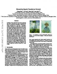
Jan 30, 2018 - Hierarchical Spatial Transformer Network. Chang Shu1,2, Xi Chen2, Qiwei Xie2, Hua Han2,3,4. 1 University of Chinese Academy of Sciences, ...
accelerating the hierarchical multi-scale software by spatial clustering ...
The Hierarchical Multi-Scale (HMS) software, developed at KU Leuven, is a compu- ... which the sum of squared differences within the clusters is minimal.
Accelerating the Hierarchical Multi-Scale (HMS) software by spatial clustering strategies
XIII International Conference on Computational Plasticity. Fundamentals and Applications COMPLAS XIII E. O˜ nate, D.R.J. Owen, D. Peric & M. Chiumenti (Eds)
ACCELERATING THE HIERARCHICAL MULTI-SCALE SOFTWARE BY SPATIAL CLUSTERING STRATEGIES MD KHAIRULLAH∗† , JERZY GAWAD∗ , DIRK ROOSE∗ AND ALBERT VAN BAEL‡ ∗
Department of Computer Science, KU Leuven 3001 Leuven, Belgium e-mail: {md.khairullah, jerzy.gawad, dirk.roose}@cs.kuleuven.be †
Department of Computer Science and Engineering Shahjalal University of Science and Technology, Sylhet-3114, Bangladesh ‡
Department of Materials Engineering, KU Leuven 3001 Leuven, Belgium e-mail: [email protected]
Key words: Multi-scale modeling, Polycrystalline materials, Material properties, Spatial clustering, Approximation error Abstract. In multi-scale simulations of material forming processes, macroscopic zones of nearly homogeneous strain response can be observed. In such zones the evolution of material properties at each finite element integration point can be approximated from the properties at a representative point. We show how these zones can be determined by clustering strategies and utilized to reduce the computational cost of the simulation.
1
INTRODUCTION
The Hierarchical Multi-Scale (HMS) software, developed at KU Leuven, is a computational plasticity tool that takes into account both the strain-driven evolution of the crystallographic texture and the associated plastic anisotropy [1]. The Finite Element (FE) formulation is employed to describe the macroscopic deformation of the material. The homogenized micro-scale stress response is given by appropriate physics-based polycrystalline plasticity models. Anisotropy of the plastic properties is approximated by an analytical plastic potential function. The parameters of this function, together with the texture data form the state variables at the FE integration points. The HMS model assumes that the texture and the coupled plastic properties are initially identical in the whole volume of the material, but may evolve independently in every FE integration point with increasing plastic strain.
932
Md Khairullah, Jerzy Gawad, Dirk Roose and Albert Van Bael
In principle, the texture can change at every time increment of the macroscopic FE model, causing the necessity to compute new parameters of the plastic potential function, resulting in a substantial computational cost. The HMS software partly resolves this issue by reconstructing the function not in every time increment, but only if a given deformation-based criterion is satisfied. Hence, the texture state variable remains constant in each time interval between the updating events. In order to decide whether such an update should take place at an integration point, the recent history of the deformation is being tracked by means of the accumulated plastic strain since the previous updating event. If the updating criterion is satisfied, the accumulated plastic strain tensor is passed to the texture evolution model and a new state is obtained. The accumulated plastic strain at an integration point determines the evolution of the texture and the associated material properties. The plastic slip at an integration point is a function of the plastic strain field during the current and the past time increments during the simulation. We assume that the plastic slip is a scalar representation of the accumulated plastic strain or the deformation history at an integration point. In this paper we present a method to further reduce the simulation time of the HMS model by using spatial clustering of the finite element integration points with respect to the plastic slip field. Clustering is a technique to group data objects, based on information found in the data characterizing the objects and their relationships. The aim is that the objects within a group are similar to one another and different from the objects in other groups. The greater the similarity within a group and the greater the difference between groups, the better. Due to its generic applicability, clustering is used in a broad range of applications, e.g. in materials modeling, material discovery, general finite element simulations and other fields of engineering [2–6]. 2
SPATIAL CLUSTERING IN THE HMS SOFTWARE
Spatial clustering organizes objects into groups, based on distance, connectivity, relative density in space and other feature(s) of interest [7]. The fundamental assumption in this paper is that similar state variables (e.g. crystallographic texture) in neighboring integration points subjected to a similar deformation history (i.e. the plastic strain) would evolve along nearly identical trajectories. It can be expected that the derived macroscopic plastic properties would be similar as well. Therefore, we perform the actual update of the material properties at a single representative integration point per cluster and propagate the updated properties to the other integration points belonging to the cluster. This significantly reduces the number of updates of the material properties and subsequently the overall simulation time. In this work we consistently employ the implementation of the agglomerative clustering algorithm provided by the scikit-learn library for machine learning [8]. This algorithm performs a hierarchical clustering using a bottom up approach. Initially each object is a cluster on its own, and adjacent clusters are successively merged together. A variance-
933
Md Khairullah, Jerzy Gawad, Dirk Roose and Albert Van Bael
minimizing approach is used for the merge strategy. It merges the pair of clusters for which the sum of squared differences within the clusters is minimal. The inputs for the algorithm are the plastic slip values (the feature of interest) at the integration points, the connectivity matrix for the integration points and the number of clusters to find. Within a cluster, we select the integration point with the median of the plastic slip values to be the cluster representative. Note that the clustering algorithm constructs some prescribed number of clusters instead of finding the optimal number of clusters. This limitation remains a fundamental and largely unsolved problem in cluster analysis [9]. Let us consider the specimen in Figure 1a, which is used in the simulation of a tensile test. The boundary conditions are applied as shown in the figure, i.e. the left-hand side is fixed while the deformation is applied towards the right. The figure shows the plastic slip field at the integration points in the final state of the simulation. In Figure 1ab we observe regions of almost homogeneous field values. If one groups the neighboring integration points with similar plastic slip in a cluster, a single update is needed per cluster instead of updates at each integration point, based on the assumption of homogeneity of the underlying texture and the material properties inside the cluster. The corresponding clusters are represented by distinct colors in Figure 1c. For a brief explanation of the proposed strategy, let us consider the two dimensional miniature model in Figure 2 with only 7 elements. Let each element has only one integration point located at the center. Integration points in each element are labeled with A–G. The borders of the clusters are marked by dashed lines, and the cluster representatives are encircled. Notice that although the points C and E show exactly the same field values (the feature of interest), they are put in different clusters since the point D with large difference in the field value is located between them, which violates the connectivity constraint for forming a spatial cluster. In the proposed method only the cluster representatives B, D, E, and G update the material properties. Representative point B propagates its updated properties to A and C, whereas G propagates to F. As D and E are the single member of their own clusters, they only update the material properties but need no propagation. While the underlying micro-structure, texture and the associated material properties are assumed to be the same for the whole cluster, other variables such as the strain and the corresponding stress responses at the integration points are independent of the clusters and evolve individually. 2.1
Static clustering
A static clustering strategy employs a fixed configuration of the clusters, which is constructed based on the field values at a particular moment in the simulation and subsequently kept constant. The advantage of this simple approach is that the overhead related to the construction of the clusters is minimal. However, the choice of the particular moment for constructing the clusters is crucial to obtain a good balance between the number of clusters (and thus the computational cost of the simulation) and the accuracy. We now
934
Md Khairullah, Jerzy Gawad, Dirk Roose and Albert Van Bael
Figure 1: The field of plastic slip in a) the specimen used in the tensile test simulation and b) magnification of the highlighted area. c) Clusters (represented by distinct colors) are constructed according to plastic slip in the highlighted area. consider some specific scenarios. • One can cluster the integration points based on the experience of the user. This naive approach risks to produce a large approximation error. • One can first carry out a FEM simulation under the assumption that the texture and material properties do not evolve. Clustering is then performed based on the field of interest at the final state of the simulation (one could also stop the simulation after a limited number of time increments). This approach is not suited for problems which are strongly influenced by the evolution of texture and material properties. • One can perform a number of time steps in the actual HMS simulation without clustering, and then construct the clusters based on the field of interest. If the clustering is performed in an early time step, it may be that insufficient deformation history is
935
Md Khairullah, Jerzy Gawad, Dirk Roose and Albert Van Bael
Figure 2: Subdivisions of the FE mesh into clusters with respect to the field value (color scale). The elements are labeled with letters, while the cluster representatives are distinguished by circles. available, leading to suboptimal clusters. However, postponing the construction of the clusters leads to less savings in the computational cost. Therefore, we suggest to construct the clusters in the time step in which the update criterion is satisfied for the first time. 2.2
Dynamic adaptive clustering
To overcome the limitations of static clustering, a dynamic adaptive clustering is proposed. In this strategy the integration points are re-assigned to the clusters using criteria based on minimization of the variance w.r.t. the plastic slip among the cluster members. This dynamic approach is more realistic, since it is able to capture the evolution of strain and, more importantly, it does not rely on a single time step to determine the clusters. Hence, compared with static clustering, we expect improvements in the accuracy and, at the same time, performance gains, in particular if relatively large clusters can be retained for a longer time, leading to fewer updates of the material properties. At the beginning of the simulation, the amount of the plastic strain as well as the plastic slip is zero at each integration point and we assign all points to a single cluster. A cluster is split into two clusters if the difference between the maximum and the minimum of the observed field values among the points inside the cluster exceeds a specified threshold value. Of course, this splitting criterion is only tested at the updating events for the texture and material properties. As long as a cluster is not split, the cluster representative prevails the role. At present, for simplicity the adaptation of clustering is based on splitting only and the possibility of merging two clusters is not yet implemented.
936
Md Khairullah, Jerzy Gawad, Dirk Roose and Albert Van Bael
3
ERROR ESTIMATION AND COMPUTATIONAL PERFORMANCE
The spatial approximation of properties over a number of contiguous elements introduces an additional modeling error. To quantify the error, several measures can be analyzed. By using the clustering method, we approximate certain material properties at the non representative members in a cluster by the properties at the cluster representative. More specifically, the plastic anisotropy model is utilized uniformly inside the cluster. The coefficients of the anisotropy model are periodically re-identified to follow the evolution of anisotropy solely at the cluster representative. This approximation also affects the field values that are calculated based on the plastic properties. Hence, we attempt to estimate the approximation error in both the material properties and the affected field values. 3.1
Approximation error in terms of material properties
Let us consider the q-value, which characterizes the plastic anisotropy under uniaxial tensile loading. The q-value is defined as r q= , (1) 1+r where r is the Lankford coefficient. The q-value can be readily derived from the plastic potential function available at each integration point. Provided that the loading conditions in a considered process approximate uniaxial loading along a given direction, the q-value calculated in this direction provides accurate characterization of material behavior. Bearing in mind that the evolution of anisotropy also affects the other loading directions, we calculate the q-value in the range of 0◦ to 180◦ w.r.t. rolling direction with angular resolution of 1◦ . As a consequence, the q-value at a point i is given by a vector of length 181, denoted here by qi . To compare the mismatch at a point we calculate the Euclidean distance of the q-values at a point computed with the original HMS software that does not exploit spatial clustering and the q-values at the representative point computed with the improved HMS software, which is extended with the spatial clustering feature. Note that the original HMS is equivalent to the improved HMS using the finest clusters, i.e. one integration point per cluster. The relative approximation error for the plastic anisotropy or the q-value at a point i is given by qi − q cr(i) q ei = × 100%, (2) qi where cr(i) is the representative point of the cluster to which point i belongs, q and q are the anisotropy values with the original HMS and the improved HMS, respectively. To estimate the approximation error for the whole model we calculate the average value n
e¯q =
1 q e, n i=1 i
937
(3)
Md Khairullah, Jerzy Gawad, Dirk Roose and Albert Van Bael
with n the number of integration points. 3.2
Approximation error in terms of field values
The plastic strain during a time step is affected by the approximation of the material properties using the clustering strategy. As the plastic slip field in the final state of the simulation contains the total plastic deformation history, it also summarizes the total affect of the approximation and is selected for comparison with the original HMS. Unlike the q-value, this scalar value is directly computed at each integration point. Hence, we compute the relative approximation error in the plastic slip field at point i as eγi =
|γi − γi | × 100%, γi
(4)
where γ and γ are the plastic slip values with the original HMS and the improved HMS respectively. Like the previous case, we also compute the average of the error for the whole model n 1 γ e¯γ = e . (5) n i=1 i 3.3
Performance metrics
We measure the relative performance improvement in terms of the calculation time by the speedup sc , defined as tr sc = , (6) tc where tr is the simulation time with the original HMS software and tc is the simulation time with the improved HMS. By using the methods proposed above, we only speed up the part of the software responsible for the evolution of texture and the associated material properties. If that part represents a fraction f of the execution time, then the speedup is limited by smax =
1 . 1−f
(7)
Hence, if f =96%, as in the simulations performed below, smax =25. The expected speedup is 1 se = ≤ smax , (8) (1 − f ) + nnc f with nc the number of clusters used in the improved HMS software, cf. Amdahl’s law [10].
4
RESULTS AND DISCUSSIONS
Tensile test simulations with the improved HMS software were run for the specimen presented in Figure 1 with the setup described in section 2. We compare the accuracy and
938
Md Khairullah, Jerzy Gawad, Dirk Roose and Albert Van Bael
the computational gain by the improved HMS with the original HMS. In all simulations the texture and material properties at an integration point are updated if the norm of the accumulated plastic strain exceeds 0.05. 4.1
Static clustering
As described in section 2.1, the clusters are formed at the first event of texture and material properties update to obtain a balance between savings in computational cost and accuracy of the simulation. One may assume that a clustering based on the field values in the final state of the simulation would lead to a more accurate simulation. Although not practical (because of the computational cost), we have also performed simulations with static clustering based on the fields values in the final state of the simulation, for comparison purposes. Figure 3 shows the measured approximation error for the plastic anisotropy (q-value), given by (3), for varying number of clusters. Figure 4 presents a comparison between the approximation error in the affected plastic slip field, given by (5), and the corresponding speedup, given by (6). Although the accuracy in the plastic anisotropy (q-value) is high (less than 0.5%) and quite similar for both clusterings, clustering based on the field values in the final state of the simulation leads to a remarkably lower error for the plastic slip especially for a low number of clusters. The number of clusters for which a high speedup and an acceptable accuracy is achieved is indicated by the dotted vertical line. clustering at the first update
clustering at the final state
% error in anisotropy (q-value)
0.6 0.5 0.4 0.3 0.2 0.1 0 1
10
100
1000
10000
# clusters
Figure 3: Approximation error in plastic anisotropy (q-value) for varying number of clusters out of 2226 integration points in the model. We measured that the evolution of texture and the associated material properties consumes 96% of the simulation time. Figure 5 compares the speedup obtained by the improved HMS software with the expected speedup for a varying number of clusters, see (8). The actual speedup is lower than the expected speedup due to some overhead.
939
Md Khairullah, Jerzy Gawad, Dirk Roose and Albert Van Bael
error (clustering at the first update) speedup
error (clustering at the final state) 30
9
25
7
20
6 5
15
4
10
3 2
speedup
% error in plastic slip
8
5
1
0 10000
0 1
10
100
1000
# clusters
Figure 4: Approximation error in plastic slip and speedup for varying number of clusters. expected speedup
actual speedup
30 25
speedup
20 15 10 5 0 1
10
100
1000
10000
# clusters
Figure 5: Actual speedup compared to the expected speedup for varying number of clusters. 4.2
Adaptive clustering
A set of different tensile test simulations with the same specimen were run using adaptive clustering. We mentioned earlier that a cluster is split if the difference between the maximum and the minimum of the plastic slip among the cluster members exceeds the specified threshold value. If this threshold value increases, the chance of splitting a cluster decreases. Subsequently fewer clusters are constructed and the required number of update operations is reduced and a larger speedup is achieved. In Figure 6 we observe that the approximation error in final q-value decreases with decreasing threshold values. Figure 7 represents the effect of the adaptive clustering approach in the speedup and the approximation error in the affected field for varying threshold value for splitting. Again,
940
Md Khairullah, Jerzy Gawad, Dirk Roose and Albert Van Bael
the dotted vertical line indicates the threshold value for which a high speedup is obtained while maintaining an acceptable approximation error. average of the error in anisotropy (q-value)
% error in anisotropy (q-value)
0.6 0.5 0.4 0.3 0.2 0.1 0 2
0.2
0.02
threshold value on plastic slip for splitting a cluster
Figure 6: Approximation error in plastic anisotropy for varying threshold value for splitting a cluster.
error
speedup
9
35
8
30 25
6 5
20
4
15
3
speedup
% error in plastic slip
7
10
2 5
1 0 2
0.2
0 0.02
threshold value on plastic slip for splitting a cluster
Figure 7: Approximation error in plastic slip and speedup for varying threshold value for splitting a cluster. Figure 8 compares the clustering approaches w.r.t. obtained speedup and accuracy. We observe that dynamic clustering is superior to static clustering (based on the field values at the first updating event) in terms of accuracy. However, clustering based on the field values in the final state of the simulation produces the least error, but is not practical because of the computational cost. The accuracy of the dynamic approach is closer to this
941
Md Khairullah, Jerzy Gawad, Dirk Roose and Albert Van Bael
best case scenario, especially for higher speedup. Thus, we can infer that the dynamic adaptive approach can better capture the real dynamics and the deformation history. clustering at the first update dynamic clustering
clustering at the final state
5 4.5 % error in plastic slip
4 3.5 3 2.5 2 1.5 1 0.5 0 20
18
16
14
12
10
8
6
4
2
speedup
Figure 8: Approximation error by the proposed methods for varying speedup.
5
CONCLUSIONS AND FUTURE WORK
The presented results show that spatial clustering can considerably reduce the computational cost of the HMS model while retaining acceptable accuracy. Generally, dynamic clustering is preferable to static clustering. The approximation error and the computational benefit depend on the number of clusters used. A certain trade-off has to be made: by increasing the number of clusters, the approximation error can be decreased, but at the same time the computational cost increases. At present we only consider the plastic slip value at an integration point as the feature of interest for clustering. As described earlier, this field is a scalar representation of the plastic strain tensorial field, whereas the strain modes also influence the evolution of the texture and the associated material properties. We intend to implement a strain mode aware clustering and updating. In the current approach of adaptive clustering, only splitting of clusters is considered. We can also consider merging two adjacent clusters, which will effectively reduce the number of active clusters and update operations. ACKNOWLEDGMENTS The authors gratefully acknowledge the financial support from the Knowledge Platform M2Form, funded by IOF KU Leuven, and from the Belgian Federal Science Policy agency, contracts IAP7/19 and IAP7/21. The computational resources and services used in this work were provided by the VSC (Flemish Supercomputer Center), funded by the Hercules Foundation and the Flemish Government department EWI.
942
Md Khairullah, Jerzy Gawad, Dirk Roose and Albert Van Bael
REFERENCES [1] Gawad, J., Van Bael, A., Eyckens, P., Samaey, G., Van Houtte, P. and Roose, D. Hierarchical multi-scale modeling of texture induced plastic anisotropy in sheet forming. Computational Material Science (2013) 66:65–83. [2] Duartea, C.A., Liszka, T.J. and Tworzydlob, W.W. Clustered generalized finite element methods for mesh unrefinement, non-matching and invalid meshes. International Journal for Numerical Methods in Engineering (2006):1–28. [3] Bras, R.L., Damoulas, T., Gregoire, J.M., Sabharwal, A., Gomes, C.P. and Dover, R.B.V. Computational thinking for material discovery: bridging constraint reasoning and learning. CROCS 2010 - 2nd International Workshop on Constraint Reasoning and Optimization for Computational Sustainability (2010). [4] Varde, A.S., Rundensteiner, E.A., Ruiz, C., Brown, D.C., Maniruzzaman, M. and Sisson Jr., R.D. Integrating clustering and classification for estimating process variables in materials science. In the Proceedings of the Twenty-First National Conference on Artificial Intelligence and the Eighteenth Innovative Applications of Artificial Intelligence Conference (2006) 13:495–496 (Preface). [5] Nakano, A. Fuzzy clustering approach to hierarchical molecular dynamics simulation of multiscale materials phenomena. Computer Physics Communications (1997) 105(2–3):139–150. [6] Ferreira, P.G., Silva, C.G., Azevedo, P.J. and Brito, R.M.M. Spatial clustering of molecular dynamics trajectories in protein unfolding simulations. Computational Intelligence Methods for Bioinformatics and Biostatistics, Lecture Notes in Computer Science (2009) 5488:156–166. [7] Han, J., Kamber, M. and Tung, A.K.H. Spatial clustering methods in data mining: a survey. Geographic Data Mining and Knowledge Discovery, Research Monographs in GIS (2001) [8] Pedregosa, F., Varoquaux, G., Gramfort, A., Michel, V., Thirion, B., Grisel, O., Blondel, M., Prettenhofer, P., Weiss, R., Dubourg, V., Vanderplas, J., Passos, A., Cournapeau, D., Brucher, M., Perrot, M. and Duchesnay, E. Scikit-learn: machine learning in Python. Journal of Machine Learning Research (2011) 12:2825–2830. [9] Hardy, A. On the number of clusters. Computational Statistics and Data Analysis (1996) 23:83–96. [10] Amdahl, G.M. Validity of the single-processor approach to achieving large scale computing capabilities. In AFIPS Conference Proceedings (1967) 30:483–485.