Remote Sens. 2015, 7, 12654-12679; doi:10.3390/rs71012654 OPEN ACCESS
remote sensing ISSN 2072-4292 www.mdpi.com/journal/remotesensing Article
Accuracy Optimization for High Resolution Object-Based Change Detection: An Example Mapping Regional Urbanization with 1-m Aerial Imagery Kenneth B. Pierce Jr. WA Department of Fish and Wildlife, Habitat Science Division, 1111 Washington St SE, Olympia, WA 98501, USA; E-Mail:
[email protected]; Tel.: +1-360-902-2564; Fax: +1-360-902-2946 Academic Editors: Soe Myint and Prasad S. Thenkabail Received: 14 May 2015 / Accepted: 18 September 2015 / Published: 25 September 2015
Abstract: The utility of land-cover change data is often derived from the intersection with other information, such as riparian buffers zones or other areas of conservation concern. In order to avoid error propagation, we wanted to optimize our change maps to have very low error rates. Our accuracy optimization methods doubled the number of total change locations mapped, and also increased the area of development related mapped change by 93%. The ratio of mapped to estimated change was increased from 76.3% to 86.6%. To achieve this, we used object-based change detection to assign a probability of change for each landscape unit derived from two dates of 1 m US National Agriculture Imagery Program data. We developed a rapid assessment tool to reduce analyst review time such that thousands of locations can be reviewed per day. We reviewed all change locations with probabilities above a series of thresholds to assess commission errors and the relative cost of decreasing acceptance thresholds. The resultant change maps had only change locations verified to be changed, thus eliminating commission error. This tool facilitated efficient development of large training sets in addition to greatly reducing the effort required to manually verify all predicted change locations. The efficiency gain allowed us to review locations with less than a 50% probability of change without inflating commission errors and, thus, increased our change detection rates while eliminating both commission errors and locations that would have been omission errors among the reviewed lower probability change locations.
Remote Sens. 2015, 7
12655
Keywords: land-use/land-cover change; high resolution imagery; accuracy assessment; random forests; confusion matrix
1. Introduction The simultaneous rise in land surface data availability, digital imaging technology, and inexpensive computational power since the turn of the millennium have the potential to greatly advance the developing fields of land-change [1,2] and urbanization science [3]. While encompassing remote sensing, scientists from both disciplines are particularly interested in examining coupled human–ecosystem interactions and applying land-cover/land-use (LCLU) mapping and change data to managing and perpetuating ecosystem services [4–7]. New space-based platforms, such as IKONOS (1 m), SPOT5 (2.5–5 m), QuickBird (0.6–2.4 m), and WorldView (1–2 m), as well as plane-based aerial imaging (0.1–2 m), have extensively increased the amount of high resolution digital imagery available to researchers and policy makers worldwide [8–12]. Analytical techniques for this data were largely developed with lower resolution imagery, such as Landsat (30 m) and MODIS (250 m) data, and a great deal of debate remains as to whether those techniques apply well to data with smaller pixel sizes [13,14]. In the past decade, geographic object based image analysis (GEOBIA) and object based change detection (OBCD) have increasingly been used to map land cover and land cover change with these higher resolution data types by grouping the pixels back into whole landscape features [15–17]. With OBCD, pixels are grouped into polygon objects for analysis rather than being treated individually. Object-based image analysis has been an important step in bridging the gap between the extensive analytical power of pixel-based image analysis and the decades-old practice of air photo interpretation, which has been vital to regional land managers and policy makers since the 1940s [13,18–20]. However, while object-based techniques have helped with image interpretation, applying this data to the assessment of coupled human–ecosystem interactions requires integrating multiple data types [21]. Data mismatches may occur among raster images from potentially different sources and/or times [22–24], and vector GIS data, such as parcel boundaries, stream lines, zoning data, building footprints [25–27], and point data, such as locations of toxic sources, building permits, or species observations [28], may all contain positional and attribute error. In addition to the scaling issues across different data sets [29,30], error in individual data sources compounds overall model errors when multiple data sets are integrated [31,32]. 1.1. Objectives The primary objective of this paper is to present a set of techniques that seek to optimize the accuracy of object-based change detection results so that they can be integrated with other data sets with minimal error inflation and, thus, aid applications such as effectiveness monitoring and informing land management issues [15,33–35]. Those techniques include: (i) a procedure for substantially eliminating commission error in mapped change locations through efficient error checking; (ii) a process that supports lowering change prediction thresholds to increase the mapped change area while
Remote Sens. 2015, 7
12656
decreasing omission errors; and (iii) a software system to facilitate the presented techniques. These techniques are applied after typical accuracy assessment procedures [36,37] such that they could be used to increase the accuracy of existing studies employing object-based change detection. 1.1.1. Object-Based Image Analysis and Change Detection Object-based image analysis methods (GEOBIA/OBIA) are frequently being used to map land-cover and land-cover change when the pixel size of the imagery is small relative to the individual extents of common landscape features [35,38–40]. In urban and rural landscapes, many features are smaller than the 30-m extent of Landsat pixels and are, thus, better resolved with higher resolution imagery, such as that provided by the previously-mentioned space-based platforms or aerial imaging. OBIA methods group pixels into homogenous units based on local variance criteria [15,33,41,42]. Once the pixels are converted to segments, many classification and change detection techniques, designed for pixel-based analyses, can be applied to the segments [5,43,44]. Change detection has two main methods, post-classification change detection and combined change detection [45,46]. Post-classification change mapping considers the differences between two individual classified maps at different times and inherently combines individual mapping errors [47]. A combined change detection analyzes the two times simultaneously, by assessing the differences or correlations between reflectance values of the two images [16,48]. In accordance with these two methods, the former often leads to maps of explicit class-to-class changes, while the latter simply maps areas as changed/not-changed. 1.1.2. Accuracy Assessment Map accuracy is characterized in terms of positional and thematic accuracy [36]. High resolution imagery can be well registered because man-made and natural landmarks lead to visual verification for change events [5]. Thematic accuracy of a classification or change model is usually assessed by calculating the prediction efficiency for some withheld or newly collected training data [36,49–51]. For a simple change classifier, observed locations can be mapped as having (1) changed; (2) not changed; (3) changed erroneously; or (4) not changed erroneously. Counts of these quantities are displayed in a confusion matrix with the main diagonal elements representing correctly classified observations [36,52] and the non-zero off-diagonal counts representing the two types of errors (Figure 1). Locations labeled as change erroneously are the commission errors, while erroneous non-changed locations (locations that actually did change but were not mapped as such) are the omission errors. The job of a statistical classifier is to find a set of attributes that minimizes these classification errors [53]. However, these types of errors are not always viewed with equal weight. In the language of receiver operating curves, a classifier has a high sensitivity (is called a liberal classifier) if it correctly classifies a high percentage of observed changes [37]. A classifier that correctly attributes non-changing observations has a high specificity or is referred to as a conservative classifier. High sensitivity usually comes with higher commission errors and high specificity is accompanied by more omission errors. Therefore, there is a tradeoff for optimizing a classifier for either sensitivity or specificity [37]. Optimization is achieved by altering the minimum accepted threshold for labeling an analysis unit as a certain class. The simple threshold is usually 50% for a two class model or the
Remote Sens. 2015, 7
12657
reciprocal of the number of classes for models with more than two classes. When the risks associated with the two types of error are not equal, thresholds can be altered to minimize the cumulative risk instead of the simple error rate. Actual Change Status
Changed No Change
Modeled Change Status
Changed
No Change
Correctly Classified
Commission Errors
Omission Errors
Correctly Classified
Figure 1. Confusion matrix for mapping land cover change. Combined change detection uses a threshold set on some image difference across times, such as overall brightness, to assess how much of a difference is enough to be considered a change. For example, in a recent paper on high resolution change detection [54], the authors suggested using the distribution of the normalized difference vegetation index (NDVI) differences between dates as a measure for change, specifically, they suggested using the standard deviation as a threshold for assigning a polygon as changed. Setting a high threshold will mean less area will be mapped as change, but should have lower commission errors and, thus, higher omission errors. Conversely, setting a low difference threshold, accepting a low probability of change as change-should capture more change, but will also increase the erroneous area of mapped change, i.e., commission errors. 1.1.3. Accuracy Optimization Our two proposed accuracy optimization techniques are designed to use accuracy assessment information to optimize the overall accuracy of the final map product by ensuring verified mapped change locations and removal of erroneously mapped changes. The purpose of the first technique we propose is to eliminate commission errors in change maps. To achieve this, all locations predicted to have changed need to be verified. Since manual photo interpretation is routinely used as “ground truth” data, our process includes photo interpretation of all predicted change locations, in as much as each photo is viewed by an analyst and the presence of an anthropogenic or natural disturbance is noted. With this approach to error characterization all commission errors occur within the predicted change area while all the omission errors remain in the predicted non-change area. The area of predicted change is generally much smaller than the non-change area for the landscapes we are working in over our two- to three-year imagery intervals. Therefore, the task of interpreting just the locations with potential commission error is much smaller than the task of interpreting locations of potential omission error.
Remote Sens. 2015, 7
12658
The second technique described here is made possible as a result of interpreting all the predicted changes. For a binary model, logistic regression for example, predicted changes are those for which the model assigns change as the most probable class. With a two class model, 50% is the minimum prediction threshold for assigning an analysis unit to the change category. As previously stated, the problem with lowering this minimum acceptance probability is increasing the model’s commission errors. Since we check all potential commission errors, this threshold can be lowered at a cost of additional interpretation time as opposed to increased model error. As the threshold is lowered, additional photo interpretation effort will increase. Thus, the optimal threshold is somewhere between 0 and 50%. 2. Methods 2.1. Study Area Our study covers one of the 19 major watersheds in the Puget Sound region of the state of Washington in the Northwestern United States. The watershed encompasses the Puyallup river basin and ranges from the city of Tacoma, WA, at sea level to the top of Mount Rainier (Figure 2). It covers 272,932 ha with an elevation range from 0 to 4394 m. National Parks and National Forests make up just over 40% of the total area, occupying the upper range of elevations.
Figure 2. The Puyallup watershed is one of 19 watersheds making up the Puget Sound region of Washington State. The watershed covers 272,932 ha and rises from the city of Tacoma at sea level up to the top of Mt. Rainier at 4394 m. On an annual basis, the urbanization change rate in the Puget Sound region is small. For example, the US National Oceanographic and Atmospheric Administration’s Coastal Change and Analysis Program data showed that from 1992 to 2006, approximately 0.14% of the non-federal lands in Puget
Remote Sens. 2015, 7
12659
Sound were converted to a developed class each year. An independent Landsat-based study using data from 1986–2007 showed an annual rate of 0.5% of the land area changing to an urbanized class [55] while a US Forest Service study using 45,000 photo interpreted sample points, ranging from 1976 to 2006, found an annual new development rate of 0.38% [56]. Because land-use change in our study area over short time periods is spatially a rare event, typically acceptable land cover map accuracy rates of ~85% may be inadequate to effectively measure land cover change [57]. For example, an 85% correct map of change in an area with a real change rate of 1% would overestimate change by over an order of magnitude [58]. 2.2. Image Data Processing High resolution aerial imagery (1 m) from the U.S. National Agriculture Imagery Program (NAIP) was used as the primary data source. These data are being widely explored for their use in providing land-cover/land-use and change detection information [59–63]. Washington has complete state NAIP data for 2006, 2009, 2011, and 2013. Georectified NAIP image data were acquired from the WA Department of Natural Resources in 10 km × 10 km tiles. Whole watershed mosaics were created for the two time periods each with 68,144 rows and 90,392 columns of pixels (Figure 3). The 2006 data had three visible spectral bands and was delivered at an 18-inch resolution. The 2006 data was resampled in ERDAS Imagine to one meter to match the resolution of the 2009 data. Additionally, the 2009 data included a fourth band covering the near infra-red spectrum. A three-band difference image was generated by subtracting the 2006 three-band data from the three visible bands of the 2009 data. For the 2009 data, the Normalized Difference Vegetation Index (NDVI) was calculated using the red and near infra-red bands according to [64]:
NIR red NIR red
(1)
A 9 × 9 pixel simple-variance layer was calculated for the infra-red band as a measure of texture [65]. These two layers were added to the four-band 2009 image to create a six-layer data stack for 2009. We created a land cover raster from the 2009 imagery to use the proportional area of different land cover types in each segment as input to the statistical model for predicting change. Only the 2009 imagery was used to generate land cover since the 2006 imagery lacked the NIR band and the ability to generate an NDVI image. The vegetation/no-vegetation mask created from the NDVI image was used to split the image into vegetated and non-vegetated images [65,66]. These two images were separately subjected to unsupervised classification. Twenty-five spectral classes were generated for the non-vegetation image and 50 for the vegetation image. The classes in these two resulting layers were aggregated separately and then added back together to create a 2009 land cover classification. The non-vegetation image was aggregated into the following classes: (1) shadow/water; (2) built/gray; (3) bare ground; and (4) uncertain. The vegetation fraction was classified as (5) herb/grass; (6) tree; and (7) shrub/indeterminate. Since the land cover classification was only used to inform the change model, a shadow class was used to recognize the inability to discern actual classes from limited reflected energy [67]. The shrub class was considered a semi-indeterminate class as the difference between dark grass, shrubs, and brightly lit trees can be very hard to distinguish [68–70].
Remote Sens. 2015, 7
12660
Figure 3. Flowchart of overall change mapping methodology. Shaded boxes represent sections within the methods with the section number bolded. The x represents the change threshold. 2.3. Segment Generation Object-based image analysis starts with image segmentation in which pixels are grouped into polygons representing homogenous regions in space [18,41]. The segmentation process was performed using eCognition 8.7 and the eCognition server [71]. The process of segmentation with eCognition involves writing rule-sets that can incorporate multiple segmentation algorithms and hierarchical relationships and can weigh different image layers and complexity criteria to create objects
Remote Sens. 2015, 7
12661
representing the users intended goals [27]. For this analysis, the primary goal was for changed locations to result in generating separate polygons. The 13 image layers involved in the segmentation process, were the three 2006 bands, the six-layer stack from 2009, the three difference bands and a vegetation/non-vegetation mask derived from the 2009 NDVI layer. For the NDVI-based mask, positive values were mapped as vegetated and values of zero or less were mapped as non-vegetation. Because we were interested in mapping changes specifically, the segmentation was performed simultaneously across time periods. The segmentation process proceeded from large landscape features, down to progressively smaller pieces and then segments with minimal absolute value in the difference layers were coalesced leading to the final analysis set. By performing the segmentation simultaneously across the change interval, the analysis was better able to focus on delineating changed areas as separate polygons and minimized the production of sliver polygons due to random image differences [72]. The polygons were exported as a simple feature with attributes derived from eCognition (Table 1). This is an iterative procedure and particular to the specific available data sets, so a detailed explanation of the rule-set used is not included. Segments ranged in size from less than a 1/10 ha in heterogeneous areas up to around 50 ha in places like continuous forested zones and large water bodies. The final segment layer is a complete polygon map of the original image data with the intention that likely change areas are partitioned into their own polygons. Table 1. Predictor variables for the Random Forests model. Predictors 1–41 were generated directly by eCognition [71]. These variables are the means or standard deviations of the pixel values comprising the image segment. Land cover proportions were derived from extracting per segment information from the 2009 Land Cover model. Elevation was derived from sampling a 10-m digital elevation model with the segments. Texture was assessed by gray-level co-occurrence matrix, GLCM [73]. Predictors 50–59 were derived from an exported data set of linked sub-objects generated as part of the segmentation process. #
Polygon Attributes
Type/Units
1–3 4–6 7 8 9–11 12–22 23 24 25–26 27 28–29 30 31 32 33 34–35 36–37 38
2006 Bands: Red, Green, Blue 2009 Bands: Red, Green, Blue 2009 Band 4: Infrared 2009 Derived: NDVI 2009–2006 Difference: Red, Green, Blue Same as 1–11 Contrast neighbor 2006 Red Contrast neighbor 2009 Red 2006, 2009 Average Visible Brightness Brightness Difference 2006, 2009 Average Visible Saturation (gray level) Difference in Saturation Rectangular Fit Edge to Area Ratio Width of Main Branch UTM Longitude, Latitude 2006, 2009 GLCM Homogeneity Red Band GLCM Homogeneity Red Difference
Polygon Mean Polygon Mean Polygon Mean Polygon Mean Polygon Mean Polygon St. Deviation Contrast across polygon border Contrast across polygon border Polygon Mean Polygon Mean Polygon Mean Polygon Mean Shape Statistic Shape Statistic Meters Meters Polygon Texture Polygon Texture
Remote Sens. 2015, 7
12662 Table 1. Cont.
#
Polygon Attributes
Type/Units
39–40 41 42–48 49 50 51 52 53 54 55 56 57 58 59
2006, 2009 GLCM Entropy Red Band GLCM Entropy Red Diff 2009 Land Cover Proportions Elevation Count of SubObjects Variance of Saturation 06 Variance of Saturation 09 Variance of Saturation Difference Variance of Brightness 06 Variance of Brightness 09 Variance of Brightness Difference Variance of Edge-Area ratio Variance of GLCM 2006 Red Variance of GLCM 2009 Red
Polygon Texture Polygon Texture Classification as Polygon % by class Polygon Mean (m) Statistic based on sub-objects Statistic based on sub-objects Statistic based on sub-objects Statistic based on sub-objects Statistic based on sub-objects Statistic based on sub-objects Statistic based on sub-objects Statistic based on sub-objects Statistic based on sub-objects Statistic based on sub-objects
2.4. The AAClipGenerator and AAViewer Software System We developed an accuracy assessment system that consisted of two programs designed to facilitate rapid review of polygons or polygon pairs for classification. The task of reviewing candidate polygons during training data generation and during accuracy assessment can be some of the most time consuming requirements of change detection projects [74]. The purpose of the accuracy assessment system was to extract as much of the processing time involved with image pair review into an automated step, which prepares for an efficient classification step. The first program called the AAClipGenerator, written in C# and ArcObjects with ArcGIS 10.0 [75] and dependent on an ArcGIS MXD file, creates medium sized jpegs for each image representing a single polygon and its surrounding landscape. The scaling is such that the polygon of interest takes up about the middle third of the image. One jpeg is generated for each image layer with the outline of the polygon of interest such that three jpegs are created for each polygon: the before image (2006), the visible bands from the after image (2009) and the difference image. Single polygons do not necessarily represent entire change locations. These image files and their metadata file are the input for the second program. The second program, the AAViewer, includes a simple user interface designed to minimize key strokes and the amount of time waiting for images to load, scrolling around multiple tables and inputting data into clicked fields while maximizing the proportion of analyst time spent attributing the target polygon. This program provides a simultaneous view of the images and a data entry pane for classifying them (Figure 4). Using this system, an analyst can routinely review and attribute 250–300 polygon triplets an hour. An additional benefit of this system is the ability to reproduce the decision environment for the analyst portion of the project. Since the images and viewer are self-contained, they can be easily passed to a second observer to repeat the analysis and archived with the project to allow future review of the decisions made under identical conditions regarding image scale and orientation. Our accuracy optimization techniques were made feasible largely due to the efficiency gained by this
Remote Sens. 2015, 7
12663
set of programs. While currently still under development, the current working system can be obtained from the author.
Figure 4. AAViewer. The AAViewer program displays three images and an attribution pane for rapidly classifying target polygons. In the figure, the upper left image is from 2006, the upper right image is from 2009, and the lower right image is the band-wise difference image. The ChangeClass box stays selected during review and movement between image sets is done with the “W” and “S” keys. The classification procedure requires 2 keystrokes, “S” to advance image sets and 1–9 to denote the change type. 2.5. Statistical Modeling with Random Forests The segments (hereafter polygons) were used as the unit of analysis for the statistical model. Since land-cover change is a relatively rare event, we needed to stratify our sample to balance for our two classes, change and no change [52]. To achieve a balanced training sample we did two modeling iterations. To create the training data for the first iteration, we randomly selected ~500 polygons and manually searched for several hundred additional polygons that exhibited change-like differences in the imagery. While most of the change-like selected polygons were actual change (Figure 5A–E), we
Remote Sens. 2015, 7
12664
included some polygons that looked like change but were actually only different due to view angle or illumination angle (Figure 5F), which are common problems for OBIA with high resolution imagery [15].
Figure 5. Examples of typical changes included in the training data. Changes like (A–C) were labeled as development in the final maps. Changes like (D) were labeled forestry. (E) Natural changes most commonly are stream course changes, land-slides and fires. (F) False changes are due to events like tree lean and shifting shadow patterns. These initial polygons were labeled as either change-like, or not-change and used as the response in a Random Forest (RF) model [53,76–78] implemented with the randomForest package in the R statistical environment [79,80]. The predictor variables were derived from eCognition and ancillary
Remote Sens. 2015, 7
12665
information derived from the land-cover modeling and topographic information (Table 1). Random Forests is a machine learning algorithm derived from Classification and Regression Trees (CART) [81,82]. CART is a recursive partitioning algorithm that searches a parameter space for a variable value that splits a data set into two leaves with the minimum possible classification error. It continues to split the leaves of the tree until some stopping rule such as “terminal leaf node variance dropping below some maximum value” is reached. Random Forests performs multiple iterations of a CART-style algorithm. For each tree it subsamples both the data and the predictor variable set. The final classification is essentially a voting scheme where each classification tree makes a prediction for each analysis unit and the final class is the class with the most votes. A probability is generated by observing the proportion of votes for the winning class versus the total number of trees. Because of this, interpreting RF results can be difficult if the analytical goal is to develop a mechanistic model for change. Relative importance is attributed to different variables depending on their cumulative contribution over the individual model runs. From the initial model output, we randomly selected 2500 polygons from each strata, where the strata were the non-change and change-like predictions from the first iteration. These 5000 total samples were reviewed with the AAViewer and labeled as actual change or no-change. They were then used in the second modeling iteration as the response to create the final model. Based on the RF voting scheme, a change polygon is any polygon that was predicted to be change in the majority of derived classification trees or rather had a change probability of ≥50%. This produces the base output map which will be called the RF50 map, denoting the predicted change polygons from the model with a 50% change probability threshold. 2.6. Accuracy Optimization Technique 1—Eliminating Commission All commission errors in the RF50 map are located among the polygons labeled as change, and all omission errors are among the polygons labeled as no-change. Therefore, to eliminate commission errors, an analyst used the AAViewer to observe and interpret each location predicted to be change based on our 50% minimum probability threshold denoted by the RF50 map, producing the new accuracy optimized AO50 map. Assuming half the model error was commission error, correcting all commission polygons should eliminate half of the model error. However, since change is rare, the number of polygons labeled as change is generally much smaller than those labeled as no-change, so the task of eliminating commission error is much smaller than trying to eliminate omission error. This approach to error reduction was a hybrid method of regular predictive statistical modeling and analyst driven photo interpretation. The statistical modeling phase was used to focus the analyst’s effort on those areas most likely to exhibit the target change events. In this way, predicted change areas were interpreted by an analyst and all mapped change polygons were effectively derived from photo interpretation [60,83]. We refer to this as an optimization because it goes beyond simply assessing the commission errors in the model and actually corrects them by removing them from the map. 2.7. Accuracy Optimization Technique 2—Lowering the Change Candidate Threshold Our second enhancement to object-based change detection was a logical follow up to reviewing all potential change polygons. Eliminating commission errors allowed us to lower the minimum
Remote Sens. 2015, 7
12666
probability threshold for accepting a polygon as a change candidate without inflating commission errors. While a series of thresholds could be used, we lowered the threshold to 25% to create the RF25 map and for comparison with the base RF50 map. The RF25 map was then submitted to our commission error assessment procedure to create the accuracy optimized AO25 map. 2.8. Estimating Omission While pushing as much error into the commission fraction as possible, there will remain a small number of changes which, for whatever reason, conform poorly to the samples observed or which are simply computationally indistinguishable with the suite of predictor variables from locations that did not change. To estimate omission error from the remaining polygons, we reviewed a large sample (greater of 1% or 5000 polygons), for omission errors using the AAviewer. We calculated an areal-based omission rate where the rate is the proportion of area in the misclassified polygons divided by the total area observed in the omission sample [58]. This is similar to the prevalence weighting scheme used by Olofsson et al. (2013) [58] to calculate accuracy rates. The estimated omission area (O) is the product of the sum of the areas of the non-observed polygons (pn) and the ratio of the sum of the areas of the changed omission polygons (pc) divided by the sum of the areas of the observed omission polygons (po) [36,58]:
O pn *
p p
c
(2)
o
A mapped change area and an estimated omission area were derived at the conclusion of the accuracy optimization process. The overall summary statistic for the analysis is the Adjusted Producer’s Accuracy (APA), which is the ratio of the sum of the areas of the mapped change polygons (pm) divided by the total predicted change area, which is the sum of the mapped change area plus the estimated omission area from Equation (2).
APA
p p O m
(3)
m
An analogous Adjusted User’s Accuracy could be calculated, but it is theoretically set to 100% by manually verifying all modeled change polygons. 2.9. Assessment of Accuracy Optimization Accuracy optimization implies a balancing of effort with return. The primary optimization parameter in our proposed technique is the choice of change probability threshold. The combination of the commission and omission assessments provides information about error rates across the full spectrum of change probabilities and can provide a measure of the utility of assessing different change probability thresholds. To assess these we assigned all of the reviewed polygons, those from the commission and omission assessments, into 5% probability bins. The polygons in the bins with probability ≥25% constituted a complete census as we reviewed every polygon of that sort. The polygons from the bins with