Accurate Methods for Signal Processing of Distorted ... - CiteSeerX

Hindawi Publishing Corporation EURASIP Journal on Advances in Signal Processing Volume 2007, Article ID 92191, 14 pages doi:10.1155/2007/92191

Research Article Accurate Methods for Signal Processing of Distorted Waveforms in Power Systems A. Bracale,1 G. Carpinelli,1 R. Langella,2 and A. Testa2 1 Dipartimento 2 Dipartimento

di Ingegneria Elettrica, Universit`a degli Studi di Napoli Federico II, Via Claudio 21, 80100 Napoli (NA), Italy di Ingegneria dell’Informazione, Seconda Universit`a degli Studi di Napoli, Via Roma 29, 81031 Aversa (CE), Italy

Received 3 August 2006; Revised 23 December 2006; Accepted 23 December 2006 Recommended by Alexander Mamishev A primary problem in waveform distortion assessment in power systems is to examine ways to reduce the effects of spectral leakage. In the framework of DFT approaches, line frequency synchronization techniques or algorithms to compensate for desynchronization are necessary; alternative approaches such as those based on the Prony and ESPRIT methods are not sensitive to desynchronization, but they often require significant computational burden. In this paper, the signal processing aspects of the problem are considered; different proposals by the same authors regarding DFT-, Prony-, and ESPRIT-based advanced methods are reviewed and compared in terms of their accuracy and computational efforts. The results of several numerical experiments are reported and analysed; some of them are in accordance with IEC Standards, while others use more open scenarios. Copyright © 2007 A. Bracale et al. This is an open access article distributed under the Creative Commons Attribution License, which permits unrestricted use, distribution, and reproduction in any medium, provided the original work is properly cited.

1.

INTRODUCTION

The power quality (PQ) in power systems has recently become an important concern for utility, facility, and consulting engineers, since electric disturbances can have significant economic consequences. Several studies have characterized such PQ disturbances. Because of the widespread use of power electronic converters, the interest in waveform distortions has increased, especially because these converters are often the cause of such distortions. Waveform distortions are usually described as a sum of sine waves, each one with a frequency which is an integer (harmonics) or noninteger (interharmonics) multiple of the power supply (fundamental) frequency. As commonly known, the waveform distortion assessment is characterized by analysis and measurement difficulties in the presence of interharmonics. These types of difficulties are due to the change of waveform periodicity and small interharmonic amplitudes, both of which can contribute to high sensitivity to desynchronization problems. A method aimed to standardize the harmonic and interharmonic measurement has been proposed by the IEC [1, 2]. This method utilizes discrete Fourier transform (DFT) performed over a rectangular time window (RW) of exactly ten cycles of fundamental frequency for 50 Hz systems or exactly twelve cycles for 60 Hz systems, corresponding to approxi-

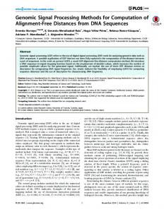
mately 200 milliseconds in both cases. Practically speaking, the pre-determined window width fixes the frequency resolution at 5 Hz; therefore, the interharmonic components that are between the bins spaced by 5 Hz primarily spill over into adjacent interharmonic bins and minimally spill into harmonic bins. Phase-locked loop (PLL) or other line frequency synchronization techniques should be used to reduce the errors in frequency components caused by spectral leakage effects. IEC Standards [1, 2] also introduce the concept of harmonic and interharmonic groups and subgroups, and characterize the waveform distortions with the amplitudes of these groupings over time. In particular, subgroups are more commonly applied when harmonics and interharmonics are separately evaluated. Figure 1 shows the IEC subgrouping of bins for 7th and 8th harmonic subgroups and for 7th interharmonic subgroup. The amplitude Gsg,n (Cisg,n ) of nth harmonic (interharmonic) subgroup is defined as the rms value of all its spectral components, as shown in Figure 1. Some of the authors of this paper have shown that in the IEC signal processing framework, a small error in synchronization causes severe spectral leakage problems and have proposed advanced signal processing methods that improve measurement accuracy by reducing sensitivity to desynchronization. The first method makes the IEC grouping compatible with the utilization of Hanning window (HW) instead of

EURASIP Journal on Advances in Signal Processing

Amplitude

2 Voltage spectrum time window of 200 ms

340 345 350 355 360 365 370 375 380 385 390 395 400 405 410 Frequency (Hz) Used for calculating Used for calculating Used for calculating 7th harmonic subgroup 7th interharmonic subgroup 8th harmonic subgroup

Figure 1: IEC grouping of “bins” for harmonic and interharmonic subgroups.

RW [3]. Another method, in the framework of synchronized processing (SP), uses a self-tuning algorithm, synchronizing the analysed window width to an integer multiple of the actual fundamental period [4]. Finally, a method in the framework of desynchronized processing (DP) is based on a double stage algorithm: harmonic components are filtered away before interharmonic evaluation [5–7]. Each of these methods adopts a technique of smoothing the results over aggregation intervals greater than the time window adopted for the analysis [1, 2]. The increase in complexity of the computational burden does not always correlate with increased accuracy of the results. Other authors of this paper have considered and developed alternative advanced methods [8–15]. In particular, the Prony- and ESPRIT-based methods (adaptive Prony method (APM) and adaptive ESPRIT method (AEM)) appear especially suitable for solving desynchronization (and time variation) problems warranting a very high level of accuracy. These methods approximate a sampled waveform as a linear combination of complex conjugate exponentials and are not characterized by a fixed frequency resolution. The computational burden of these methods may increase compared to DFT-based methods when high accuracy is required, but the increase is still reasonable, especially when using methods such as AEM. In this paper, the methods based on the use of the DFT in the IEC framework are summarized. Then, the methods based on Prony and ESPRIT theories are reviewed. Finally, the results of several numerical experiments are reported in order to compare the different methods in terms of accuracy. This paper is an extended and improved version of the paper presented previously at the PES meeting in 2006 [16]. 2.

DFT-BASED METHODS

In this section, several advanced methods, which use IEC guidelines and the DFT approach, are reviewed.

2.1.

Hanning windowing

The amount of spectral leakage interference depends strictly on the characteristics of the time window adopted to weight the signals before the spectral analysis; therefore, an appropriate choice can reduce the interference. The IEC Standard [2] refers to the RW, which is considered to be the window characterized by the narrowest main lobe (the best resolution among tones close in frequency), but with the highest and most slowly decaying side lobes (the worst interference caused by a strong tone on a weaker tone not close in frequency). The second type of interaction causes the greatest problems because of the amplitude difference between harmonic tones (which may vary in size by hundredths of a percent up to 100% of the fundamental tone) and interharmonic tones of interest (which are only a few thousandths of a percent of the size of the fundamental tone). Testa et al. [3] have shown how the Hanning window can be utilized instead of the rectangular window. In this case, only minor changes in the IEC procedure are required: one simply multiplies IEC group values by a factor equal to (2/3)1/2 . This reduces the leakage errors on the interharmonic groups by about one order of quantity as shown in Figure 2. It is worth noting that the errors are reported as a percentage of the amplitude of the close harmonic group and not of the interested interharmonic group, and are therefore very relevant. 2.2.

Result interpolation

Result interpolation allows one to estimate amplitude, frequency, and phase angle of signal components with great accuracy, starting from the results of a DFT performed at a given frequency resolution (i.e., −5 Hz). This method achieves results similar to those using a higher resolution analysis. The interpolation of a given tone is based on the assumption of negligibility of the spectral leakage effects caused by

3

10

10

1

1

δ Spectral amplitude

nth interharmonic group amplitude error (nth harmonic (%))

A. Bracale et al.

0.1

0.1 0.01

−1

−0.1

−0.01 0.01

0.1 nth harmonic frequency error (Hz)

1

1 L

0.01 M−3 L

M−1 M ν M+1 L L L Normalized frequency

Rectangular Hanning

Spectrum DFT

Figure 2: nth interharmonic group amplitude error versus nth harmonic frequency error: using RW (dotted line) and HW (dashed line).

Figure 3: Example of the spectrum (dashed line) and DFT components (•) of a signal.

the negative frequency replica and the other harmonic and interharmonic tones. These three conditions occur with a good approximation if a proper window is used. The authors selected the Hanning window because of its good spectral characteristics and the simplicity of the interpolation formulas. A brief review of the frequency domain interpolation technique is summarized below. A sampled and windowed single tone signal is considered:

being



s(k) = A sin 2π f



k + ϕ · w(k) with k = 0, 1, . . . , L − 1 fS (1)

with A being the tone amplitude, f the tone frequency, ϕ the phase angle, fS the sampling frequency, and w a generic window of length TW = L/ fS . Thus, the signal spectrum evaluated by means of the DFT on L points and neglecting the negative frequency replica equals 

A · exp( jϕ) i ·W −ν S(i) = 2j L



with i = 0, 1, . . . , L − 1, (2)

where ν = f / fS is the tone frequency normalized to the sampling frequency. In the presence of a small desynchronization between tone period and sampled time window, none of the DFT components matches the actual tone frequency as shown in Figure 3, where M is the order of the Mth DFT component and δ is the normalized frequency deviation from the actual normalized frequency. Adopting the Hanning window, approximated expres frequency f, and sions for the interpolated tone amplitude A, phase angle ϕ are     δ 1 − δ 2    , A = π S(M)  sin(π δ)

ϕ =

 ν=

M  + δ, L

π + ∠S(M) − M · π · δ 2

  S(M)

2−α |δ| = ,

α=    S M + sign(δ)  

1+α

(4)

 = sign(|S(M + 1)| − |S(M − 1)|). with sign(δ)

2.3.

Desynchronized processing

In the following section, the method proposed in [6]— that constitutes an example of desynchronized processing— is briefly recalled. It is based on harmonic filtering before the interharmonic analysis. Harmonic filtering A sampled and windowed time domain signal is considered: sw (k) = s(k) · w (k)

with k = 0, 1, . . . , L − 1,

(5)

where s is the signal and w the adopted window. It can be represented by the sum of two contributes, one harmonic and the other interharmonic:



sw (k) = sH (k) + sI (k) · w (k)

with k = 0, 1, . . . , L − 1. (6)

The evaluation of the amplitude AH n , of the normalized frequency νn , and of the phase ϕn , of each harmonic component gives  s H (k) =

n



AnH sin 2π νn k + ϕn



with k = 0, 1, . . . , L − 1. (7)

This contribution can be filtered from the original signal, for instance, in the time domain:  s I (k) = s(k) − s H (k)

with k = 0, 1, . . . , L − 1.

(8)

(3) The only way to eliminate spectral leakage effects is to have a very accurate estimation of the frequency, amplitude,

4

EURASIP Journal on Advances in Signal Processing

and phase angle of the harmonic components to be filtered. This can be accomplished by proper interpolation of the spectrum samples calculated by DFT [6, 7], such as that illustrated in Section 2.2. Interharmonic analysis Once sI (k) has been obtained, an interharmonic analysis can be performed with reduced harmonic leakage effects. The surviving harmonic leakage is given by εH (k) = sH (k) − s H (k)

with k = 0, 1, . . . , L − 1.

(9)

3.

PRONY- AND ESPRIT-BASED METHODS

In this section, Prony and ESPRIT methods are briefly recalled, and then advanced versions of these methods (adaptive Prony and ESPRIT methods) based on the use of proper time windows are analysed [8–16]. 3.1.

The Prony method

Let the signal sampled data [x(1) x(2) · · · x(N)] be approximated with the following linear combination of M complex exponentials1 [17]:

εH

This is generally different from zero. The lower is equal to the lower leakage effects. The use of a proper window w for the interharmonic analysis can reduce the residual harmonic leakage problems: sIw (k) = s I (k) · w (k)

with k = 0, 1, . . . , L − 1.

(10)

The choice of w must be made by considering additional aspects [3], such as interharmonic tone interaction and IEC grouping problems. Here, reference is made only to the HW.

x(n) =

M

k=1

f1r 2n 2n = (11) 10T1r 10 with T1r and f1r being the rated values of the system’s fundamental period and frequency, respectively. The technique generally implies a doubled number of FFT. It is worth noting that by using the same window for both the first and second stages, harmonic components can be directly filtered in the frequency domain due to the DFT linearity [6]. f S =

2.4. Smoothing of the results In the IEC standards [1, 2], it is highly recommended to provide a smoothing of the results obtained during the analyses. Smoothed results are derived from the components obtained in 200 milliseconds analyses as an average over 15 contiguous time windows, updated either every time window (approximately every 200 milliseconds) or every 15 time windows (about 3 s each). This procedure may affect the accuracy of the results when the desynchronization effects are remarkable in the 200- milliseconds window.

n = 1, 2, . . . , N,

(12)

where hk = Ak e jψk , zk = e(αk + jωk )Ts , k is the exponential code, Ts is the sampling time, Ak is the amplitude, ψk is the initial phase, ωk = 2π fk is the angular velocity, and αk is the damping factor. The problem is to find damping factors, initial phases, frequencies, and amplitudes solving the following nonlinear problem:

Accuracy and computational burden The accuracy is related to the filtering accuracy, which depends on the interpolation algorithms, the number of samples analysed, and interferences, such as those produced by interharmonic tones close to the harmonics (which need to be estimated and filtered). With regard to the computational burden, it is important to note that to achieve accuracy of equal or greater level than that of synchronized methods, an exact synchronization is not needed. It is therefore possible to choose a sampling frequency f  S , independent from the actual supply frequency, but still referring to its rated value. This allows one to acquire a number of samples using the power of two:

hk zk(n−1)

min

N

  x(n) − x(n)2 .

(13)

n=1

The Prony idea consists of first solving the following set of linear equations to find the damping factors and frequencies [17]: M

m=0

a(m)x(n − m) = 0,

(14)

where n = M + 1, M + 2, . . . , N. The (N − M) relations (14) constitute a linear equation system in M unknowns (i.e., the a(m) coefficients). If N = 2M, the system (14) can be solved in closed form since it represents an M-equation system with the same number of unknowns. In practice, the available samples are N > 2M, so an estimation problem has to be solved since the number of (14) are greater than the number of unknowns M (N − M > M). In this case, the M unknown coefficients a(m) can be obtained by minimizing the total error: ET =

N

M

n=M+1 m=0

a(m)x(n − m).

(15)

Once known the a(m) coefficients, the damping factors and the frequencies of each exponential are calculated by means of simple relations. The amplitudes and phases of each exponential are then calculated by solving a second set of linear equations linking these unknowns to the sampled data. 1

It has been shown that the best choice of the number M of complex exponentials for power system applications relies on using the minimum description length method [10].

A. Bracale et al.

5

3.2. The ESPRIT method The original ESPRIT algorithm [17–19] is based on naturally existing shift invariance between the discrete time series, which leads to rotational invariance between the corresponding signal subspaces. The assumed signal model is the following: x(n) =

M

k=1

( jωk n)

Ak ek

+ w(n),

(16)

where w(n) represents additive noise. The eigenvectors U of  x of the signal define two subthe autocorrelation matrix R spaces S1 and S2 (signal and noise subspaces) by using two selector matrices Γ1 and Γ2 : S1 = Γ1 U,

S2 = Γ2 U.

(17)

The rotational invariance between both subspaces leads to the equation S1 = ΦS2 ,

(18)

where ⎡

⎤

e jω1 0 · · · 0 ⎢ 0 e jω2 · · · 0 ⎥ ⎢ ⎥ Φ=⎢ . . .. ⎥ .. ⎢ . ⎥. . . ⎣ . . . ⎦ 0 0 · · · e jωM

(19)

The matrix Φ contains all information about M components’ frequencies. Additionally, the TLS (total least-squares) approach assumes that both estimated matrices S1 and S2 can contain errors and find the matrix Φ by means of minimization of the Frobenius norm of the error matrix. Amplitudes of the components can be found by properly using the auto x of the signal; alternatively, amplitudes correlation matrix R and phases (introduced in the signal model) can be found in similar way as with the Prony method by solving a second set of linear equations [20]. 3.3. The adaptive Prony and adaptive ESPRIT methods The basic idea of these methods consists in applying the Prony or ESPRIT methods to a number of “short contiguous time windows” inside the signal [11]; the widths of these short time windows are variable, and this variability ensures the best fitting of the waveform time variations. To select the most adequate short contiguous time windows, let us initially refer to the adaptive Prony method (APM) and consider the signal x(t) in a time observation period Tobs with L samples obtained using the sampling frequency fS = 1/Ts . The following mean square relative error can be considered: 2 εcurr

 2 L    1 x tk − x tk  = ,  2 L k=1 x tk

(20)

where tk = kTs (k = 1, 2, 3, . . . , L) and x(tk ) is given by (12). 2 The mean square relative error εcurr gives a measure of the fidelity of the model considered; in fact, it represents the mean square relative error of the model estimation. 2 By defining a threshold εthr (acceptable mean square relative error), it is possible to choose in the time observation period a short time window [ti , t f ] (or for fixed sampling frequency, a subset of the data segment length can be used) en2 2 ≤ εthr ). suring the satisfactory approximation (εcurr The main steps of the APM algorithm are the following: (i) select a starting short time window width Tmin ; (ii) apply the Prony method to the samples in the short time window to obtain the model parameters (amplitudes, damping factors, frequencies, and initial phases of the Prony exponentials); (iii) use the exponentials obtained in step (ii) to calculate 2 εcurr with (20); 2 2 (iv) compare εcurr with the threshold εthr and 2 2 (a) if εcurr ≤ εthr , store the Prony model exponential parameters and increase the short time window width (and then the subset of the data segment) 2 2 until εcurr ≤ εthr and t f ≤ Tobs , and then go to step (v); 2 2 (b) if εcurr is greater than the threshold εthr , increase the short time window width and go to step (vi);

(v) store the short time spectral components and select a new starting short time window width; (vi) compare t f with Tobs ; if t f is less than or equal to the observation period, go to step (ii); if t f is greater than Tobs , first calculate and store short time spectral components and then stop. It should be noted that in step (iv)(a), the short time win2 2 dow width is increased until the condition εcurr ≤ εthr is satisfied; the Prony model parameters remain fixed at the values that satisfy the criterion the first time. In this way, a nonnegligible reduction of the computational efforts arises, mainly in the presence of slight time-varying waveforms. The APM is generally characterized by very good accuracy in the assessment of waveform distortion in power systems, but its computational burden is certainly greater than the DFT methods; the computational efforts may be worthwhile when increased accuracy is required. Let us consider now the case of the adaptive ESPRIT method (AEM). As for APM, we apply the ESPRIT method to a number of “short contiguous time windows.” The main steps of the AEM algorithm include the following: (i) select a starting short time window width Tmin ;  x of the signal us(ii) estimate the autocorrelation matrix R ing the samples in the short time window;  x and then, matrices S1 (iii) calculate the eigenvalues of R and S2 ; (iv) estimate the matrix Φ; (v) calculate the eingenvalues of the matrix Φ and then, the frequencies of the exponentials;

6

EURASIP Journal on Advances in Signal Processing

(vi) calculate the amplitudes and arguments of the exponentials in a similar way to the Prony method, for assigned frequencies (step (v)) and damping factors2 ; (vii) use the exponential parameters obtained to calculate 2 εcurr with (20); 2 2 (viii) compare εcurr with the threshold εthr and 2 2 (a) if εcurr ≤ εthr , store the exponential parameters and increase the short time window width (and 2 then the subset of the data segment) until εcurr ≤ 2 εthr and t f ≤ Tobs , and then go to step (ix); 2 2 (b) if εcurr is greater than the threshold εthr , increase the short time window width and go to step (x);

(ix) store the short time spectral components and select a new starting short time window width; (x) compare t f with Tobs . If t f is less than or equal to the observation period Tobs , go to step (ii). If t f is greater than Tobs , first calculate and store short time spectral components, and then go to stop.

than APM. This is due to the fact that to better estimate  x a significant number of samples are necessary. the matrix R Therefore, enlarging the dimension of the short contiguous time windows and reducing the number of short contiguous time windows in the time observation period Tobs are often requirements for AEM. Moreover, since the APM model does not include the presence of noise, it generally requires a larger number M of complex exponentials to approximate the waveform in each of the short contiguous time windows. Finally, it should be noted that, the DFT-based methods are generally faster than the parametric methods, so that on the basis of our experience the rank of computational burden of the methods, from faster to slower, is (1) DFT-based methods; (2) adaptive ESPRIT method; (3) adaptive Prony method.

4. 3.4. Considerations The Prony- and ESPRIT-based methods have the following features: (i) the window width is free and only linked to the signal waveform characteristics; (ii) the adaptive version ensures the best fit of waveform variations by an optimal choice of the time window width; (iii) window width does not constrain the frequency resolution. The AEM is also characterized by excellent accuracy in the assessment of waveform distortion in power systems; its computational burden is greater than the DFT methods, but generally significantly lower than that required by APM. In practice, a comprehensive analytical comparison of AEM and APM computational efforts cannot be stated with general validity, since AEM and APM use different models to approximate the waveforms. Because of this, AEM and APM can be characterized not only by a different number of short contiguous time windows in the time observation period Tobs but also each short contiguous time window may have a different number M of complex exponentials used to approximate the waveform. However, some considerations can help demonstrate the reduced computational effort of AEM. These reduced computational efforts have been tested using several numerical applications performed on simulated and measured stationary/nonstationary waveforms, like the examples reported in Section 4. First, the AEM method generally requires fewer short contiguous time windows in the time observation period Tobs 2

Since in distortion assessment in power systems, the waveforms can be considered to be the sum of sinusoids, the damping factors value can be constrained to zero.

NUMERICAL EXPERIMENTS

Several numerical experiments were performed. In consideration of space, reference is made only to the results of four case studies. The examples were performed by utilizing the IEC normal approach (IEC-N) characterised by RW and TW = 200 milliseconds [1, 2], the interpolation technique (I-HW) described in Section 2.2 applied to the components obtained by DFT on 200 milliseconds using HW, the desynchronised procedure (IEC-DP) described in Section 2.3, and the adaptive Prony (APM) and adaptive ESPRIT methods (AEM) described in Section 3.3. All the data used in the experimental case studies were entered with the maximum allowable precision. The exact number of zeroes after the last significant cipher is not reported for the sake of simplicity. The results obtained are always reported in diagrams using two figures for DFT-based and high-resolution methods (APM and AEM). Two different scales for errors are used for high-resolution methods: left- side scale for APM and right-side scale for AEM. The sampling frequency for all the experiments and all the methods used is 5 kHz. The window width used is always Tw = 200 milliseconds for DFT-based methods. The window width varies from a minimum of 20 milliseconds (casestudies 1–3) to a maximum of 220 milliseconds (case study 4) for APM and AEM, but all results are presented with reference to 200 milliseconds [11], for ease of comparison of the methods. It should be noted that the number of samples can affect only the computational burden of DFT-based methods, in fact the FFT algorithm is faster when a number of samples that is a power of two is chosen. With reference to APM and AEM methods, the adaptive algorithm selects a variable number of samples (for each short contiguous time window) to fit at best the waveform considered; this number does not affect these methods. The acceptable mean square relative error for APM and AEM is ε = 1.0 · 10−15 .

A. Bracale et al.

7