strongly deteriorate the quality of the power supply voltage, Carbone R et al (1). Interharmonics are defined as non-integer harmonics of the main fundamental.
ADVANCED SIGNAL PROCESSING METHODS OF HARMONICS AND INTERHARMONICS ESTIMATION T Lobos, Z Leonowicz, J Rezmer, H-J Koglin* Wroclaw University of Technology, Poland
*Saarland University, Germany
INTRODUCTION The quality of voltage waveforms is nowadays an issue of the utmost importance for power utilities, electric energy consumers and also for manufactures of electric and electronic equipment. The voltage waveform is expected to be a pure sinusoidal with a given frequency and amplitude. Modern frequency power converters generate a wide spectrum of harmonic components, which deteriorate the quality of the delivered energy, increase the energy losses as well as decrease the reliability of a power system. In some cases, large converters systems generate not only characteristic harmonics, but also considerable amount of noncharacteristic harmonics and interharmonics, which may strongly deteriorate the quality of the power supply voltage, Carbone R et al (1). Interharmonics are defined as non-integer harmonics of the main fundamental under consideration. The estimation of the components parameters is very important for control and protection tasks. Estimation of the spectrum of discretely sampled processes is usually based on procedures employing the fast Fourier transform (FFT). This approach is computationally efficient and produces reasonable results for a large class of signal processes. In spite of the advantages there are several performance limitations of the FFT approach. The most prominent limitation is that of frequency resolution, i.e. the ability to distinguish the spectral responses of two or more signals. These procedures usually assumed that only harmonics are present and the periodicity intervals are fixed, while periodicity intervals in the presence of interharmonics are variable and very long. It is very important to develop better tools of interharmonic estimation to avoid possible damages due to their influence. A second limitation is due to windowing of the data. Windowing manifests itself as “leakage” in the spectral domain. These two limitations are particularly troublesome when analysing short data records. Short data records occur frequently in practice, because many measured processes are brief in duration or have slowly time-varying spectra that may be considered constant only for short record lengths. To alleviate the limitations of the FFT approach, many new spectral estimation methods have been proposed during the last decades, Cichocki A & Lobos T (3), Leonowicz Z (4), Lobos T et al (5). Advantages of the new methods depend strongly upon the signal-to-noise ratio (SNR). Even in those cases where improved spectral fidelity can be achieved, the computational effort of that alternative
methods may be significantly higher than FFT processing. Conventional FFT spectral estimation is based on a Fourier series model of the data, that is, the process is assumed to be composed of a set of harmonically related sinusoids. There are two spectral estimation techniques based on the Fourier transform: based on the indirect approach via an autocorrelation estimate (Blackman-Tukey), based on the direct approach via FFT operation (periodogram). Windowing of data makes the implicit assumption that the unobserved data outside the window are zero. A smeared spectral estimate is a consequence. If more knowledge about a process is available, or if it is possible to make a more reasonable assumption, one can select a model for the process that is a good approximation. It is then usually possible to obtain a better spectral estimate. Spectrum analysis becomes a three step procedure: to select a time series model, to estimate the parameters of the assumed model and finally to calculate the spectral estimate. The modelling approach enables to achieve a higher frequency resolution. There are three basic time series models: autoregressive (AR), moving average (MA) and autoregressive moving average (ARMA). Prony method is related to the autoregressive spectral estimation, Kay S M (6). The subspace frequency estimation methods rely on the property that the noise subspace eigenvectors of a Toeplitz autocorrelation matrix are orthogonal to the eigenvectors spanning the signal space. The model of the signal in this case is a sum of random sinusoids in the background of noise of a known covariance function. The eigenvectors spanning the noise space are the ones whose eigenvalues are the smallest and equal to the noise power. The earliest application of the property is the Pisarenko harmonic decomposition (PHD). The PHD method does not, itself, provide reliable frequency estimates. However, it has promoted a big interest in application of eigenanalysis to frequency estimation. One of the most important techniques, based on the concepts of subspaces is the min-norm method, Therrien C W (8). In the paper the frequencies of signal components are estimated using the Prony and min-norm methods. To investigate the ability of the methods several experiments were performed. Simulated current and current waveforms at the output of an industrial frequency converter were investigated. For comparison, similar experiments were repeated using the FFT.
PRONY METHOD Assuming the N complex data samples x[1],...,x[N ] the investigated function can be approximated by M exponential functions:
y[ n] =
M
∑ Ak e(α
k
+ j ω k )( n −1 )T p + jψ k
(1)
k =1
where n = 1, 2,..., N , Tp – sampling period, Ak – amplitude, α k – damping factor, ω k – angular velocity
ψ k – initial phase. The discrete-time function may be concisely expressed in the form
y[ n] =
M
∑ hk z kn−1
(2)
k =1
E noise = [eM +1 e M + 2
hk = Ak e j ψ k
K eN ]
(8)
Min-norm method uses one vector d for frequency estimation. This vector, belonging to the noise subspace, has minimum Euclidean norm and his first element equals to one. These conditions are expressed by the following equations T d = E noiseE*noise d
(9) d *T l = 1 Pseudospectrum defined with the help of d is defined as.
( )
Pˆ e j ω =
where
zk = e
N-M smallest eigenvalues of the correlation matrix (matrix dimension N>M+1) correspond to the noise subspace and M largest (all greater than σ 02 ) corresponds to the signal subspace. We define the matrix of eigenvectors:
1 *T
w d
2
=
1 w *T dd *T w
(10)
where w is an auxiliary vector is defined in (5).
(α k + jω k )T p
SIMULATED WAVEFORMS The estimation problem bases on the minimization of the squared error over the N data values:
δ =
N
∑ ε [n]
2
(3)
n =1
where
ε [n] = x[n] − y[n] = x[n] −
M
∑ hk z kn−1
(4)
k =1
This turns out to be a difficult non-linear problem. It can be solved using the Prony method that utilises linear equation solutions, Kay S M(6), Lobos T & Rezmer J(7) MIN-NORM METHOD The min-norm method involves projection of the signal vector: T s = 1 e jω i K e j( N −1)ω i (5) i
[
]
onto the entire noise subspace. We consider a random sequence x made up of M independent signals in noise.
x=
M
∑ Ai si + η ;
Ai = Ai e j φi
(6)
i =1
If the noise is white, the correlation matrix is
Rx =
∑ Ε {Ai Ai∗ }si sTi + σ 02I M
i =1
(7)
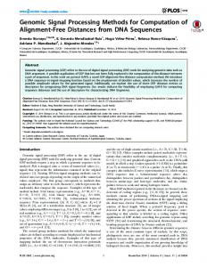
Several experiments were performed with the signal waveform described in Mattavelli P et al (2). The investigated signal is characteristic for DC arc furnace installations without compensation. It consists of basic harmonic (50 Hz) one higher harmonic (125 Hz), one interharmonic (25 Hz) and is additionally distorted by 5% random noise. The sampling interval was 0.5 ms. The signal was investigated using the Prony and minnorm methods. Both the methods enable us to detect all the signal components already using 100 sample (Fig. 1). For detection the 25 Hz component using the Fourier algorithm much more samples were needed. INDUSTRIAL FREQUENCY CONVERTER The investigated drive represents a typical configuration of industrial drives, consisting of a three-phase asynchronous motor and a power converter composed of a single-phase half-controlled bridge rectifier and a voltage source converter. The waveforms of the converter output current under normal conditions were investigated using the Prony, min-norm and FFT methods for the sampling windows equal to 20 ms (Fig.2) and 40 ms (Fig.3). The main frequency of the waveform was 40 Hz. When using the window 40 ms the estimation results are a little more accurate than for the window 20 ms. However, already the smaller window makes it possible to detect the main harmonic components. Using the Prony and min-norm methods the following harmonics have been detected: 5th , 7th , 17th , 19th , 25th , 35th and 41st . It is also possible to estimate the frequency of the fundamental component.
a 200
a 2.5
Magnitude [A]
Magnitude [A]
100 0
-100 -200
-2.5
0.05
0.005
0.01
0.015
Time [s]
280.7Hz
Magnitude [A]
25,48Hz
0
1
1003Hz
b 2
100
50
0
762.1Hz
0.04
125,0Hz
b 150
0
200
0
300
500
1000 Frequency [Hz]
500
1000 Frequency [Hz]
500
1000 Frequency [Hz]
762.2Hz
1500
100Hz
Magnitude [A]
10 -1
281.9Hz
c 50
40.4Hz
Frequency [Hz] 125.1Hz
Magnitude [A]
25,2Hz
c 1
100 50.03Hz
0
25
0
Magnitude [A]
1
1
1500
997Hz
d
286Hz
0
300
127Hz
21,5Hz
d 10
100 200 Frequency [Hz] 51,0Hz
0
771Hz
10 -4
37Hz
Magnitude [A]
0.02 0.03 Time [s]
40.3Hz
0.01
50,04Hz
0
Magnitude [A]
0
10-5 0.1 0
100 200 Frequency [Hz]
300
Figure 1: Voltage waveform at the output of a simulated DC arc furnace power supply installation (a); investigation results: Prony, M=30 (b); min-norm (c); FFT (d); fp =2000Hz, N=100.
0
1500
Figure 2: Current waveform at the output of a real frequency converter (a); investigation results: Prony M=40 (b); min-norm (c); FFT (d), N=100, fp =5000Hz
CONCLUSIONS It has been shown that a high-resolution spectrum estimation method, such as min-norm could be effectively used for parameter estimation of distorted signals. The Prony method could also be applied for estimation of the frequencies of signal components. The accuracy of the estimation depends on the signal distortion, the sampling window and on number of samples taken into the estimation process. Unfortunately, the computational effort of the highresolution methods is significantly higher than FFT processing. The proposed methods were investigated under different conditions and found to be variable and efficient tools for detection of all higher harmonics existing in a signal. They also make it possible the estimation of interharmonics.
0
-2.5
0
b 2
0.02 Time [s]
0.03
1644Hz
1001Hz
762.2Hz
REFERENCES
1
280.5Hz
Magnitude [A]
0.01 39.75Hz
Magnitude [A]
a 2.5
0 1500
1645Hz
1002Hz
1000 Frequency [Hz] 462.3Hz
280.9Hz
c 50 Magnitude [A]
500
39.98Hz
0
25
0
1646Hz
763Hz
1
1000 1500 Frequency [Hz]
1002Hz
Magnitude [A]
d
500
280Hz
40.5Hz
0
10-5 0
500
1000 Frequency [Hz]
1500
Figure 3: Current waveform at the output of a real frequency converter (a); investigation results: Prony M=80 (b); min-norm (c); FFT (d), N=200, fp =5000Hz
1. Carbone R et al, “Iterative harmonics and interharmonic analysis in multiconverter industrial systems”, 8th Int. Conference on Harmonics and Quality of Power, Athens (Greece), 1998, pp. 432-438. 2. Mattavelli P et al, “Analysis of interharmonics in DC arc furnace installation”, 8th Int. Conference on Harmonics and Quality of Power, Athens (Greece), 1998, pp. 1092-1099. 3. Cichocki A and Lobos T, “Artificial neural networks for real-time estimation of basic waveforms of voltages and currents”, IEEE Trans. Power Systems, vol. 9, no. 2, September 1994, pp 612-618. 4. Leonowicz Z et al, “Application of higher-order spectra for signal processing in electrical power engineering”, Int. Journal for Computation and Mathematics in Electronic Engineering COMPEL, 1998, vol. 17, no. 5/6, pp. 602-611. 5. Lobos T et al, “Power system harmonics estimation using linear least squares method and SVD”, 16th IEEE Instrumentation and Measurement Technology Conf., vol. 2, Venice (Italy), 1999, pp. 789-794. 6. Kay S M, ”Modern spectral estimation: theory and application”, Englewood Cliffs: Prentice-Hall, 1988, pp. 224-225. 7. Lobos T and Rezmer J, “Real time determination of power system frequency”, IEEE Trans. on Instrumentation and Measurement vol. 46, no 4, August 1997, pp. 877-881. 8. Therrien C W, “Discrete random signals and statistical signal processing”, Prentice-Hall, Englewood Cliffs, New Jersey, 1992, pp. 614-655. ACKNOWLEDGMENTS The authors would like to thank the Alexander von Humboldt Foundation (Germany) for its financial support, (Humboldt Research Award for Prof. T Lobos). This work was also partly supported by the State Committee for Scientific Research KBN (Poland).