Accurate Vision-based Vehicle Localization using Satellite ... - arXiv

Accurate Vision-based Vehicle Localization using Satellite Imagery Hang Chu

Hongyuan Mei

Mohit Bansal

Matthew R. Walter

Toyota Technological Institute at Chicago, Chicago, IL 60637, USA

arXiv:1510.09171v1 [cs.RO] 30 Oct 2015

{hchu,hongyuan,mbansal,mwalter}@ttic.edu

Abstract— We propose a method for accurately localizing ground vehicles with the aid of satellite imagery. Our approach takes a ground image as input, and outputs the location from which it was taken on a georeferenced satellite image. We perform visual localization by estimating the co-occurrence probabilities between the ground and satellite images based on a ground-satellite feature dictionary. The method is able to estimate likelihoods over arbitrary locations without the need for a dense ground image database. We present a rankingloss based algorithm that learns location-discriminative feature projection matrices that result in further improvements in accuracy. We evaluate our method on the Malaga and KITTI public datasets and demonstrate significant improvements over a baseline that performs exhaustive search.

I. I NTRODUCTION Autonomous vehicles have recently received a great deal of attention in the robotics, intelligent transportation, and artificial intelligence communities. Accurate estimation of a vehicle’s location is a key capability to realizing autonomous operation. Currently, many vehicles employ Global Positioning System (GPS) receivers to estimate their absolute, georeferenced pose. However, most commercial GPS systems suffer from limited precision and are sensitive to multipath effects (e.g., in the so-called “urban canyons” formed by tall buildings), which can introduce significant biases that are difficult to detect. Visual place recognition seeks to overcome this limitation by identifying a camera’s (coarse) location in an a priori known environment (typically in combination with map-based localization, which uses visual recognition for loop-closure). Visual place recognition, however, is challenging due to the appearance variations that result from environment and perspective changes (e.g., parked cars that are no longer present, illumination changes, weather variations), and the perceptual aliasing that results from different areas having similar appearance. A number of techniques have been proposed of late that make significant progress towards overcoming these challenges [3–15]. Satellite imagery provides an alternative source of information that can be employed as a reference for vehicle localization. High resolution, georeferenced, satellite images that densely cover the world are becoming increasingly accessible and well-maintained, as exemplified by the databases available via Google Maps [16] and the USGS [17]. Algorithms that are able to reason over the correspondence between ground and satellite imagery can exploit this availability to achieve wide-area camera localization [18–23]. In this paper, we present a multi-view learning method that performs accurate vision-based localization with the aid

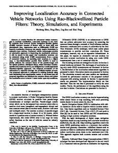
Fig. 1. Given a ground image (left), our method outputs the vehicle location (blue) on the satellite image (left), along the known vehicle path (orange).

of satellite imagery. Our system takes as input an outdoor stereo ground image and returns the location of the stereo pair in a georeferenced satellite image (Fig. 1), assuming access to a database of ground (stereo) and satellite images of the environment (e.g., such as those acquired during a previous environment visit). Instead of matching the query ground image against the database of ground images, as is typically done for visual place recognition, we estimate the co-occurrence probability of the query ground image and the local satellite image at a particular location, i.e., the probability over the ground viewpoint in the satellite image. This allows us to identify a more precise distribution over locations by interpolating the vehicle path with sampled local satellite images. In this way, our approach uses readily available satellite images for localization, which improves accuracy without requiring a dense database of ground images. Our method includes a listwise ranking algorithm to learn effective feature projection matrices that increase the features’ discriminative power in terms of location, and thus further improve localization accuracy. The novel contributions of this paper are: • We propose a strategy for localizing a camera based upon an estimate of the ground image-satellite image co-occurrence, which improves localization accuracy without ground image database expansion. • We describe a ranking-loss method that learns general feature projections to effectively capture the relationship between ground and satellite imagery. II. R ELATED W ORK Several approaches exist that address the related problem of localizing a ground image by matching it against an Internet-based database of geotagged ground images. These methods typically employ visual features [24, 25] or a combination of visual and textual (i.e., image tags) features [26].

These techniques have proven effective at identifying the location of query images over impressively large areas [24]. However, their reliance upon available reference images limits their use to regions with sufficient coverage (e.g., those visited by tourists) and their accuracy depends on the spatial density of this coverage. Meanwhile, several methods [27– 30] treat vision-based localization as a problem of image retrieval against a database of street view images. Majdik et al. [30] propose a method that localizes a micro aerial vehicle within urban scenes by matching against virtual views generated from a Google Street View image database. In similar fashion to our work, previous methods have investigated visual localization of ground images against a collection of georeferenced satellite images [18, 19, 21, 22]. Bansal et al. [19] describe a method that localizes street view images relative to a collection of geotagged oblique aerial and satellite images. Their method uses the combination of satellite and aerial images to extract building facades and their locations. Localization then follows by matching these facades against those in the query ground image. Meanwhile, Lin et al. [21] leverage the availability of land use attributes and propose a cross-view learning approach that learns the correspondence between features from ground-level images, overhead images, and land cover data. Viswanathan et al. [22] describe an algorithm that warps panoramic ground images to obtain a projected bird’s eye view of the ground that they then match to a grid of satellite locations. The inferred poses are then used as observations in a particle filter for tracking. Other methods [20, 23] focus on extracting orthographical texture patterns (e.g., road lane markings on the ground plane) and then match these observed patterns with the satellite image. These approaches perform well, but rely on the existence of clear, non-occluded visual textures. Meanwhile, other work has considered the related task of of visual localization of a ground robot relative to images acquired with an aerial vehicle [31, 32]. A great deal of attention has been paid in the robotics and vision communities to the related problem of visual place recognition [3–15]. The biggest challenges to visual place recognition arise due to variations in image appearance that result from changes in viewpoint, environment structure, and illumination, as well as to perceptual aliasing, which are both typical of real-world environments. Much of the work seeks to mitigate some of these challenges by using interest point detectors and descriptors that are robust to transformations in scale and rotation, as well as to slight variations in illumination (e.g., SIFT [33] and SURF [34]). Place recognition then follows as image retrieval, i.e., imageto-image matching-based search against a database (with various methods to improve efficiency) [27, 35–37]. While these methods have demonstrated reasonable performance despite some appearance variations, they are prone to failure when the environment is perceptually aliased. Under these conditions, feature descriptors are no longer sufficiently discriminative, which results in false matches (notably, when the query image corresponds to a environment location that is not in the map). When used for data association in a downstream

SLAM framework, these erroneous loop closures can result in estimator divergence. The FAB-MAP algorithm by Cummins and Newman [3, 5] is designed to address challenges that arise as a result of perceptual aliasing. To do so, FAB-MAP learns a generative model of region appearance using a bag-of-words representation that expresses the commonality of certain features. By essentially modeling this perceptual ambiguity, the authors are able to reject invalid image matches despite significant aliasing, while correctly recognizing those that are valid. Alternatively, other methods achieve robustness to perceptual aliasing and appearance variations by treating visual place recognition as a problem of matching image sequences [7– 10, 38], whereby imposing joint consistency reduces the likelihood of false matches. The robustness of image retrieval methods can be further improved by increasing the space of appearance variations spanned by the database [39, 40]. However, approaches that achieve invariance proportional to the richness of their training necessarily require larger databases to achieve robustness. Our method similarly learns a probabilistic model that we can then use for matching, though our likelihood model is over the location of the query in the georeferenced satellite image. Rather than treating localization as image retrieval, whereby we find the nearest map image for a given query, we instead leverage the availability of satellite images to estimate the interpolated position. This provides additional robustness to viewpoint variation, particularly as a result of increased separation between the database images (e.g., on the order of 10 m). Meanwhile, recent attention in visual place recognition has focused on the particularly challenging problem of identifying matches in the event that there are significant appearance variations due to large illumination changes (e.g., matching a query image taken at night to a database image taken during the day) and seasonal changes (e.g., matching a query image with snow to one taken during summer) [12, 14, 15, 39, 41, 42]. While some of these variations can be captured with a sufficiently rich database [39], this comes at the cost of requiring a great deal of training data and its ability to generalize is not clear [14]. McManus et al. [40] seek to overcome the brittleness of pointbased features to environment variation [7, 10, 43, 44] by learning a region-based detector to improve invariance to appearance changes. Alternatively, S¨underhauf et al. [14] build on the recent success of deep neural networks and eschew traditional features in favor of ones that can be learned from large corpora of images [45]. Their framework first detects candidate landmarks in an image using state-ofthe-art proposal methods, and then employs a convolutional neural network to generate features for each landmark. These features provide robustness to appearance and viewpoint variations that enables accurate place recognition under challenging environmental conditions. We also take advantage of this recent development in convolutional neural networks for image segmentation to achieve effective pixel-wise semantic feature extractors. Related to our approach of projection matrix learning is a

Stereo

Ground Image

Smoothed Color Edge Potential

Project

Depth Image

Neural Attributes

Satellite Image

Smoothed Color Edge Potential Neural Attributes

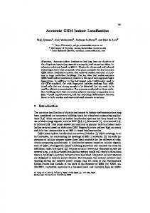
Ground-Satellite Dictionary Fig. 2.

Illustration of our ground and satellite feature dictionary learning process.

long history of machine learning research with ranking loss objective functions [46]. Our approach is also related to the field of multi-view learning [47], as we learn the relationship between ground and satellite image views. III. A PPROACH Our approach first constructs a ground-satellite feature dictionary that captures the relationship between the two views using an existing database from the area. Second, we learn projection matrices for the each of the two views so as to arrive at a feature embedding that is more locationdiscriminative. Given a query ground image, we then use the dictionary and the learned projections to arrive at a distribution over the location in georeferenced satellite images of the environment in which the ground image was taken. Next, we describe these three steps in detail. A. Ground-Satellite Image Feature Dictionary The role of the ground-satellite dictionary is to capture the relationships that exists between feature-based representations of ground images and their corresponding overhead view. Specifically, we define our ground-satellite image dictionary using three types of features. The first consists of pixel-level RGB intensity, which we smooth using bilateral filtering to preserve color transitions [48]. The second takes the form of edge potentials for which we use a structured forest-based method [49] that is more robust to non-semantic noise (as compared to classic gradient-based edge detectors) and can be computed in real-time. The third feature type we use are neural, pixel-wise, dense, semantic attributes. For these, we use fully-convolutional neural networks [50] trained on ImageNet [51] and finetuned on PASCAL VOC [52]. Next, we describe the process

by which we construct the ground-satellite dictionary, which we depict in Figure 2. For each ground image in the database, we identify the corresponding satellite image centered on and oriented with the ground image pose. We then compute pixel-wise features for both images. Next, we compute the ground image features gidict on a fixed-interval 2D grid (to ensure an efficient dictionary size), and project these sampled points onto the satellite image using the stereo-based depth estimate [53].1 Sampled points that fall outside the satellite image region are rejected. We record the satellite features corresponding to the remaining projected points, which we denote as sdict . We i repeat this process for all ground-satellite image pairs to form our one-to-one ground-satellite image feature dictionary. We also store dense satellite features even if they do not appear in the dictionary, so that they do not need to be recomputed during the localization phase. We store the dictionary with two k-d trees for fast retrieval. B. Location-Discriminative Projection Learning The goal of location-discriminative projection learning is to identify two linear projections Wg and Ws that transform the ground and satellite image features such that those that are physically close are also nearby in the projected space. Nominally, we can model this projection learning task as an optimization over a loss function that expresses the distance in location between each feature point and its nearest neighbor in the projected space. In the case of the ground 1 For the experimental evaluation, we use the stereo pair only to estimate depth. We only use images from one camera to generate the dictionary, learn the projections, and estimate pose.

Algorithm 1: Location-discriminative projection learning Input: {gidict }, {L(i)} Output: W 1: Initialize W = I and t = 0 2: for epi=1:M AX I TER do 3: for each i do 4: t = epi × imax + i   5: if fg (i, k ∗, W )− min fg (i, k, W )−m(i, k) > 0 k∈N (i)

then Compute ∂Lt as   ∂ fg (i, k ∗ , W ) − min fg (i, k, W ) /∂W

6:

k∈N (i)

7: 8: 9: 10: 11: 12: 13: 14:

Compute ∆Wt as A DAM({∂L0 , ∂L1 , . . . , ∂Lt }) [54] Update W ← W − ∆Wt end if end for if convergence then break end if end for

(a)

Fig. 3. Localization by (a) image-to-image matching using two-image reference database. By estimating the ground-satellite co-occurrence, our method (b) yields a more fine-grained distribution over the camera’s location, without the need for a larger ground image database. Iq denotes the db query ground image. Iidb denotes a database ground image, and Ldb i,0 . Li,1 and Ldb are the interpolated locations along the vehicle path. Our method is i,2 db able to evaluate localization possibilities of Ldb i,1 and Li,2 without knowing their ground images.

image, this results in a loss of the form X
Wg = arg min ∆L i, arg min fg (i, k, W ) , W

(1)

k∈N (i)

i

where ∆L(i, k) is the scalar difference in location (ignoring orientation for simplicity) between two feature points, N (i) is a neighborhood around feature i in feature space, and fg (i, k, W ) = kW gidict − W gkdict k2 . We consider a featurespace neighborhood for computational efficiency and have found a N (i) = 20 neighborhood to be effective in our reported experiments. A similar definition is used for Ws . In practice, however, this loss function is difficult to optimize. Instead, we treat the objective as a ranking problem and optimize over a surrogate loss function that employs the hinge loss,   X ∗ L= fg (i, k , W )− min fg (i, k, W )−m(i, k) (2) k∈N (i)

i

(b)

+

∗

where k = arg mink ∆L(i, k) is the nearest feature with regards to metric location, m(i, k) = ∆L(i, k) − ∆L(i, k ∗ ), and (x)+ = max(0, x) denotes the hinge loss. Intuitively, we would like the distance fg (i, k ∗ , W ) to be smaller than any other distance fg (i, k, W ) by a margin m(i, k). We minimize the loss function (2) using stochastic gradient descent with Adam [54] as the weight update algorithm. Algorithm 1 describes the process we use to learn a projection matrix, which is repeated twice for both Wg , and Ws . C. Localization In our final localization step, we compute the probability P (L|I q ) that a given query ground image I q was taken at a particular position and orientation L, where we interpolate the database locations along the vehicle path to get a larger

number of location candidates L (Fig. 3). In order to arrive at this likelihood, we first extract features for the query image I q and then retrieve the precomputed dense features for the satellite image associated with pose L. Next, we sample the query ground image features with a 2D grid and find their corresponding satellite image features by projecting using the query stereo image, as if I q was centered and oriented at pose L. After rejecting projected samples that lie outside the satellite image, we obtain a set of ground-satellite image feature pairs, where the nth pair is denoted as (gnq , sL n ). For each ground-satellite image feature pair, we evaluate their co-occurrence score according to the size of the intersection of their respective database neighbor sets in the projected feature space. To do so, we first transform the features to their corresponding projected spaces as Wg gnq and Ws sL n . Next, we retrieve their M -nearest neighbors, each for the transformed ground and satellite images, among the dictionary features projected into the projected space using the Approximate Nearest Neighbor algorithm [55]. The q retrieved neighbor index sets are denoted as {idm g (Wg gn )} m L and {ids (Ws sn )}. The Euclidean feature distances between q the query and database index m are denoted as {dm g (Wg gn )} m L and {ds (Ws sn )} for the ground and satellite images, respectively. A single-pair co-occurrence score is expressed as the consistency between the two retrieved sets −1 X  q q m2 L 1 score(sL dm , (3) n |gn ) = g (Wg gn ) · ds (Ws sn ) (m1 ,m2 )∈I q m L where I = {idm g (Wg gn )} ∩ {ids (Ws sn )} denotes all the (m1 , m2 ) pairs that are in the intersection of the two sets.

Fig. 4. Examples from the KITTI-City dataset that include (top) two ground images and (bottom) a satellite image with a curve denoting the vehicle path and arrows that indicate the poses from which the ground images were taken.

We then define the desired probability over the pose L for the query image I q as 1 X q P (L|I q ) = score(sL (4) n |gn ), C n where C is a normalizing factor. We interpolate the database vehicle path with Ldb i,j (Fig. 3) and infer the final location as that where P (L|I q ) is maximized. IV. E XPERIMENTAL R ESULTS We evaluate our method on the widely-used, publicly available KITTI [2] and Malaga-Urban [1] datasets. A. KITTI Dataset We conduct two experiments on the KITTI dataset. In the first experiment, we use five raw data sequences from the KITTI-City category. Together, these sequences involve 1067 total images, each with a resolution of 1242 × 375. The total driving distance for these sequences is 822.9 m. We randomly select 40% of the images as the database image set, and the rest as the query image set. Figure 4 provides examples of these images and the vehicle’s path. In the second KITTI experiment, we consider a scenario in which the vehicle initially navigates an environment and later uses the resulting learned database for localization when revisiting the area. We emulate this scenario using a long sequence drawn from the KITTI-Residential category, where we use the ground images from the first pass through the environment to generate the database, and images from the second visit as the query set. For the long KITTI-Residential sequences, we downsample the database and query sets at a rate of approximately one image per second to reduce the overlap in viewpoints, which facilitates the independence assumptions of FAB-MAP[5]. This results in 3654 total images (3376 images for the database and 278 images for the query), each with a resolution of 1241 × 376, with a total of 3080 m travelled by the vehicle (2847 m and 233 m

Fig. 5. Examples from the KITTI-Residential dataset that include (top) two ground images and (bottom) a satellite image. The yellow and cyan paths denote the vehicle path during the first and second visit, respectively. Green arrows indicate the pose from which the images were taken.

for the database and query, respectively). Figure 5 shows example ground images and the database/query data split. Note that while the ground-satellite dictionary is generated using images from the downsampled database, projection learning was performed using the full-framerate imagery along the database path. We evaluate three variations of our method on these datasets as a means of ablating individual components, and compare against two existing approaches, which serve as baselines. One baseline that we consider is a publicly available implementation of FAB-MAP [5],2 for which we use SURF features with a cluster-size of 0.45, which yields 2611 and 3800 bag-of-words for the two experiments, respectively. We consider a second baseline that performs exhaustive matching over a dense set of SURF features for image retrieval. We further refine these matches using RANSACbased [56] image-to-image homography estimation to identify a set of geometrically consistent inlier features. We use the average feature distance over these inliers as the final measurement of image-to-image similarity. We refer to this baseline as Exhaustive Feature Matching (EFM). The first variation of our method that we consider eschews satellite images and instead performs ground image retrieval using our image features (as opposed to SURF), which we refer to as Ours-Ground-Only (Ours-GO). The second ablation consists of our proposed framework with satellite images, but without learning the location-discriminative feature projection, which we refer to as Ours-No-Projection (Ours-NP). Lastly, we consider our full method that utilizes satellite images and all images along the database path for projection learning. For all methods, we identify the final position as a weighted average of the top three location matches. We also considered an experiment in which we include query images taken from regions outside those captured in our learned 2 https://github.com/arrenglover/openfabmap

(a) GPS trajectory error

(b) Reference image

(c) GPS-based match

(d) Correct match

Fig. 6. Data split for the Malaga sequence where yellow, cyan, and purple denote the database, revisit query, and the outside query set, respectively.

database and found that none of the methods produced any false positives, which we define as location estimates that are more than 10 m from ground-truth. TABLE I KITTI LOCALIZATION ERROR ( METERS ) Method

KITTI-City

FAB-MAP [5] EFM Ours-GO Ours-NP Ours-full

1.24 0.87 0.81 0.41 0.39

(0.69) (0.15) (0.07) (0.20) (0.22)

KITTI-Residential 2.29 1.18 1.13 0.62 0.42

(1.55) (0.91) (0.81) (0.33) (0.20)

Table I compares the localization error for each of the methods on the two KITTI-based experiments, with our method outperforming the FAB-MAP and EFM baselines. Ours-GO achieves lower error than the two SURF-based methods, which shows the effectiveness of our proposed features at discriminating between ground images, especially when there is overlap between images.3 Ours-NP further reduces the error by interpolating the trajectory between two adjacent ground database images (as described in Fig. 3) and evaluating ground-satellite co-occurrence probabilities, which brings in more localization information. Ours-full achieves the lowest error, which demonstrates the effectiveness of using re-ranking to learn the location-discriminative projection matrices. Note that Ours-NP and Ours-full use stereo to compute depth when learning the ground-satellite image dictionary, whereas FAB-MAP does not use stereo. B. Malaga-Urban Dataset We also evaluate our framework on the Malaga-Urban dataset [1], where we adopt the setup similar to KITTIResidential, using the first vehicle pass of an area as the database set, and the second visit as the query set. In addition, we also set aside images taken from a path outside the area represented in the database to evaluate each method’s ability 3 We note that this may violate independence assumptions that are made when learning the generative model for FAB-MAP [5].

Fig. 7. Deficiency of the ground-truth location tags in the Malaga dataset.

to handle negative queries. We used the longest sequence, Malaga-10, which contains 18203 images, each with a resolution of 1024 × 768. We downsample the database and query sets at approximately one frame per second. The total driving distance is 6.08 km, with 4.96 km for the database set, 583.5 m as the inside query set, and 534.3 m as the outside query set. Figure 6 depicts the data splits. Unlike the KITTI datasets, the quality of the groundtruth location tags in the Malaga dataset is relatively poor. Figure 7 conveys the deficiencies in the GPS tags provided with the data. Figure 7(a) shows a portion of the groundtruth trajectory, where the GPS data incorrectly suggests that the vehicle took an infeasible path through the environment. As further evidence, the GPS location tags suggest that the image in Figure 7(c) is 3.28 m away from the reference image in Figure 7(b) and constitutes the nearest match. However, the image in Figure 7(d) is actually a closer match to the reference image (note the white trashcan in the lower-right), despite being 5.48 m away according to the GPS data. Due to the limited accuracy of the ground-truth locations, we evaluate the methods in terms of place recognition (i.e., their ability to localize the camera within 10 m of the ground-truth location) as opposed to localization error. We compare the full version of our algorithm to the FABMAP and Exhaustive Feature Matching (EFM) methods as before. We set the bag-of-words size for FAB-MAP to 2589. We define true positives as images that are identified as inliers and localized within 10 m of their ground-truth locations. We picked optimal thresholds for each method based on the square area under their precision-recall curves (Fig. 8). Table II summarizes the precision and recall statistics for the different methods. The results demonstrate that our method is able to correctly classify most images as being inliers or outliers and subsequently estimate the location of the inlier images. The

1

method on multiple public datasets, which demonstrate its ability to accurately perform visual localization. Our future work will focus on the inclusion of additional features that enable learning with a smaller amount of data, and on learning general ground-to-satellite relationships that generalize across different environments.

0.9 0.8

Precision

0.7 0.6

B IBLIOGRAPHY 0.5 0.4 0.3 0.2

FAB-MAP EFM Ours-full

0.1 0

Fig. 8.

0

0.1

0.2

0.3

0.4

0.5 0.6 Recall

0.7

0.8

0.9

1

Precision-recall curve of different methods on the Malaga dataset. TABLE II O PTIMAL PRECISION - RECALL OF DIFFERENT METHODS . Method FAB-MAP [5] EFM Ours-full

Precision

Recall

49.3% 89.4% 90.2%

61.6% 43.6% 86.6%

EFM method achieves comparable precision, however the computational expense of doing exhaustive feature matching makes it intractable for real-time use in all but trivially small environments. Note that using only inlier images, the average location errors (with standard deviation) in meters when rough localization succeeds for FAB-MAP, EFM, and our method are 3.45 (2.16), 3.65 (2.21), and 3.33 (2.08), respectively. Although our method achieves better accuracy, it is difficult to draw strong conclusions due to the aforementioned deficiencies in the ground-truth data. We believe the improvement in accuracy of our method will be more significant if accurate ground-truth location tags are available, similar to what we have observed in our KITTI experiments. V. C ONCLUSION We presented a multimodal learning method that performs accurate visual localization by exploiting the availability of satellite imagery. Our approach takes a ground image as input and outputs the vehicle’s corresponding location on a georeferenced satellite image using a learned ground-satellite image dictionary embedding. We proposed an algorithm for estimating the co-occurrence probabilities between the ground and satellite images. We also described a rankingbased technique that learns location-discriminative feature projection matrices, improving the ability of our method to accurately localize a given ground image. We evaluated our

[1] J.-L. Blanco, F.-A. Moreno, and J. Gonz´alez-Jim´enez, “The m´alaga urban dataset: high-rate stereo and lidars in a realistic urban scenario,” Int’l J. of Robotics Research, vol. 33, no. 2, pp. 207–214, 2014. [2] A. Geiger, P. Lenz, C. Stiller, and R. Urtasun, “Vision meets robotics: the KITTI dataset,” Int’l J. of Robotics Research, 2013. [3] M. Cummins and P. Newman, “FAB-MAP: Probabilistic localization and mapping in the space of appearance,” International Journal of Robotics Research, vol. 27, no. 6, pp. 647–665, June 2008. [4] M. Park, J. Luo, R. T. Collins, and Y. Liu, “Beyond GPS: Determining the camera viewing direction of a geotagged image,” in Proc. Int’l Conf. on Multimedia, (ACM MM), 2010, pp. 631–634. [5] M. Cummins and P. Newman, “Appearance-only slam at large scale with fab-map 2.0,” Int’l J. of Robotics Research, vol. 30, no. 9, pp. 1100–1123, 2011. [6] W. Churchill and P. Newman, “Practice makes perfect? Managing and leveraging visual experiences for lifelong navigation,” in Proc. IEEE Int’l Conf. on Robotics and Automation (ICRA), Saint Paul, MN, May 2012, pp. 4525–4532. [7] M. J. Milford and G. F. Wyeth, “SeqSLAM: Visual route-based navigation for sunny summer days and stormy winter nights,” in Proc. IEEE Int’l Conf. on Robotics and Automation (ICRA), Saint Paul, MN, May 2012, pp. 1643–1649. [8] E. Johns and G.-Z. Yang, “Feature co-occurrence maps: Appearance-based localisation throughout the day,” in Proc. IEEE Int’l Conf. on Robotics and Automation (ICRA), Karsruhe, Germany, May 2013, pp. 3212– 3218. [9] N. S¨underhauf, P. Neubert, and P. Protzel, “Are we there yet? Challenging SeqSLAM on a 3000 km journey across all four seasons,” in Proc. Work. on Long-Term Autonomy at ICRA, Karsruhe, Germany, May 2013. [10] T. Naseer, L. Spinello, W. Burgard, and C. Stachniss, “Robust visual robot localization across seasons using network flows,” in Proc. Nat’l Conf. on Artificial Intelligence (AAAI), 2014. [11] S. Lynen, M. Bosse, P. Furgale, and R. Siegwart, “Placeless place-recognition,” in Proc. Int’l Conf. on 3D Vision (3DV), Tokyo, Japan, December 2014, pp. 303–310. [12] C. McManus, W. Churchill, W. Maddern, A. D. Stewart, and P. Newman, “Shady dealings: Robust, long-term visual localisation using illumination invariance,” in

[13]

[14]

[15]

[16] [17] [18]

[19]

[20]

[21]

[22]

[23]

[24]

[25]

[26]

[27]

Proc. IEEE Int’l Conf. on Robotics and Automation (ICRA), Hong Kong, May 2014, pp. 901–906. P. Hansen and B. Browning, “Visual place recognition using HMM sequence matching,” in Proc. IEEE/RSJ Int’l Conf. on Intelligent Robots and Systems (IROS), Chicago, IL, September 2014, pp. 4549–4555. N. S¨underhauf, S. Shirazi, A. Jacobson, F. Dayoub, E. Pepperell, B. Upcroft, and M. Milford, “Place recognition with ConvNet landmarks: Viewpoint-robust, condition-robust, training-free,” in Proc. Robotics: Science and Systems (RSS), Rome, Italy, July 2015. N. S¨underhauf, F. Dayoub, S. Shirazi, B. Upcroft, and M. Milford, “On the performance of ConvNet features for place recognition,” in Proc. IEEE/RSJ Int’l Conf. on Intelligent Robots and Systems (IROS), 2015. “Google Maps,” http://maps.google.com. United States Geological Survey, “Maps, imagery, and publications,” http://www.usgs.gov/pubprod/. N. Jacobs, S. Satkin, N. Roman, and R. Speyer, “Geolocating static cameras,” in Proc. Int’l Conf. on Computer Vision (ICCV), Rio de Janeiro, Brazil, October 2007. M. Bansal, H. S. Sawhney, H. Cheng, and K. Daniilidis, “Geo-localization of street views with aerial image databases,” in Proc. ACM Int’l Conf. on Multimedia (MM), Scottsdale, AZ, November 2011, pp. 1125–1128. T. Senlet and A. Elgammal, “A framework for global vehicle localization using stereo images and satellite and road maps,” in Proc. Int’l Conf. on Computer Vision Workshops (ICCV Workshops), 2011, pp. 2034–2041. T.-Y. Lin, S. Belongie, and J. Hays, “Cross-view image geolocalization,” in Proc. IEEE Conf. on Computer Vision and Pattern Recognition (CVPR), Portland, OR, June 2013, pp. 891–898. A. Viswanathan, B. R. Pires, and D. Huber, “Vision based robot localization by ground to satellite matching in GPS-denied situations,” in Proc. IEEE/RSJ Int’l Conf. on Intelligent Robots and Systems (IROS), 2014, pp. 192–198. H. Chu and A. Vu, “Consistent ground-plane mapping: A case study utilizing low-cost sensor measurements and a satellite image,” in Proc. IEEE Int’l Conf. on Robotics and Automation (ICRA), 2015. J. Hays and A. A. Efros, “IM2GPS: Estimating geographic information from a single image,” in Proc. IEEE Conf. on Computer Vision and Pattern Recognition (CVPR), Anchorage, AK, June 2008. Y.-T. Zheng, M. Zhao, Y. Song, and H. Adam, “Tour the world: Building a web-scale landmark recognition engine,” in Proc. IEEE Conf. on Computer Vision and Pattern Recognition (CVPR), Miami, FL, June 2009, pp. 1085–1092. D. J. Crandall, L. Backstrom, D. Huttenlocher, and J. Kleinberg, “Mapping the world’s photos,” in Proc. Int’l World Wide Web Conf. (WWW), Madrid, Spain, April 2009, pp. 761–770. G. Schindler, M. Brown, and R. Szeliski, “City-scale location recognition,” in Proc. IEEE Conf. on Computer

Vision and Pattern Recognition (CVPR), 2007. [28] A. R. Zamir and M. Shah, “Accurate image localization based on Google Maps Street View,” in Proc. European Conf. on Computer Vision (ECCV), Crete, Greece, September 2010, pp. 255–268. [29] D. M. Chen, G. Baatz, K. K¨oser, S. S. Tsai, R. Vedantham, T. Pylv¨an¨ainen, K. Roimela, X. Chen, J. Bach, M. Pollefeys, B. Girod, and R. Grzeszczuk, “Cityscale landmark identification on mobile devices,” in Proc. IEEE Conf. on Computer Vision and Pattern Recognition (CVPR), Providence, RI, June 2011, pp. 737–744. [30] A. L. Majdik, Y. Albers-Schoenberg, and D. Scaramuzza, “MAV urban localization from Google Street View data,” in Proc. IEEE/RSJ Int’l Conf. on Intelligent Robots and Systems (IROS), Tokyo, Japan, November 2013, pp. 3979–3986. [31] T. Stentz, A. Kelly, H. Herman, P. Rander, O. Amidi, and R. Mandelbaum, “Integrated air/ground vehicle system for semi-autonomous off-road navigation,” in Proc. of AUVSI Unmanned Systems Symp., July 2002. [32] A. Kelly, A. Stentz, O. Amidi, M. Bode, D. B. an A. Diaz-Calderon, M. Happold, H. Herman, R. Mandelbaum, T. Pilarski, P. Rander, S. Thayer, N. Vallidis, and R. Warner, “Toward reliable off road autonomous vehicles operating in challenging environments,” Int’l J. of Robotics Research, vol. 25, no. 5–6, pp. 449–483, May 2006. [33] D. G. Lowe, “Distinctive image features from scaleinvariant keypoints,” Int’l J. on Computer Vision, vol. 60, no. 2, pp. 91–110, 2004. [34] H. Bay, T. Tuytelaars, and L. Van Gool, “Surf: Speeded up robust features,” in Proc. European Conf. on Computer Vision (ECCV), 2006, pp. 404–417. [35] J. Wolf, W. Burgard, and H. Burkhardt, “Robust visionbased localization by combining an image-retrieval system with monte carlo localization,” Trans. on Robotics, vol. 21, no. 2, pp. 208–216, 2005. [36] F. Li and J. Kosecka, “Probabilistic location recognition using reduced feature set,” in Proc. IEEE Int’l Conf. on Robotics and Automation (ICRA), Orlando, FL, May 2006, pp. 3405–3410. [37] D. Filliat, “A visual bag of words method for interactive qualitative localization and mapping,” in Proc. IEEE Int’l Conf. on Robotics and Automation (ICRA), 2007, pp. 3921–3926. [38] O. Koch, M. R. Walter, A. Huang, and S. Teller, “Ground robot navigation using uncalibrated cameras,” in Proc. IEEE Int’l Conf. on Robotics and Automation (ICRA), Anchorage, AK, May 2010, pp. 2423–2430. [39] P. Neubert, N. S¨underhauf, and P. Protzel, “Appearance change prediction for long-term navigation across seasons,” in Proc. European Conf. on Mobile Robotics (ECMR), Barcelona, Spain, September 2013, pp. 198– 203. [40] C. McManus, B. Upcroft, and P. Newman, “Scene signatures: Localised and point-less features for locali-

[41]

[42]

[43]

[44]

[45]

[46]

[47] [48]

sation,” in Proc. Robotics: Science and Systems (RSS), Berkeley, CA, July 2014. W. Maddern, A. Stewart, C. McManus, B. Upcroft, W. Churchill, and P. Newman, “Transforming morning to afternoon using linear regression techniques,” in Proc. IEEE Int’l Conf. on Robotics and Automation (ICRA), Hong Kong, May 2014. S. M. Lowry, M. J. Milford, and G. F. Wyeth, “Transforming morning to afternoon using linear regression techniques,” in Proc. IEEE Int’l Conf. on Robotics and Automation (ICRA), Hong Kong, May 2014, pp. 3950– 3955. C. Valgren and A. J. Lilienthal, “SIFT, SURF and seasons: Long-term outdoor localization using local features,” in Proc. European Conf. on Mobile Robotics (ECMR), Freiburg, Germany, September 2007. A. J. Glover, W. P. Maddern, M. J. Milford, and G. F. Wyeth, “FAB-MAP + RatSLAM: Appearance-based SLAM for multiple times of day,” in Proc. IEEE Int’l Conf. on Robotics and Automation (ICRA), Anchorage, AK, May 2010, pp. 3507–3512. O. Russakovsky, J. Deng, H. Su, J. Krause, S. Satheesh, S. Ma, Z. Huang, A. Karpathy, A. Khosla, M. Bernstein et al., “Imagenet large scale visual recognition challenge,” Int’l J. on Computer Vision, pp. 1–42, 2014. L. Hang, “A short introduction to learning to rank,” IEICE TRANSACTIONS on Information and Systems, vol. 94, no. 10, pp. 1854–1862, 2011. C. Xu, D. Tao, and C. Xu, “A survey on multi-view learning,” arXiv preprint arXiv:1304.5634, 2013. K. N. Chaudhury, “Acceleration of the shiftable algorithm for bilateral filtering and nonlocal means,” IEEE

[49]

[50]

[51]

[52]

[53]

[54]

[55]

[56]

Trans. on Image Processing, vol. 22, no. 4, pp. 1291– 1300, 2013. P. Doll´ar and C. L. Zitnick, “Structured forests for fast edge detection,” in Proc. Int’l Conf. on Computer Vision (ICCV), 2013, pp. 1841–1848. J. Long, E. Shelhamer, and T. Darrell, “Fully convolutional networks for semantic segmentation,” in Proc. IEEE Conf. on Computer Vision and Pattern Recognition (CVPR), 2015. J. Deng, W. Dong, R. Socher, L.-J. Li, K. Li, and L. Fei-Fei, “ImageNet: A Large-Scale Hierarchical Image Database,” in Proc. IEEE Conf. on Computer Vision and Pattern Recognition (CVPR), 2009. M. Everingham, L. V. Gool, C. K. Williams, J. Winn, and A. Zisserman, “The Pascal visual object classes (VOC) challenge,” Int’l J. on Computer Vision, vol. 88, no. 2, pp. 303–338, 2012. K. Yamaguchi, D. McAllester, and R. Urtasun, “Efficient joint segmentation, occlusion labeling, stereo and flow estimation,” in Proc. European Conf. on Computer Vision (ECCV), 2014, pp. 756–771. D. Kingma and J. Ba, “Adam: A method for stochastic optimization,” in Proc. Int’l Conf. on Learning Representations (ICLR), 2015. S. Arya, D. M. Mount, N. S. Netanyahu, R. Silverman, and A. Y. Wu, “An optimal algorithm for approximate nearest neighbor searching fixed dimensions,” J. of the ACM, vol. 45, no. 6, pp. 891–923, 1998. M. Fischler and R. Bolles, “Random sample consensus: A paradigm for model fitting with applications to image analysis and automated cartography,” Comm. of the ACM, vol. 24, no. 6, pp. 381–395, June 1981.