Achieving accurate and context-sensitive timing for code optimization§ R. Clint Whaley1,∗,† , Anthony M. Castaldo1 1 University of Texas at San Antonio, Department of Computer Science, 6900 N Loop 1604 West, San Antonio, TX 78249
key words:
timers; timing; benchmarking; cache flushing; kernel optimization; ATLAS
SUMMARY Key computational kernels must run near their peak efficiency for most high performance computing (HPC) applications. Getting this level of efficiency has always required extensive tuning of the kernel on a particular platform of interest. The success or failure of an optimization is usually measured by invoking a timer. Understanding how to build reliable and context-sensitive timers is one of the most neglected areas in HPC, and this results in a host of HPC software that looks good when reported in papers, but which delivers only a fraction of the reported performance when used by actual HPC applications. In this paper we motivate the importance of timer design, and then discuss the techniques and methodologies we have developed in order to accurately time HPC kernel routines for our well-known empirical tuning framework, ATLAS.
1.
INTRODUCTION
In high performance computing (HPC), there are many applications for which no amount of compute power is “enough”. A key example of this is in scientific simulation, where an increase in compute speed will allow the scientist to increase the accuracy of the model, rather than solving the same problem in less time. Many HPC applications share this characteristic: the time that the application runs is always as long as the scientist can afford, and so extra speed translates to more detailed or accurate problem solving.
∗ Correspondence
to: R. Clint Whaley, University of Texas at San Antonio, Department of Computer Science, 6900 N Loop 1604 West, San Antonio, TX 78249 † E-mail:
[email protected] § This is a preprint accepted for publication in Software: Practice and Experience, John c Wiley & Sons Ltd Contract/grant sponsor: National Science Foundation CRI grant; contract/grant number: SNS-051504
ACCURATE AND CONTEXT-SENSITIVE TIMING
1
Such applications are written so that their computational needs can be serviced to the greatest possible degree by building-block computational libraries. This reduces the ongoing optimization tasks to tuning a modest number of widely used kernel operations, rather than tuning each HPC application individually. Some of the operations of interest include matrix multiply (main kernel for dense linear algebra), sparse matrix-vector multiply (sparse linear algebra), and fast Fourier transforms (FFTs). Therefore, there are a variety of commercial and academic libraries dedicated to optimizing these types of kernels, and the literature contains many publications which discuss them. More particularly, there are a host of papers each year devoted to code transformations for performance optimization, both in compiler and HPC journals. As far as we can determine, however, there is little or no discussion (beyond a few scanty details available in textbooks) of how to accurately measure the performance improvements that have actually been achieved by these optimizations. The best source of this kind of information is probably papers on various benchmarking systems, such as [11, 7, 21]. However, since these types of publications are mainly about a particular benchmark suite, they typically discuss timing issues only tangentially, without providing the full details necessary to employ any given techniques outside of their narrow operation/platform/set of assumptions. This is unfortunate, and represents an ongoing problem for both researchers and users of HPC libraries. The reason is that most timers† used by researchers are extremely na¨ıve, and thus fail to take account of important information such as cache state, so that often the “tuned” code produced using a na¨ıve timer for optimization decisions is no faster than untuned code when used in the application, despite the timer having shown a large speedup. Therefore, the literature is regrettably replete with performance numbers that are realized by few, if any, actual applications. This problem has recently become acute, with the rise of packages that adapt critical performance kernels to given architectures using an automated timing/tuning step. Such efforts include domain-specific optimizers, which include PHiPAC [1], FFTW [2, 4, 3], ATLAS [15, 16, 17, 19, 18], SPIRAL [10, 8], and OSKI [14], as well as research on iterative compilation [13, 12, 6, 20]. This type of research is all typified by making code transformation decisions based on timings taken on a platform of interest. Since optimization choices are based on these timings, it becomes critical that the timers are calling the computational kernels in the way in which the applications call them. 1.1.
Understanding the scope of the problem
Figure 1 shows the performance of ATLAS’s dot product kernel on a 2.4Ghz Core2Duo processor, timed using two different methods. The red line with triangles shows the results reported by a na¨ıve timer (such a timer can be seen in Figure 3(b)) which preloads the cache, whereas the blue line with squares shows the results as reported by a timer which ensures that the operands are not cache-resident. At the beginning of the curve, the unflushed timer
† By ‘timers’ we mean programs written to measure kernel performance; when we need to refer to the OSprovided hooks that read various system clocks, we will use the phrase ‘system timers’
c 2008 John Wiley & Sons, Ltd. Copyright Prepared using speauth.cls
Softw. Pract. Exper. 2008; 00:0–0
2
R. C. WHALEY AND A. M. CASTALDO
reports more than 3.5 times faster performance than the flushed timer on the same kernel. The unflushed timings within this region time performance when running the kernel with all the operands preloaded to the L1 data cache. After N = 2048 the operands will no longer fit in the 32Kb L1 data cache, and so N = 2048 starts a new plateau, with the unflushed version running roughly three times faster than the flushed version. This second plateau corresponds to running the kernel with all operands preloaded to the L2 cache. However, once N reaches roughly 200, 000, the operands begin to exceed the L2 cache size and so the unflushed timings exhibit a precipitous drop-off in performance, until at the end of the timing range the flushed and unflushed timers produce nearly identical results. We stress we are timing exactly the same kernel throughout, so this graph demonstrates the magnitude of the problem on even a simple kernel like dot-product: If there is no good reason to assume operands will be in L1, a timer that preloads the operands to L1 (or any level of cache) can report extremely misleading timings. These results are fairly typical when contrasting flushed and unflushed timers: the unflushed timers show large performance losses on cache boundaries, which results in small problems achieving greater performance than large problems. Flushed results typically show a pattern of steady performance improvement until an asymptotic speed is reached. This reflects what we expect to see: that larger problems tend to get better perforFigure 1. Dot product results from cache flushed mance, as transformations with and unflushed timers overheads (eg., unrolling) amortize their startup costs more completely, and large-scale optimizations such as blocking kick in. In the case of dot product we see a flat flushed curve, because dot product, which is a simple operation with only a few key optimizations, has essentially already fully amortized its optimizations at our starting problem size. Our dot product kernel is not particularly well optimized for this platform, and the unflushed/flushed ratio can grow even more extreme for other kernels/implementations/ architectures. Therefore, we see that the results reported can be significantly different depending on how the timer is implemented. This leads to the question of whether tuning using the wrong timing methodology will produce a differently optimized kernel, or if they will in fact be the same. The answer is that indeed, the timing methodology has a strong effect on what the best optimization parameters are. In [20] we showed that having the operands in- or outof cache strongly changed both the type and degree of beneficial transformations for even the simplest of kernels. Less formally, consider two simple optimizations: data prefetch and load/use software pipelining. When data is in the cache, neither one of these optimizations may give any advantage at all, and indeed due to overheads, might cause a slowdown.
c 2008 John Wiley & Sons, Ltd. Copyright Prepared using speauth.cls
Softw. Pract. Exper. 2008; 00:0–0
ACCURATE AND CONTEXT-SENSITIVE TIMING
3
If the data is out-of-cache, and the operation is bus-bound, then these may be the most important optimizations that can be applied. More generally, in-cache timings will stress the importance of computational optimizations, and out-of-cache timings will stress the importance of memory optimizations. Unfortunately, memory is several orders of magnitude slower than modern processors, and so a kernel that is completely optimal computationally may run no faster than an unoptimized kernel when called with operands that are not preloaded to the cache. Therefore, we see that if we empirically tune the kernel using the in-cache numbers, we will be able to report massive speedups in a paper, but any user calling our kernel with out-of-cache data may experience no speedup at all over unoptimized code. Even worse, by tuning for the in-cache case, we may have produced a kernel that is far less efficient than we could have produced using our current tuning framework, merely because our na¨ıve timer showed (a) Using a timer with flushing that crucial memory optimizations gave no benefit. To put some teeth behind the idea that timing with the wrong context can cause an automatic tuning framework to underperform its potential, we installed ATLAS’s double precision matrix multiply (DGEMM) twice on a 1.35Ghz UltraSPARC IV. For both installs, we refused architectural defaults (which allow ATLAS to skip parts of the automatic tuning by using previously saved values), and ran a complete automatic tuning of DGEMM from the ground up. In (b) Using a timer without flushing the first install, ATLAS was allowed to flush the cache as usual Figure 2. Performance of resulting ATLAS DGEMM in all timings, and in the secon an UltraSPARC IV when the automatic tuning ond install, we turned off cache step uses cache flushing (squares), and when cache flushing completely. Figure 2 shows flushing is turned off (triangles) the performance of the resulting automatically-tuned kernel. In figure 2(a), we measure the performance using a timer which flushes the cache, and in Figure 2(b)
c 2008 John Wiley & Sons, Ltd. Copyright Prepared using speauth.cls
Softw. Pract. Exper. 2008; 00:0–0
4
R. C. WHALEY AND A. M. CASTALDO
we measure the same two kernels using a timer which does no cache flushing. These figures have similar asymptotic peaks, since large enough operands overflow the cache, but as we have seen before, the timer without flushing reports inflated numbers when the operands are cache-contained. We see that with the cache flush timer (Figure 2(a)), the performance curve of the DGEMM tuned with cache flushing on (blue squares) behaves as expected: a relatively smooth rise in performance until an asymptotic peak is reached (the performance drop at N=800 results from a poor matrix partitioning brought on by our L2 cache blocking). The install without flushing (red triangles) does not. The primary difference in these two differently-tuned kernels is that, without flushing, the ATLAS framework picks bad blocking factors for the L1 and L2 caches, and thus as the cache is exceeded performance drops off. This results in the DGEMM tuned without flushing having its asymptotic peak reduced by almost half when compared with DGEMM tuned with cache flushing. The timings are much more volatile when measured with a timer without flushing, as in Figure 2(b). These early drops in performance represent the kicking in of new optimizations that have yet to amortize their cost (eg., the performance drop between N=40 and N=60 for the no-flush-tuned DGEMM is due to the matrix size exceeding the L1 blocking factor for the first time). These optimizations cause a performance loss on in-cache data (where they did not when our timer flushed the cache), since blocking, for instance, does not improve in-cache performance. This provides a further demonstration of the problem of timing things in-cache: it shows blocking, which is critical for out-of-cache performance, to be a performance loss unless you are lucky enough to time a problem large enough to do the appropriate amount of self-flushing. One interesting thing to note is that the DGEMM tuned using timers without flushing actually wins for small problems. This is because smaller L1 blocking factors provide better performance for smaller problems, and tuning in-cache causes ATLAS to choose a blocking factor that is ill-tuned for large problems (where blocking is truly important). This is why the asymptotic performance of the DGEMM tuned without flushing is only a little more than half of the DGEMM tuned with flushing. Note that ATLAS’s main DGEMM algorithm is presently designed so that we must use only one L1 blocking factor regardless of problem size, and so the install chooses to optimize for asymptotic performance at a slight cost to small problems. We plan to extend our DGEMM to handle multiple blocking factors, and with this in place, the cache-flushed DGEMM will win across the entire range, since the smaller blocking factor shows up as an advantage for small problems regardless of the timing methodology used during tuning. Further, DGEMM is a kernel that reuses the operands in the cache if they fit; in other kernels that don’t have this native reuse, we would find that for out-of-cache operands, the cache-flush-tuned kernel would win throughout the entire range. The performance loss due to failure to time appropriately when tuning will vary by architecture, kernel, and tuning framework. The present case is not very extreme, in that the two installs differ mainly on what blocking factors are used. The ATLAS framework always blocks; another framework might apply blocking only when it shows a win. In-cache timings might not show any win at all from blocking, which would result in a calamitous asymptotic performance loss. There are a host of options that work like this: for instance in-cache timing might show software prefetch to be of little use even when it is critical for
c 2008 John Wiley & Sons, Ltd. Copyright Prepared using speauth.cls
Softw. Pract. Exper. 2008; 00:0–0
ACCURATE AND CONTEXT-SENSITIVE TIMING
5
out-of-cache performance, or if prefetch does help for in-cache performance, it is likely that the prefetch distance will be poorly tuned for out-of-cache usage. Since some computational optimizations also have memory optimization impact (eg., instruction scheduling), it is possible for installs using different timing methodologies to choose completely different computational kernels, which could further impact true performance. Given these results, it should be clear that timer design has a profound effect on the ultimate performance of the kernel being tuned. Thus it is critical that automated tuning frameworks, which cannot rely on human judgment to bridge the gap between timer and application usage, pay particular attention to proper timer design. 1.2.
Addressing the problem
We have seen that the timing methodology used can have a strong effect on the best way to optimize a kernel, particularly in regards to handling the cache. Since differing methodologies can lead to widely varying results, understanding whether users typically call the kernel with in- or out-of-cache data becomes overwhelmingly important. It is critical to understand that it is kernel usage, not problem size, that dictates whether you wish to flush the cache: if a user calls the kernel with a problem small enough to fit into the cache, but his application does not have it in cache at the time of the call (eg., the kernel operands have been evicted by other memory access, or were brought in outside the cache, as with some types of direct memory access), then indeed you must still flush the cache if you are to capture the context of this use. In practice, it need not be all-or-nothing: a kernel may be typically called with one operand in the L2 cache and another in main memory, etc. What is important is to be sure to tune the library to the important case, and this demands that timers need to be sophisticated enough to recreate all important calling contexts. Having flexible timers can have other benefits as well. For instance, we often measure many computational transforms using in-cache timings, and then begin memory transform tuning starting from this computationally optimized code using out-of-cache timings. Therefore, in this paper we describe the timing methodologies we developed in order to support ATLAS’s empirical tuning. Our approach is to choose a default timing method that we believe represents the majority of our users (out-of-cache timings with paged-in kernel code), but build our timers flexibly enough that a user with a different context could tune them for that as well. Therefore, this paper should serve as a tutorial on how to build a timer that is accurate and adaptable enough to be used to make optimization decisions in the real world. Concrete examples often provide the best mechanism for understanding such applied concepts, and so we will show actual code that utilizes these methods to time a simple dot product kernel. In order to get started, Figure 3(a) shows the simple dot product kernel, while Figure 3(b) shows the type of na¨ıve dot product timer that a typical programmer might write. In examining this timer, notice that we initialize the operands, which will bring them into any cache large enough to hold them. We then immediately start the timing, which will therefore be with in-cache data (assuming the vectors fit in some level of cache). In §3 and §4 we will discuss how to control what operands are allowed to be in various levels of the cache. The second thing to notice about this na¨ıve timer is that the kernel is called only once, which may
c 2008 John Wiley & Sons, Ltd. Copyright Prepared using speauth.cls
Softw. Pract. Exper. 2008; 00:0–0
6
R. C. WHALEY AND A. M. CASTALDO
double dotprod( const int N, const double *X, const double *Y) { int i; double dot=0.0; for (i=0; i= 0; i--) x[i] = my_drand(); x=X; y=Y; k=0; t0 = my_time(); for (i=0; i < nrep; i++) { dot += alpha*dotprod(N, X, Y) if (++k != nset) { x -= setsz; y -= setsz; } else {x=X;y=Y;k=0;alpha = -alpha;} } time = (my_time()-t0)/((double)nrep); free(vp);
op2 ... opN op1 op2 ... opN .. . .. . op1
c a c h e f l u s h a r e a
op2 ... opN
13
?
(a) Cache flushing area diagram
(b) Mult. call dot product timer
Figure 6. Cache flushing for multiple kernel invocations
Therefore, our approach to timing a problem that is below timer resolution is to time multiple kernel invocations (where the number of kernel invocations is selected so that the interval being timed is comfortably above clock resolution) that are self flushing. To do this, an area of memory that is large enough to overflow the chosen cache level to the appropriate degree (as discussed in §3) is allocated. This memory is subdivided into working sets required by the kernel, as shown in Figure 6(a), where a working set is all the operands required by the kernel (in dot product the working set would be the two input vectors X and Y, plus the scalar dot, which would have no effect on performance and is therefore ignored). After a given kernel invocation, we simply move to a new working set before making the second call, and since this cache flush area is large enough to flush the desired level of the cache, by the time we must reuse a working set, it has been evicted from the cache due to conflict and capacity misses caused by accessing the other working sets. We abbreviate this technique as MultCallFlushLRU. In practice we refine this simple concept somewhat in order to minimize the effects of hardware prefetch. We initialize the entire cache flush area in reverse order, and then start timing with work set N . We know that our dot product kernel accesses the memory in leastto-greatest address order, and so we move amongst working sets in the opposite direction. Since the operation being timed accesses the working set in a loop, all but the shortest vector lengths will allow any hardware prefetch units to detect the least-to-greatest access pattern, and so any hardware prefetch will fetch the beginning portion of the working set that we used last time through the repetition loop, rather than what we will use on the next iteration.
c 2008 John Wiley & Sons, Ltd. Copyright Prepared using speauth.cls
Softw. Pract. Exper. 2008; 00:0–0
14
R. C. WHALEY AND A. M. CASTALDO
Given enough working sets, it might be possible to traverse the working sets in a random walk to more fully guard against smart prefetch units figuring out the pattern. In practice, we typically don’t need to allocate that many working sets, and the algorithm given above seems to produce the desired result on the machines that ATLAS has used over the years. We show this ‘backwards-traversal-of-sets’ timer for dot product in Figure 6(b). As before, we see that we allocate the flush area, and we make sure that its length is a multiple of our working set size (the working set for dot product is two N -length vectors, which we store as setsz). We then initialize the data in reverse order (greatest-to-least), and since this area’s size has been chosen to overflow the cache, working set N ’s space should be evicted by the time we have initialized work set 1. We then set our pointers to point to the appropriate areas in working set N , and begin the repetition loop. It is important to keep all the non-kernel code in this loop as efficient as possible, since the time for these additional instructions is being added to the time that is reported for kernel calls. Therefore, we have only one if, which is computationally efficient and optimized for the frequent case so that normally we simply decrement the vector pointers by the set size, and then reset them when we have used all working sets. Note that alpha is used to guard against overflow, which if it occurred, could completely invalidate the timings. This is discussed in more detail in §5. Note that in the discussion so far we have assumed contiguous and regularly accessed data. The reliability of this algorithm will be reduced if these assumptions do not hold. If your data is strided (i.e. accessed elements aren’t contiguous but have gaps, or strides, between them), then the safest alternative is to base the size of your flush area on the number of elements addressed (i.e., if op1 is a strided N-length vector with accessed elements separated by 31 unaccessed elements, then you count op1 as taking up only N elements for flushing, even though the space taken up by the operand (in elements) is N × 32), rather than the space taken up by the operand (these two quantities are the same for contiguous storage). Note that with large strides, the efficiency of the flush is likely to go down, as capacity misses are likely to be replaced by conflict misses, which therefore may no longer be flushing the oldest data (eg., imagine the operand stride is the exact cache size in a direct-mapped cache: all N accesses will only overwrite one cache line). Similarly, this technique is likely to have reduced effectiveness if you cannot predict operand access. Imagine timing an operation like ”find a given value in a list”: in one call it might only examine the first element of an N -length operand! In this case, MultCallFlushLRU will either need to be adapted to the details of your algorithm, or another timing method employed. 4.1.
Modifications for partial cache flush
Since this self-flushing timer is based on the same cache concepts as the OneCallFlushLRU timer, the MultCallFlushLRU timer can also be used to flush only certain caches by the appropriate setting of the cacheKB variable. At the cost of a slight complication, this timing methodology can also allow for the flushing of only certain of the operands in the working set. The easiest way to do this is to allocate each operand for which we wish to be able to change the flush characteristics in its own cache flush area. We can then use a variable (compile- or run-time) to control whether we move through a particular cache flush area, or leave the pointer unchanged across iterations of the repetition loop. This may complicate our repetition
c 2008 John Wiley & Sons, Ltd. Copyright Prepared using speauth.cls
Softw. Pract. Exper. 2008; 00:0–0
ACCURATE AND CONTEXT-SENSITIVE TIMING
15
loop slightly, as the operand pointers must be updated individually. When we split the cache flush area so that each operand has its own, we may be able to reduce the individual size due to the access pattern within the loop. If this is the case, initializing each operand in turn may no longer completely flush the cache, so that we must either initialize all the used flush areas in the appropriate order (i.e. in the order they would be used in the repetition loop), or additionally use one of the methods shown in Figure 5 to force the initial flush.
5.
TIMER REFINEMENTS
In this section we briefly mention a few refinements that the programmer should be aware of when writing a high quality timer. This includes guarding against overflow and underflow in floating point data, and avoiding unpredictable system-level events such as lazy page zeroing and instruction loading (all of these terms are described below). Further, §5.5 discusses how timers can guarantee a particular memory alignment for operands, and why this can be important. Finally, §5.6 discusses some of the pitfalls and techniques for performing timings on shared memory parallel machines. 5.1.
Turning off CPU throttling for reliable timing
Most modern CPUs (including desktop machines), now have the capability to run at slower speeds in order to save power and reduce heat dissipation. This is known as CPU throttling, and it is critical that it be switched off if reliable timings are to be obtained. Detecting whether throttling is enabled is usually not difficult, as your timings will vary widely, and be much lower than expected. We have never gotten reliable results with CPU throttling enabled using any timer. The reason is that between kernel invocations, the timer doesn’t keep the CPU busy, and so the clock rate is cycled down, and then the kernel timing begins, which ups the load. Unfortunately the OS will not recognize the increased load at the exact same place in each run, so that every timing (of even the same kernel) will show essentially a random speed somewhere between the CPUs slowest and fastest clock rate, depending on factors that defy a priori prediction. Obviously, the problem becomes even more acute for parallel timings, where load is even less evenly distributed. Therefore, when running timings, CPU throttling must be switched off (note that for parallel timings, it is critical to turn off CPU throttling on all processors that might be used in the parallel timing). The method of turning off CPU throttling will vary by OS and machine. For many PCs, it can be turned off in the BIOS. Most OSes also have some mechanism. For instance, Fedora Linux uses the command: /usr/bin/cpufreq-selector -g performance to turn off CPU throttling for your first processor. For parallel machines, you must add the -c # to switch off throttling on every processor of interest (eg., -c 3 added to the above will switch off throttling on the fourth system processor, while the above command alone would behave the same if you added -c 0).
c 2008 John Wiley & Sons, Ltd. Copyright Prepared using speauth.cls
Softw. Pract. Exper. 2008; 00:0–0
16
R. C. WHALEY AND A. M. CASTALDO
5.2.
Guarding against over/underflow (RangeGuard):
Overflow (underflow) occurs when a number grows too large (small) to be stored using the restricted number of exponent bits available in floating point storage. Many machines handle overflow and underflow arithmetic (even denormalized or gradual underflow) in software, rather than in hardware. This fact means that arithmetic experiencing overflow or underflow will possibly run hundreds or thousands of times slower than normal computation. Therefore, if the timer is calling a kernel multiple times in order to get the timing interval above a certain resolution, it is important to guard against creating conditions that can lead to overflow or underflow. In any timer that repeatedly adds into the same output data, it is possible that a buildup of magnitude could cause overflow, particularly if the results are all the same sign. Similarly, any time the same result is reused across many multiplications, there is a risk of overflow (for numbers > 1 in absolute value) or underflow (for numbers < 1 in absolute value). It is possible to take several actions to guard against this, including varying the input in known ways (eg. input1 produces the negation of input0), changing the accumulating operation slightly (eg. on one call, add results in, and on the second subtract results), or always using separate output locations for each call (this method is often ruled out by storage costs when the output is a large vector or matrix). Figure 6(b) shows an example of changing the accumulation to guard against overflow. We are performing a series of dot products using a fixed number of invariant input vectors, and if the number of dot products is large enough, this could eventually cause overflow on the output scalar dot. In order to guard against this, we say dot += alpha*dotprod(...), rather than dot += dotprod(...) (Note that dot = dotprod() is not safe, in that if the compiler figures out that dotprod is a pure function, the loop can be replaced with a single call). Alpha is initially set to 1, but every time we traverse all the working sets, we reverse the sign of alpha, so that in the second traversal of the working set we subtract off the same numbers that we added in during the previous traversal. Therefore, as long as we can make one traversal of the working set without overflow, this timer will not overflow (actually, due to error caused by aligning the mantissas of the numbers, it is possible to construct a case where overflow could still happen, but in practice it should not). We ensure that overflow doesn’t happen for particularly long vectors by using input vectors that produce mixed sign data (so that the dot product is not always increasing in magnitude). Of course, we could rule out any problem with overflow by initializing all vectors to zero, but since it is possible some systems might handle this case more optimally than normal arithmetic (particularly architectures that do floating point in software) we prefer to use the alpha method instead. 5.3.
Lazy page zeroing (Page0Guard):
If the kernel being timed accesses operands which are not initialized by the timer before invoking the kernel (eg., workspace or output operands), it becomes critical to access each page of data before making the call. This is because many OSes do “lazy zeroing” of pages. For security reasons, memory allocated from the system (which can include pages freed from another user’s processes) must be overwritten before the allocating process is allowed to read
c 2008 John Wiley & Sons, Ltd. Copyright Prepared using speauth.cls
Softw. Pract. Exper. 2008; 00:0–0
ACCURATE AND CONTEXT-SENSITIVE TIMING
17
it. In lazy zeroing, the newly-allocated page is not zeroed, but is protected so that any access of the page raises an exception. Then, when the allocating process attempts to access the unzeroed page, an exception handler which zeroes the entire page is called. The advantage of this scheme is in avoiding the overhead of zeroing pages that are never accessed, and postponing some overhead which allows user programs to begin operation faster. However, when this is allowed to happen during kernel timing, the timer will report a cost (which for some kernels is quite substantial) that only occasionally occurs: if the needed space is already available in user-space, no extra cost is seen, but if the allocation requires using a system page, then the cost is added. Whether this occurs depends not only on the particular OS and environment settings, but also on the initial state of the process’s memory. The easiest fix for this is to be sure to access all memory that the kernel uses before calling the kernel, even when no initialization is required.
5.4. Effects of instruction load (InstLdGuard): Instruction load time can cause strong variance in kernel timings, particularly on the first call to the kernel. This is because most OSes load only a few pages of an executable at the beginning of the program and load the remaining pages only if and when they are needed. Thus, if the kernel isn’t allocated to the same page as the kernel timer, the first call to the kernel may have disk access time added to its cost. Whether the kernel must be loaded from disk depends on a host of factors that defy a priori prediction, and therefore in the interest of getting repeatable timings it is advisable to ensure that the kernel routine is in memory before beginning timings, which can be done by making a dummy kernel call before commencing the timings. In our own work, we make the dummy call to force the load of the kernel’s instruction page before doing any cache flushing, so that the data-cache flushing that is performed will also flush any shared caches. Most machines have instruction and data share all caches except the L1 cache, which is almost always separate. This means that small kernels will probably be retained in the L1 cache. Unfortunately, we have not discovered a portable way to reliably flush the instruction cache, particularly when calling the kernel multiple times. Preloading the I-cache is a more realistic assumption in general than preloading the data cache, since it is usually a smaller cost and most kernels are called multiple times in loops where it is highly likely that the kernel will be retained in some level of the cache. However, in those cases where the kernel in question is called only once and has low complexity (so that the computational costs do not dominate the instruction load), this may cause timings to be too optimistic. This could theoretically lead to poor optimization. For example, it might incorrectly show that an optimization that increases code size (eg. loop unrolling) is a performance win, when in fact for the way this kernel is called it is a loss due to the increased instruction loads. In our own work, most of the kernels have a large enough computational and data complexity compared to their code size that this cost is not very important, and so in the interest of getting repeatable timings we ensure that the kernel is in memory rather than on disk before beginning timings.
c 2008 John Wiley & Sons, Ltd. Copyright Prepared using speauth.cls
Softw. Pract. Exper. 2008; 00:0–0
18
R. C. WHALEY AND A. M. CASTALDO
5.5.
Enforcing memory alignment on operands (MemAlign)
For some kernels on some architectures, the memory alignment of the operands can have a drastic effect on performance. Probably the most important example of this is SSE-enabled kernels on the x86. SSE (Intel’s SIMD vectorization ISA extension) operates on vectors that are 16 bytes in length. Most C libraries, however, have memory allocation routines that return memory only 8-byte aligned (this matches the size of C’s double, which is the longest unmodified native C type). Like any data type, the SIMD vectors must be aligned to their native length to avoid the possibility of cache line splits, which can roughly double the cost of a load. Since malloc will, roughly speaking, return a 16-byte aligned address on only half of the calls, this can cause timing of codes which benefit from 16-byte alignment to vary widely in an unpredictable way. More specifically, a memory-bound SSE operation such as vector copy might actually run twice as fast when the timer gets “lucky” and allocates memory that is 16-byte aligned, and then in a second call gets “unlucky” and run at the cache line split speed. The key to avoiding these problems is to program alignment adaptability into the timer. Again, context sensitivity demands the ability to vary the timer’s behavior, since some users may typically call the kernel with aligned data, some unaligned, and some a mixture. Therefore, the timer needs to be able to generate both aligned and purposely misaligned operands (i.e. a kernel might have different performance for an 8-byte aligned address that is not allowed to be 16-byte aligned, than one that is 16-byte aligned). The kernel can then be tuned in multiple phases, where first the aligned kernel is optimized, and then this kernel is adapted to handle misaligned operands as efficiently as possible. Forcing a given alignment on memory is simple in theory, but fairly complicated to get right in practice. Therefore Figure 7 shows wrappers that can be used to force alignment restrictions on memory allocations. In these routines, align is a nonzero variable that indicates what byte boundary the memory should be aligned to, while misalign indicates a greater alignment that the allocation should not be allowed to be aligned to (eg., passing align=4 and misalign=16 asks for memory aligned to a 4-byte boundary that is not allowed to be aligned to a 16-byte boundary). If misalign=0, then no maximal alignment is to be forced. The aligning wrappers amalloc and afree shown in Figure 7 allocate extra space in front of the user’s requested area, which serves two purposes: First, the over-allocation provides room to position a pointer that is aligned as the user has requested. We call this the “user pointer”. However, when we call the free routine to release the memory, we must provide the pointer received from the call to malloc, which we designate the “original pointer”. So the extra space also stores the original pointer. In practice we must align it on a pointer boundary; but for any given user pointer the location of the original pointer is deterministic, so afree needs only the user pointer. The memory overhead we incur is (2*sizeof(void*)+align) on allocations that do not require forced misalignment, and (2*sizeof(void*)+2*align) for allocations that do require forced misalignment. The (2*sizeof(void*)) portion ensures enough space to store the original pointer on a pointer-aligned boundary. If misalignment is needed we first set the user pointer to the earliest possible aligned position, then if that position also happens to be aligned on the prohibited boundary, we add the alignment increment to the user pointer,
c 2008 John Wiley & Sons, Ltd. Copyright Prepared using speauth.cls
Softw. Pract. Exper. 2008; 00:0–0
ACCURATE AND CONTEXT-SENSITIVE TIMING
void afree(void *P) { size_t n = ((size_t) P) - sizeof(void*); n = n - (n % sizeof(void*)); void **A = ((void**) n); free(*A); } // END *** afree *** /******************************************/ void *amalloc(size_t size, int align, int misalign) { void *P; size_t extra, n, s; extra=2*sizeof(void*)+align; if (misalign > align) P = malloc(size+extra+align); else P = malloc(size+extra); // If malloc fails, we fail. if (P == NULL) return(NULL); // (continued in next column)
19
// We allocated space. Move n past our // ’extra’ header space. n = ((size_t) P)+extra; n = n-(n%align); // Back up to align it. // n is aligned. Check if TOO aligned. if (misalign > align) { if ((n%misalign) == 0) n += align; // Force misalignment. } //------------------------------------// n is the finished user pointer. Now // back up from ’n’ to a valid address // to store the original malloc void*, // and save it for afree() to use. //------------------------------------s = n - sizeof(void*); // Get space. s = s - (s%sizeof(void*)); // Align it. *((void**) s) = P; // Store original. return( (void*) n); // Exit with new. } // END *** amalloc ***
Figure 7. Wrapper code forcing a memory allocation to be aligned on an align-byte boundary, but not allowed to be aligned to a misalign-byte boundary. If misalign=0, then no maximal alignment is set. If it is nonzero, then align must be < misalign.
which will preserve the alignment but force the requested misalignment (hence the necessity of (2*align)). 5.6.
Cache flushing for shared memory parallel timings
So far this paper has been concentrated on getting reliable serial timings. To extend these timing techniques to shared memory parallel operations, it is necessary to understand the cache state of all processors in the machine. The techniques we have been discussing should be adequate to flush any shared cache, at least those shared caches where one processor can access the entire shared cache. However, caches local to the processors that are used for computation, but which do not run the timing thread (which does flushing), must be handled explicitly. How this is handled will differ depending on the timer method being used. In the following discussion, assume that Np is the number of processors possessed by the shared memory parallel computer, and p is the number of processors being used (1 < p ≤ Np ). For the single-invocation timers discussed in §3, there is sometimes no adaptation required for parallel operation. Since only the master (timer) process has initialized the operands, the operands should only be in cache on that process’s processor, and the normal flush mechanism will ensure that no processors’ cache is preloaded with the data. More sophisticated timers,
c 2008 John Wiley & Sons, Ltd. Copyright Prepared using speauth.cls
Softw. Pract. Exper. 2008; 00:0–0
20
R. C. WHALEY AND A. M. CASTALDO
however, are likely to use the operands repeatedly, even when each timing interval contains only a single kernel invocation. The most common reason is the need to perform multiple timings (each one of which consists of only one call to the kernel) of the kernel in order to get reliable timings, as described in §2.1. In these cases, the timer will often perform the kernel timing several times in a row on the same data. Since the prior kernel call will have brought some operands into the local caches of other processors, it will no longer suffice to flush only the master thread’s cache. At first glance, it may appear sufficient to simply re-initialize the data, thus invalidating the other processors caches, but this assumes a certain shared memory cache protocol (i.e. this wouldn’t work on some systems with snoopy caches). Therefore the most straightforward adaptation is to simply spawn the appropriate cache flush loop of Figure 5 to all processors which might be used during the timed computation. If the timer cannot control which processors are used in the computation, it will be necessary to flush all processors in the system, even if the kernel uses only a subset of the available processors. To see why, imagine that the kernel selects to use only three processors for the given problem, and on the first invocation the threads were spawned to processors {0,3,5} of an 8 processor shared memory computer. We now wish to flush the cache before invoking the kernel a second time, and we spawn the flush loop using three threads, which happen to go to processors {0,2,4}, thus leaving processors 3 and 5 with preloaded data, which will cause timing variations if these processors are used in a subsequent kernel invocation. Therefore, if the processors used when threading cannot be precisely controlled, it will by necessary to spawn the cache flush loop to all Np processors, even if p < Np . For the multiple-invocation timer given in Figure 6, adapting to parallel timing requires us to increase the cache flush area. In an operation like dot product, each processor of a p-thread of parallel implementation (assuming one thread per processor) will need to access only a setsz p data, where setsz is the size of the working set of the operation. Since the idea of this timing method is to not reuse data until it has been discarded from cache, we must therefore increase the size of our flush space by a factor of p (and, in the rare case of heterogeneous processors, choose our flush size based on the largest cache). There are some operations that do not exactly divide their working sets by p (for instance, perhaps they divide an output operand, but not the input), in which case a smaller increase will provide adequate cache flushing. Increasing by p should always provide a safe flush, though it may be too large an area (i.e., either it flushes a larger cache that we hoped to preload, or it is so large that the allocation fails). Again, if we cannot be sure the same p processors are used in each invocation, we will have to set p of the above discussion to Np (and insist that only one thread be spawned to each processor), rather than allowing p to be based on the number of threads spawned by the kernel being timed.
6.
FUTURE WORK
We are aware of two areas that could affect timer design that we have not yet investigated in enough detail to provide meaningful guidance. The first is the effects of NUMA (Non-Uniform Memory Access) shared memory architectures (such as AMD’s recent machines) on sharedmemory parallel timings. In a NUMA system, timings may change based what processor owns the operand memory initially vs. what processors are assigned to operate on the operands. In
c 2008 John Wiley & Sons, Ltd. Copyright Prepared using speauth.cls
Softw. Pract. Exper. 2008; 00:0–0
ACCURATE AND CONTEXT-SENSITIVE TIMING
21
order to address this adequately, we will need a literature search on NUMA architectures and tuning, and then likely case studies on various architecture/OS combinations will be needed to quantify any problems that arise for timings in the real world. The second area we have not yet investigated enough to have meaningful insight into is the effects of using a more rigorous statistical approach on both timing accuracy and installation time. As we saw in §2.1, ATLAS presently takes a few samples, and then returns the minimum (median) for wall (CPU) time. Our experience is that this leads to adequate results. However, we have seen that when competing transformations are close in performance, it may fail to tease out the difference, and select an inferior optimization due to timing error. There should be several ways we could improve this approach using basic statistics and possibly a higher number of samples. One approach would be to treat all timings as means, and continue sampling until a more formal statistical test distinguishes between them or concludes they are identical. The standard is a T-Test on the difference between two means, and complete details are available in most statistics textbooks, including [?]. If we are statistically certain at some given confidence level that the difference in mean timings is non-zero, we can choose the better of the two transformations. Likewise we can determine a confidence interval for the mean difference in timings, and if it is narrow enough conclude the optimizations are effectively equal (which would leave us free to make the choice on another metric, such as instruction size, resource consumption, ease of further transformation, etc). These statistical methods require computing the sample variances in the two timings. Intuitively, the variance in timings reflects what else is happening in the computing environment during the timings. Therefore, if the timings for the two methods are alternated back-to-back it seems reasonable to use the tests in which the variances are assumed to be equal, otherwise we suggest using the tests in which the variances are assumed to be different. To fully analyze this problem we would have to identify a pool of statistical approaches which might improve timer accuracy, and then compare and contrast them with the present approach for both accuracy and install time.
7.
SUMMARY
This paper first introduced and demonstrated the importance of timing methodology in optimization, including highlighting its critical importance for automatic tuning frameworks. The following sections provided detailed discussions of the techniques we have found necessary to obtain high enough quality timings that automated optimization decisions can be based on them in the real world. We have not found much mention of these techniques in the literature, though many are, of course, direct applications of basic architecture information. It seems likely that many benchmark authors and hand tuners have probably used and reinvented similar techniques historically, though in our discussions and reading we have found no mention of the technique discussed in §4 that we developed in our original ATLAS work. At any rate, both discussions at conferences and the publication record firmly establish that many researchers are either unaware of the importance of taking careful timings, or do not know precisely how to perform them, and so we believe publishing these techniques explicitly will be a strong contribution to the field of optimization in general, and automated empirical optimization in particular.
c 2008 John Wiley & Sons, Ltd. Copyright Prepared using speauth.cls
Softw. Pract. Exper. 2008; 00:0–0
22
R. C. WHALEY AND A. M. CASTALDO
REFERENCES 1. J. Bilmes, K. Asanovi´ c, C.W. Chin, and J. Demmel. Optimizing Matrix Multiply using PHiPAC: a Portable, High-Performance, ANSI C Coding Methodology. In Proceedings of the ACM SIGARC International Conference on SuperComputing, Vienna, Austria, July 1997. 2. Franz Franchetti, Stefan Kral, Juergen Lorenz, and Christoph Ueberhuber. Efficient utilization of simd extensions. Accepted for putblication in IEEE special issue on Program Generation, Optimization, and Adaptation, 2005. 3. M. Frigo and S. Johnson. FFTW: An Adaptive Software Architecture for the FFT. In Proceedings of the International Conference on Acoustics, Speech, and Signal Processing (ICASSP), volume 3, page 1381, 1998. 4. M. Frigo and S. G. Johnson. The Fastest Fourier Transform in the West. Technical Report MIT-LCSTR-728, Massachusetts Institute of Technology, 1997. 5. John Hennessy and David Patterson. Computer Architecture, A Quantitative Approach. Morgan Kaufmann Publishers, Inc., San Francisco, California, 1990. 6. T. Kisuki, P. Knijnenburg, M. O’Boyle, and H. Wijsho. Iterative compilation in program optimization. In CPC2000, pages 35–44, 2000. 7. Larry McVoy and Carl Staelin. lmbench: portable tools for performance analysis. In ATEC’96: Proceedings of the Annual Technical Conference on USENIX 1996 Annual Technical Conference, pages 23–23, Berkeley, CA, USA, 1996. USENIX Association. 8. J. Moura, J. Johnson, R. Johnson, D. Padua, M. Puschel, and M. Veloso. Spiral: Automatic implementation of signal processing algorithms. In Proceedings of the Conference on High-Performance Embedded Computing, MIT Lincoln Laboratories, Boston, MA, 2000. 9. M. O’Boyle, N. Motogelwa, and P. Knijnenburg. Feedback assisted iterative compilation. In LCR, 2000. 10. Markus Pushel, Jose Moura, Jeremy Johnson, David Padua, Manuela Veloso, Bryan Singer, Jianxin Xiong, Franz Frenchetti, Aca Cacic, Yevgen Voronenko, Kang Chen, Robert Johnson, and Nick Rizzolo. Spiral: Code generation for dsp transforms. Accepted for putblication in IEEE special issue on Program Generation, Optimization, and Adaptation, 2005. 11. A.J. Saavedra, R.H.; Smith. Measuring cache and tlb performance and their effect on benchmark runtimes. Transactions on Computers, 44(10):1223–1235, Oct 1995. 12. P. van der Mark, E. Rohou, F. Bodin, Z. Chamski, and C. Eisenbeis. Using iterative compilation for managing software pipeline – unrolling tradoffs. In SCOPES99, 1999. 13. Paul van der Mark. Iterative compilation. Master’s thesis, Leiden Institute of Advanced Computer Science, 1999. 14. Richard Vuduc, James W. Demmel, and Katherine A. Yelick. OSKI: A library of automatically tuned sparse matrix kernels. In Proceedings of SciDAC 2005, Journal of Physics: Conference Series, San Francisco, CA, USA, June 2005. Institute of Physics Publishing. (to appear). 15. R. Clint Whaley and Jack Dongarra. Automatically Tuned Linear Algebra Software. Technical Report UT-CS-97-366, University of Tennessee, December 1997. http://www.netlib.org/lapack/lawns/lawn131.ps. 16. R. Clint Whaley and Jack Dongarra. Automatically tuned linear algebra software. In SuperComputing 1998: High Performance Networking and Computing, 1998. CD-ROM Proceedings. Winner, best paper in the systems category. http://www.cs.utsa.edu/~whaley/papers/atlas_sc98.ps. 17. R. Clint Whaley and Jack Dongarra. Automatically Tuned Linear Algebra Software. In Ninth SIAM Conference on Parallel Processing for Scientific Computing, 1999. CD-ROM Proceedings. 18. R. Clint Whaley and Antoine Petitet. Atlas homepage. http://math-atlas.sourceforge.net/. 19. R. Clint Whaley, Antoine Petitet, and Jack J. Dongarra. Automated empirical optimization of software and the ATLAS project. Parallel Computing, 27(1–2):3–35, 2001. 20. R. Clint Whaley and David B. Whalley. Tuning high performance kernels through empirical compilation. In The 2005 International Conference on Parallel Processing, pages 89–98, June 2005. 21. Kamen Yotov, Keshav Pingali, and Paul Stodghill. Automatic measurement of memory hierarchy parameters. In SIGMETRICS ’05: Proceedings of the 2005 ACM SIGMETRICS international conference on Measurement and modeling of computer systems, pages 181–192, New York, NY, USA, 2005. ACM.
c 2008 John Wiley & Sons, Ltd. Copyright Prepared using speauth.cls
Softw. Pract. Exper. 2008; 00:0–0