Active Object Recognition by Offline Solving of POMDPs Susana Brand˜ao, Manuela Veloso and Jo˜ao Paulo Costeira
Abstract— In this paper, we address the problem of recognizing multiple known objects under partial views and occlusion. We consider the situation in which the view of the camera can be controlled in the sense of an active perception planning problem. One common approach consists of formulating such active object recognition in terms of information theory, namely to select actions that maximize the expected value of the observation in terms of the recognition belief. In our work, instead we formulate the active perception planning as a Partially Observable Markov Decision Process (POMDP) with reward solely associated with minimization of the recognition time. The returned policy is the same as the one obtained using the information value. By recognizing observations as a time consuming process and imposing constrains on time, we minimize the number of observations and consequently maximize the value of each one for the recognition task. Separating the reward from the belief in the POMDP enables solving the planning problem offline and the recognition process itself becomes less computationally intensive. In a focused simulation example we illustrate that the policy is optimal in the sense that it performs the minimum number of actions and observation required to achieve recognition. Index Terms— ignore
I. I NTRODUCTION Object recognition is still an open problem. From the choice of features to the actual classification problem, we are still far from a global recipe that would allow for a complete discriminative approach to recognition. The large majority of object recognition community is focused on offline, database driven tasks. State of the art is measured with respect to performance in datasets gathered from web images such as the Pascal challenge datasets. Two problems arise from the use of such datasets. The first is the large variability of images. The second is the incapacity to look at the scenes from different poses that would provide different, and probably more discriminative, views of objects that would help to segment objects from the background. In the context of a robot moving in a constrained environment, the object variability is no longer present. The chairs in an office building are all very similar to each other and will be the same for long periods of time. For a robot moving in such a building, the model for a chair can be much simpler and efficient than a model built from web datasets. So, in this project, we assume that recognition can be feasible in such an environment. S. Brand˜ao is with the Department of Electrical and Computer Engineering, Carnegie Mellon University, Pittsburgh, USA
[email protected] M. Veloso is with the Department of Computer Science, Carnegie Mellon University, Pittsburgh USA
[email protected] J. P. Costeira is with the Department of Electrical and Computer Engineering, IST-Universidade T´ecnica de Lisboa, Lisboa Portugal
[email protected]
However, in spite of having highly accurate models of each object in a room, the robot may not be able to completely distinguish between two different types of objects. Both selfocclusion and occlusion caused by other objects may cover the distinctive parts of an object, making the robot unable to distinguish between two object classes: the object classes are ambiguous given the occlusion. This ambiguity appears, for example, between a computer screen and a card box. Although they may look the same when the robot is directly in front of them, if the robot looks to the side of the screen it should be able to correctly differentiate the screen from the card box. Since the robot will never have access to all the views of the object at a given time instant, the type of ambiguity described arises even when the robot performs 3D object recognition. The robot only has access to partial information on the object until it decides to move with relation to the object. We assume that most of the ambiguity in object recognition can be removed by having the robot looking to objects through different angles. I.e., we assume that, in spite the ambiguity between object A and object B, there is always an angle in A or B from which the objects can be disambiguated. There is a vast literature on active perception and the reader may find a detailed overview of the field with special focus on multi-view object recognition at Chen et. al. [1]. In recent years, the main contributions to the field concern the algorithms used to come up with a policy. In the early 2000’, approaches (e.g. [2], [3]) focused on information theory arguments to make decisions. The next viewpoint in a task was selected in order to minimize an entropy function, i.e., to minimize the uncertainty in the state. The cost of the whole plan in terms of time and energy is neglected. In a recent work of R. Eidenberger and J. Scharinger, [4], an action control cost is added to the value of information reward. In this work, we consider the problem solely as the minimization of time to recognition. Since time is spent in both image processing and movement actions, by minimizing time we guarantee that the viewpoints selected for image processing are the most informative. To minimize the number of movement actions and the time spent in image processing we formalize our problem as a Partially Observable Markov Decision Process, POMDP. The partial observability arises from the incapacity of the robot to see the whole object from the same viewpoint. The formalization of active object recognition as a POMDP is also present in some recent works. In particular we refer to [4]. However, in their work, POMDP rewards are linked to the expected minimization of information entropy from the next observation. In practice, the reward of future
actions needs to be computed online, since it depends on the entropy of the current state. The dependency of rewards on the current state means that the robot has to solve a POMDP after each observation, which is a very costly process. In our approach, we assign negative rewards to all time consuming actions and all the rewards are defined a priori. This enable us to solve the POMDP problem offline. Another important feature of the current work is that we only try to recognize one object at a time. In our formulation of the POMDP problem, states are linked to object orientation with respect to the robot. By considering only individual objects, we ensure that all possible states are known a priori, which is essential for solving the POMDP offline. In their work, [4], the authors aim at having the robot identifying several objects at the same time. This means that the state space is not initially known and hence the POMDP solution cannot be determined beforehand. Contrary to what can be found in the literature and without loss of generality, we define our state as the orientation between the robot and the object and neglect the relative distance between the two. It is assumed that the robot is able to control its distance to the object or that this distance will not pose a problem to recognition. The assumption is valid since we could use distance invariant features for object recognition, or we could just expand the number of states in our problem to accommodate relative distances between the robot and the object. The main contribution of this work is how we represent the active object recognition as a POMDP problem. Our objective is to minimize the overall time spent by the robot in the object recognition task. As such, we want to minimize not only the time spent on movement and image processing, but also the time spent on planning. Solving a POMDP is still computationally expensive and we do not wish to solve it online. By defining all the problem offline we only need to solve the POMDP once and thus gain access to a policy which can be used online in a time efficient fashion. This paper is organized as follows: In Section II, we present the approach overview. In Section III we formalize our problem as a POMDP, in Section IV we present our experiments and results and in Section V we draw conclusions and present future work. II. A PPROACH OVERVIEW In our object model, instead of associating one object to each state and constructing a 3D model for the object, we consider all the possible orientations of the object with relation to the robot. Each orientation for each object is a state. For each state we can retrieve an observation. For example, let N = {n1 , ..., nN } be a set of N objects, each with M possible orientations. The total number of states related to objects will be S = {s1,1 , s1,2 , ..., s1,M , ..., sN,1 , ..., sN,M }. To these states we may have observations O = {o1 , o2 , ..., oO }, where O < N × M . Due to ambiguity in states with relation to observations, there is not a direct relation between observations and states, i.e., observations provide us with only partial information with respect to the object and its
orientation. The 3D structure of the object is coded by the state transitions when the robot moves. If the robot decides to rotate left from state sni ,m it will end up in state sni ,m+1 . To each of these states there is an associated observation oni ,m and oni ,m+1 which may be the same. The object structure is thus represented by the fact that for the object ni we can have access to observation oni ,m+1 if we rotate left after observing oni ,m . One example is provided in Figure 1. In this figure we have one object, a cube, and we are only considering 4 possible orientations, which give rise to 4 possible states. From each of the states we there is a single possible image which can be retrieved. However the same image can correspond to more than one orientation. The 3D shape of the object constrains the order of images that the robot can obtain when it rotates. The correct identification of the object is then mapped to the identification of at least one of its possible orientations. The robot is able to identify the object ni ∈ N if it is able to do one of the following: (i) identify one of the object M states sni ,m ; (ii) have uncertainty over a set of states, all belonging to the same object. In other words, the robot will do a correct identification of the object ni if and only if its belief distribution respects bj,k = 0, ∀j 6= ni . III. POMDP F ORMULATION We formulate our POMDP as a tuple (S,A, O, T , Ω, R, b0 ), where: S is the set of states; A is the set of actions; O is the set of observations; T is the set of conditional transition probabilities; Ω is the set of conditional observations probabilities; R is the set of rewards; b0 is the initial belief. States States are the object orientations with respect to the robot. If we consider that those orientations are spaced with angles of ∆θ, we have M = 2π/∆θ per object. For a set of N objects, the total number of states would be N ×M . Furthermore, we have an extra state, the Sink, where the robot enters after an attempt to identify the object. In the case of our example in 1 our object is a cube and thus we need ∆θ = π/2 which lead to 4 states per object. For two cubes we have 2 × 4 + 1 = 9 states: S = {s11 , s12 , s13 , s14 , s21 , s22 , s23 , s24 , Sink} where, e.g, s11 corresponds to an orientation of θ = 0 of the object 1 with relation to the robot and s24 corresponds to an orientation of 3π/2 of object 2 with relation to the robot. The advantage of this representation is that it enable us to make a direct connection between states, orientations, and movement actions. Actions Actions can be divided in three groups: Movement, Observation and Identification. We assume that the robot is moving at a constant distance from the object and the only Movement actions are rotate left or rotate right. Both actions correspond to a rotation of ∆θ, one clockwise and the other counter clockwise. The Observation action involves processing a
Fig. 1. Example of how one object is defined. A state corresponds to an orientation of the object with relation to the robot. We move states by applying movement actions such as rotate left. At any given state the robot may choose to do an observation. In the example, an observation corresponds to the construction of a color histogram.
2d image of the object taken by the robot at its current orientation. Identification actions correspond to the act of attempting to identify the object. The identification of an object is equivalent to the identification of one of the states corresponding to the object. In the previous example of two cubes, the correct identification of the object 1 corresponds to the identification of at least one of the states s11 , s12 , s13 , s14 . The set of actions is thus defined as: A = {rotateLef t; rotateRight; observe; identif y1 ; identif y2 ; ...; identif yN }, where N is the total number of objects being considered. Observations Observations are the result of processing one image from
the object at the current orientation. They form a discrete set, since we are only observing the object from a finite set of orientations. We assume that the observations from each orientation are all known a priori. In this context, processing one image refers to features retrieval and image matching and the observation action becomes a classification process, where the features of the new image are compared with the a priori expected features for each state. If the features chosen were good enough to completely define the object, all states would be connected to an unique observation and our problem would be reduced to a Markov Decision Process. However, this is rarely the case and commonly the features and the matching algorithm are not discriminative enough. If we cannot discriminate two or more states at all, we assign them the same observation. If we just do not trust enough in the classification, we consider the observations as different, but assign them different probabilities in the observation table. For the POMDP formulation, the observations are a set O = { o1 , o2 , ... , oO , od }, where O < N × M is
the number of different observations possible and od is the null observation obtained for all the actions except observe. The type of features and matching algorithms used are not relevant from the POMDP formulation perspective. What matters is the classification output and all the computer vision algorithm can be treated as a black box. In Section IV-C, we will show how, for the specific example of this paper, we process the image from acquisition to an observation probability. Transitions Movement Actions: The action rotateLeft corresponds to a rotation of ∆θ and as such shifts between states of the cube in an ascending order: if we start with an orientation of θ = 0 and rotate left we end up with an orientation of θ = ∆θ. In terms of states for the object 1, this is equivalent to move from the state s11 to the state s12 . Formally, we can write: T (si′ ,j ′ |rotateLef t, si,j ) = δi,i′ δj,(j ′ +1)%M for all states si,j except Sink and where δi,j is the Kronecker’s delta, M is the number of possible orientations and %M is the operator modulo of M. There is no movement action which directs the robot to the sink state and thus: T (Sink|rotateLef t, si,j ) = 0. Following the previous example, we can also write: T (si′ ,j ′ |rotateRight, si,j ) = δi,i δj,(j ′ −1)%M and for the Sink: T (Sink|rotateRight, si,j ) = 0 All movement action in the Sink do not change state. Formally: T (s|rotateLef t, Sink) = δs,Sink and T (s|rotateRight, Sink) = δs,Sink . Observe Action: Captures and processes an image. It affects the belief, but the state remains the same. T (s|observe, si,j ) = δs,si,j Identification Actions: The identification action corresponds to an announcement of the object identity. There is an identification action per object class and all lead the robot to the Sink state. T (s′ |identif yi′ , s) = δs,Sink , ∀s ∈ S. Observations Probabilities The robot only collects data when he deliberatly choses the action observe. For all the other actions, he observes the default observation od and thus we can write: Ω(ok |ai ) = δk,d ∀ai ∈ S{observe}. When the robot explicitly chose the action observe, Ω(ok |observe, si,j ) is the probability that the classifier assigns the label ok to the image retrieved from state si,j . If we consider that the classifier is perfect, for each state there is only one possible observation, but the same observation can be retrieved from more than one state. Formally we can write: Ω(ok |observe, si,j ) = 1 if the observation k corresponds to the state si,j and Ω(ok |observe, si,j ) = 0 if not. If the classifier is not perfect, Ω(ok |observe, si,j ) = 0 will correspond to the confusion matrix of the classifier. Reward The robot receives reward when it identifies an object correctly. The identification of the object corresponds to the identification of at least one of its corresponding states. This is encoded in the rewards the robot receives. In the example of two cubes with 4 orientations per object
and 1 identify action per object, we have the rewards: reward(identif yi , si′ ,j ′ ) = 300×δi,i′ −500(1−δi,i′ ). If the robot chooses the action identif yi at any state corresponding to the object i, it will receive the reward 300. If the action is chosen in any other state, it will receive a reward of -500. Furthermore, we want to minimize the number of moves and observations that the robot does, so per each of these actions we will also add a negative reward. reward(rotateLef t) = reward(rotateRight) = −10. The observations will be a little less expensive since it should take less time to process and classify an image than to move the robot: reward(observe) = −2. Solving POMDP’s Policies were learned using Perseus algorithm [5]. This algorithm is a variation of point based methods and is freely available at the authors website. IV. E XPERIMENTS Our experiments are performed using simulations in Matlab. In the following we describe those simulations, the type of objects and the classification performed during the observe action. At the end of the section we present our results and highlight the fact that algorithm always chooses the observations which enable state desambiguation. A. Simulation The world simulation is done using the Matlab Simulink Virtual Reality toolbox. Object orientation and image acquisition and processing are controlled by a Matlab script. There is a perfect match between states, observations and actions between the simulator and the POMDP formulation. The same actions in the same starting states in both worlds lead to the same final states. Also, the relation between states and observations follows the same probability distribution. B. Objects Objects are represented by 3D cubes. With the cubes, we can represent objects variability by the colors of the faces. Different object perspectives, are represented by faces with different colors. Similar perspectives that cannot be correctly distinguished are represented by faces with the same color. The representation of objects as cubes, albeit simple, illustrates the main characteristics of an active vision system. If we assume the robot can only move in a plane by factors of π/2, we do not need a more complicated object. All the objects when looked from these directions only present 4 different observations. The number of possible angles from which the robot can look at the object is linearly connected to the number of faces of the object model we need to consider and consequently to the number of states per object and corresponding observations. If we want to look at the object in intervals of ∆θ = π/3, we would need 2π/∆θ = 6 different observations and consequently we would need an object with hexagonal symmetry with relation to the rotation axis. The interval ∆θ used for all objects corresponds to the smallest one required by all objects. However, this would increase the number of states by 1.5
times. The main consequence of the change would be the increase in the policy computation time, which is performed offline. The cube faces were chosen to highlight the fact that policies obtained minimize the number of observations and the number of movements. In particular, they show that the policy resulting from the POMDP forces to robot to move directly to those sides of the cube which are more informative, in the sense that observations perfomed from those sides allow to disambiguate between states. To illustrate the first situation we use cube 1 and cube 2 from Figure 2 and for the second case we use cube 1 and cube 3. The policies were constructed using just pairs of cubes.
(a) Object 1
C. Observations Observations correspond to the aquisition of a new image from the current orientation and its classification as one of the a priori expected observations. In the simulated world, we are dealing with controlled and colored images and the classification process can be greatly simplified. In these experiments, we used a nearest neighbourgh classifier based on color histograms. Examples of such histograms can be found in Figure 1. The histograms are computed in gray scale and correspond to a vector in RM , where M is the number of bins used to discretize the color space. To represent the distance between 2 histograms, we measure the cosine of the angle formed by those histograms,i.e. we compute the inner product between the 2 histograms. Two histograms from the same observation ok ∈ O will have high cosine values (∼ 1) and 2 histograms from different observations will have low cosine values. The nearest neighbour classifier in this case will be perfect.
(b) Object 1 from a second perspective
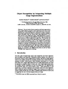
(c) Object 2
D. Results Experiments were performed using the cubes in Figure 2. In the first experiment we used cube 1 and cube 2. The two cubes yield different observations from orientation 1 and 2, but in orientations 3 and 4 the observations are the same. The robot should be able to identify correctly the cubes after performing an observe action in states s11 , s12 , s21 and s22 . However, when it is facing the object from orientation 3 or 4, the robot is not able to identify directly the object. Furthermore, the robot should have different behaviors in both orientations. While at orientation 3, the shortest way to identify the objects is to go to orientation 2 where objects can be desambiguated, in orientation 4 it should choose to go to orientation 1. The actions that the robot needs to perform in order to minimize the cost of identification are different. In the first case it should chose to rotate right (moving from states s∗,3 to s∗,2 ) and in the second case it should chose to rotate left (moving from states s∗,4 to s∗,1 ). In table I, we show the policy chosen by the robot, when facing each of the orientations of cube 2. Note that the policies described match what was just described. In our second experiment, which is exemplified in table II, we used the first and the third cube. The two cubes differ only in one face, but have two identical faces from the point of
(d) Object 3 Fig. 2. Objects used in the experiments. The objects have in total 6 different faces. The first object has 2 identical faces, o1 , plus 2 different ones, o2 , o3 . The second object shares two faces with object 1: o1 and o3 and has 2 new faces o4 and o5 . The third one is identical to the first, but only one face changed, o6 . The views represented do not correspond to any observation obtained from the robot and are indented solelly for describing the objects. In particular the viewpoints used were chosen to highlight the differences and similarities between objects.
view of the observations, i.e., the color histograms retrieved from orientations 2 and 4 are exactly the same. From the point of view of recognition, there is one single orientation, s∗,1 , which allows the robot to differentiate the two objects. From all the other states, the robot will have to rotate with relation to the object in order to arive at that specific state. All the observations that it may do in any other state will not help the robot in the recognition task. In the example in table II this is reflected in the policies presented for the
initial states s∗,1 , s∗,2 and s∗,3 . We also note that, due to the ambiguity in observations from state s∗,2 and s∗,4 in both cubes, if the robot starts in one of these states the policy will not be optimal in the sense that it produces more movements than those strictly required to disambiguate between objects. After the first observation, the belief state is the same for both states s∗,2 and s∗,4 and thus the policy will dictate the same action in both cases. While in one of the cases, this action may lead the robot directly to the state where it disambiguate the objects, s∗,1 , in the second state, the same action will take him to state s∗,3 . Initial State s2,1
Initial Image
Initial State s2,1
Initial Image
Actions observe identif y2
s2,2 observe rotateRight observe identif y2 s2,3 observe rotateRight rotateRight observe identif y2
Actions observe identif y2 s2,4
observe rotateRight observe rotateRight rotateRight identif y2
s2,2 observe identif y2 TABLE II P OLICY FOR EXPERIMENT 2
s2,3 observe rotateRight observe identif y2
s2,4 observe rotateLeft observe identif y2 TABLE I S ET OF ACTIONS PERFORMED BY THE ROBOT DURING EXPERIMENT 1, CONSIDERING THAT IT STARTS IN EACH OF THE I NITIAL S TATES .
V. C ONCLUSIONS AND FUTURE WORK In this work, we showed how to formalize an active object recognition task as solving an offline POMDP and provided evidence, through simulation, that the policies obtained performed observations only from the viewpoints which provided direct disambiguation between states. The main relevance of our result is that we did not formulate the problem in terms of the commonly used information theory. Instead, we formulated the problem solely in terms of control costs. The policies, obtained by solving our POMDP problem, still ensure that the robot always chooses the observations that provide most information. The robot only performs observations which actually contribute to a decrease on the uncertainty in the current state. By formulating the problem uniquely in terms of control costs, we can provide the robot with an a priori policy. There is no need to re-solve the POMDP during run-time and the
robot does not incur in the heavy time penality caused by the extra computational effort. As future work, it is important to study the impact of adding multiple objects in the POMDP formulation. Adding more objects leads to occlusions other than self occlusion which are more difficult to model offline. ACKNOWLEDGMENT This work was partially supported by the Carnegie Mellon/Portugal Program managed by ICTI from Fundac¸a˜ o para a Ciˆencia e Tecnologia. Susana Brand˜ao holds a fellowship from the Carnegie Mellon/Portugal Program, and she is with the Institute for Systems and Robotics (ISR), Instituto Superior T´ecnico (IST), Lisbon, Portugal, and with the Department of Electrical and Computer Engineering, Carnegie Mellon University, Pittsburgh, PA. The views and conclusions of this work are those of the authors only. R EFERENCES [1] S. Chen, Y. F. Li, J. Zhang, and W. Wang, Active Sensor Planning for Multiview Vision Tasks, 1st ed. Springer Publishing Company, Incorporated, 2008. [2] H. Borotschnig, L. Paletta, M. Prantl, and A. Pinz, Appearance-based active object recognition, Image and Vision Computing, vol. 18, 2000. [3] J. Denzler and C. M. Brown, it Information theoretic sensor data selection for active object recognition and state estimation, IEEE Trans. Pattern Anal. Mach. Intell., vol. 24, pp. 145157, February 2002. [4] R. Eidenberger and J. Scharinger, Active perception and scene modeling by planning with probabilistic 6d object poses, in Intelligent Robots and Systems (IROS), 2010 IEEE/RSJ International Conference on, 2010, pp. 1036 1043. [5] M. T. J. Spaan and N. Vlassis, Perseus: Randomized point-based value iteration for POMDPs, Journal of Articial Intelligence Research, vol. 24, pp. 195220, 2005.