object categorization in which the robot uses the natural sounds produced by objects .... The experiments in this paper use the dataset and sound representation ...
From Acoustic Object Recognition to Object Categorization by a Humanoid Robot Jivko Sinapov and Alexander Stoytchev Developmental Robotics Laboratory Iowa State University {jsinapov, alexs}@iastate.edu Abstract— Human beings have the remarkable ability to categorize everyday objects based on their physical and functional properties. Studies in developmental psychology have shown that infants can form such object categories by actively interacting and playing with objects in their surroundings. It is infeasible to pre-program a robot with knowledge about every single object that might appear in a home or an office. If robots are to succeed in human inhabited environments, they would also need the ability to form object categories and relate them to one another. In this work, we present an approach to interactive object categorization in which the robot uses the natural sounds produced by objects to form object categories. The method is evaluated on an upper-torso humanoid robot which performs five different manipulation behaviors (grasp, shake, drop, push, and tap) on 36 common household objects (e.g., cups, balls, boxes, pop cans, etc.). Using unsupervised hierarchical clustering, the robot is able to form a hierarchical taxonomy of the objects that it interacts with. The results show that the formed categories capture certain physical properties of the objects and allow the robot to quickly recognize the correct category for a novel object after a single interaction with it.
I. I NTRODUCTION According to psychologist Don Norman, natural sound conveys valuable information about the things we cannot see [1]. Natural sound also contains information about the interaction between the physical objects that generate it [1, p. 103]. Studies in psychology and cognitive science have shown that humans can extract the physical properties of objects from the sounds that the objects produce [2, 3]. Unlike our sense of vision, which is always constrained to a particular viewing direction, our auditory sense allows us to infer events in the world that are often outside the reach or range of other sensory modalities [1, p. 103]. A robot operating in a human-inhabited environment should be able to use sound as a source of information about events in its immediate surroundings. For example, such a robot could use sound to recognize important events in the home or office (e.g., an object falling to the ground) without the need for a direct line of sight. Like humans, humanoid robots will undoubtedly interact with objects (whether purposefully or by accident) outside of their field of view - in which case auditory input may be the primary source of information about the nature of the object. This work addresses the problem of how a robot can use acoustic information to learn about common household and office objects and their physical properties. Inspired by
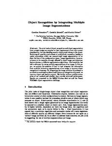
a) September 2008
b) April 2009
Fig. 1. The humanoid robot used in the experiments. a) the robot at the time the experiments were conducted; b) the robot in its current form.
principles and insights from developmental psychology, we present a framework in which the robot learns about natural sounds of physical objects through its own active interaction with them. Several key issues are addressed: •
• •
Can a robot learn to recognize a large set of objects using only acoustic information? Can a robot form object categories using natural sound? Do these learned object categories capture some of the physical properties (e.g., material type) of the objects?
To investigate these questions, we used a humanoid robot (see Figure 1) which interacts with 36 common objects by performing five different behaviors on them: grasping, shaking, dropping, pushing, and tapping. The robot represents each detected sound as a sequence of state activation patterns through a Self-Organizing Map (SOM). The SOM allows the robot to turn the high-dimensional sound input into a sequence of tokens from a finite alphabet (i.e., the set of nodes in the map). Using supervised learning methods, the robot is able to learn models that can perform object recognition using sound alone, as well as detect certain physical properties of the object (e.g., material type). Furthermore, using an unsupervised approach, the robot is able to form a hierarchical object categorization (i.e., a taxonomy) of the objects it explored, which captures some of their physical properties.
II. R ELATED W ORK A. Psychology The work presented in this paper is directly inspired and motivated by studies and research in psychology and cognitive science. In particular, the ecological approach to auditory perception provides the insight that everyday listening consists of perceiving the properties of a sound’s source (e.g., a car engine, footsteps, etc.), rather than the properties of a sound itself (e.g., pitch, tone, etc.) [2]. Hence, everyday listening is an important source of information - it allows us to perceive events outside our field of view, as well as recognize the physical properties of the objects involved. These insights have been confirmed by numerous experimental studies involving human subjects. For example, Warren et al. [4] demonstrate that humans are extremely good at categorizing individual sound tokens extracted from bouncing and breaking acoustic events. Furthermore, sound also allows us to perceive certain physical properties of objects: Grassi et al. [3] show that human subjects were able to provide reasonably good estimates for the size of a ball dropped on plates by simply hearing the impact sound. Giordano et al. [5] conducted a study which demonstrated that human beings can accurately recognize an object’s material (one of wood, glass, steel and plexiglass) when listening to the sounds generated when the object is struck. Motivated by these examples, the work in this paper investigates methods that would allow a robot to use sound as a source of information about objects in a similar manner. B. Robotics Despite the importance of natural sound, there have been relatively few studies examining how a robot can use sound as a source of information about objects, and their physical properties. One of the first studies that explore this topic was conducted by Krotkov et al. [6] in which the robot identifies the material type (aluminum, brass, glass, wood, and plastic) of several objects by probing them with its end effector. In a similar fashion, Richmond et al. [7] [8] have developed a robot platform for measuring contact sounds between a robot’s end-effector and objects of different materials. By modeling the spectrogram of the sounds using spectrogram averaging across multiple trials, the robot was able to detect different types of materials from contact sounds. Torres-Jara et al. [9] demonstrated a robot that can recognize objects using the sounds generated when tapping on them with its end effector. After tapping on a novel object, the spectrogram of the detected sound is matched to one that is already in the training set which results in a prediction for the object’s type. This allowed the robot to correctly recognize four different objects.
Object Material Contents
Object
Material Contents
paper
no
wood
no
paper
no
wood
no
paper
yes
wood
no
metal
no
plastic
yes
metal
no
plastic
yes
metal
no
metal
no
plastic
no
other
no
plastic
no
plastic
yes
plastic
no
paper
yes
plastic
no
plastic
no
other
no
plastic
yes
paper
no
plastic
no
plastic
no
metal
no
plastic
no
plastic
no
paper
no
metal
no
plastic
no
other
no
plastic
yes
plastic
no
plastic
yes
plastic
yes
Fig. 2. The 36 objects used in the experiments (not shown to scale). First column, from top to bottom: pasta box, paper cup, box of paperclips, metal cup, metal plate, metal flange, hockey puck, plastic green cup, plastic green ball, hard plastic bottle, styrofoam eraser, egg carton, detergent bottle, soft plastic bottle, empty cracker box, cosmetic bottle, coffee jar, small pill bottle; Second column: wooden stick, wooden plank, wooden cube, vitamin C bottle, tupperware (with play block inside), metal box, tennis ball, box of thumbtacks, box of spoons, empty shampoo bottle, box of screws, plastic container, pop can (Red Bull), pink plastic cup, pop can (Mt. Dew), rubber ball, orange plastic ball, mixed nuts jar.
III. E XPERIMENTAL S ETUP
After
Drop
Shake
Grasp
Before
Push
These previous studies, however, involved a relatively small number of objects and exploratory robot behaviors. In our previous work [10] we have shown that sound-based object recognition can be scaled up to a larger number of objects across multiple behaviors. Our robot used three machine learning methods (k-Nearest Neighbor, Support Vector Machine and Bayesian Network) to perform object recognition on eighteen different objects by applying three different behaviors (push, grasp, and drop). Features extracted from the spectrogram of each sound were used as input to the robot’s recognition model. The study in [10] was expanded in [11] to include an even larger number of objects (36) and two new behaviors tapping and shaking. The robot was able to recognize the type of object and the type of interaction (i.e., behavior) using only the detected sound, and the sound feature representation was shown to be superior to that of [10]. The experiments in this paper use the dataset and sound representation proposed in [11] to show how a robot can not only perform acoustic-based object recognition, but also form object categories and detect the physical properties of objects from natural sound.
The robot used in this study is an upper-torso humanoid robot, with the 7-DOF Barrett Whole Arm Manipulator (WAM) and the 3-finger Barrett Hand as its end effector (see Fig. 1.a). The robot arm is controlled in real time from a Linux PC at 500 Hz over a CAN bus interface. The robot is equipped with a Rode NT1-A microphone, also seen in Fig. 1.a. Sound input was recorded at 44.1 KHz using the Java Sound API over a single 16 bit channel. The microphone’s output was routed through an ART Tube MP Studio pre-amplifier. B. Objects The set of objects, O, that the robot interacts with consists of 36 different objects, shown in Fig. 2. The objects include common household items such as balls, cups, containers, bottles, boxes, etc. Some of the objects (e.g., the coffee jar, the box of thumbtacks, etc.) have contents inside of them which produce sounds when shaken. The objects are made of varying materials including metal, plastic, rubber, paper, and wood. The selection criteria for the objects were: must be graspable by the robot, must not contain liquids (even if they could), and must not be fragile (i.e., no glass objects). Each object was manually labeled with two labels corresponding to two different object properties: 1) the object’s material type (out of five possible categories); and 2) whether or not the object has contents inside of it (either yes or no). In the case of the material property, several different materials were considered: metal, wood, plastic, and paper. Objects with unique materials were put in the category of other. It is important to note that the labeling, even though performed by a human, should be considered noisy since some objects contain more than one material. Furthermore, while only 5 material
Tap
A. Robot
Fig. 3.
Before and after snapshots of the five behaviors used by the robot.
categories were considered, the actual number of materials present is much higher - for example, the plastic used to make the plastic bottle is quite different from the plastic used to make the plastic ball. C. Behaviors The robot’s set of behaviors, B, consists of five exploratory behaviors that the robot performs on each object: grasp, shake, drop, push, and tap. The behaviors were implemented using the Barrett WAM API. Fig. 3 shows before and after images for each exploratory behavior. The recording of each sound was automatically initiated at the start of each behavior and stopped once the behavior was completed. IV. LEARNING METHODOLOGY A. Feature Extraction using a Self-Organizing Map The robot in this study employs the sound feature representation introduced in [11], repeated here for clarity. Each sound, Si , is represented as a sequence of nodes in a Self-Organizing Map (SOM) [12]. To obtain such a representation, features from each sound were first extracted using the log-normalized Discrete Fourier Transform (DFT). The DFT was computed
0.1
0.05
a)
0
−0.05
−0.1
0
1
2
3
4
5
6
7 4
? Sphinx4
x 10
? 5
10
b)
15
20
25
30
50
100
150
200
250
300
350
400
450
? Trained SOM ? c)
Si :
si1
si2
si3
...
sili
Fig. 4. Audio signal processing and sound representation: a) The raw sound recorded after the robot performs the shake behavior on the Vitamin C bottle. b) Computed spectrogram of the sound. The horizontal axis denotes time, while the vertical dimension denotes the 33 frequency bins. Orange-yellow color indicates high intensity. c) The sequence of states in the SOM for the detected sound, obtained after each column vector of the spectrogram is mapped to a node in the SOM. The length of the sequence Si is li , which is the same as the length of the horizontal time dimension of the spectrogram shown in b). Each sequence token sij ∈ A, where A is the set of SOM nodes. Figure adapted from [11].
parameters for a non-growing 2-D single layer map. Figure 5 gives a visual overview of the training procedure. After training the SOM, each spectrogram, Pi , is mapped to a sequence of states, Si , in the SOM by mapping the columns of Pi to nodes in the map. To do this, each column spectrogram vector cij ∈ R33 is mapped to the node in the SOM with the highest activation value given the input cij . Thus, each sound is represented as a sequence, Si = si1 si2 . . . sili , where each sik ∈ A, A is the set of SOM nodes, and li is the number of column vectors in the spectrogram, as shown in Fig. 4. In other words, each sequence Si consists of a sequence of activated states in the SOM. The machine learning algorithm used in this study requires a symmetric similarity function that can compute how similar two sequences Si and Sj are. Computing similarity measures between a pair of sequences over a finite alphabet (e.g., strings) is a well established area of computer science, resulting in a wide variety of algorithms for exact and approximate string matching [15]. In this study, we define a similarity function, N W (Si , Sj ), between two such sequences to be the normalized global alignment score using the NeedlemanWunch alignment algorithm [16, 15]. The global sequence alignment algorithm has been used for string comparison in various domains, such as bioinformatics, and natural language processing, among others [15]. To compute the score between two sequences, a substitution cost must be defined over each pair of tokens in the alphabet. In this study, the substitution cost between two states sp and sq is set to the Euclidean distance between the corresponding SOM nodes (each of which is described by its x and y coordinate in the 2-D plane) in the map. B. Data Collection
using 25 + 1 = 33 frequency bins with a window of 26.6 milliseconds (ms), computed every 10.0 ms. The SPHINX4 natural language processing library (with default parameters) was used to compute the DFT [13]. Fig. 4 a) and b) show an sample sound wave and the resulting spectrogram after applying the Fourier transform. The spectrogram encodes the intensity level of each frequency bin (vertical axis) at each given point in time (horizontal axis). Let Pi be a spectrogram, such that Pi = [ci1 , ci2 , . . . , cili ] where each cij ∈ R33 (i.e., cij is the 33-dimensional column feature vector of the spectrogram at time slice j) and li is the number of column vectors in the spectrogram Pi . Given a collection of spectrograms, P = {Pi }K i=1 , a set of column vectors is sampled from them as an input dataset used to train a two dimensional SOM of size 6 by 6, i.e., containing a total of 36 nodes. The SOM is trained with input data points, cji ∈ R33 which represent the intensity levels for each of the 33 spectrogram frequency bins at a given point in time. Due to memory and runtime constraints, only 1/8 of the total available column vectors in P, sampled at random, were used to train the SOM. The SOM was trained using the Growing Hierarchical SOM toolbox for Java [14]. The default
Let B = [grasp, shake, drop, push, tap] be the robot’s set of exploratory behaviors. The robot performs 10 trials with each of the 36 objects for each of the 5 behaviors, resulting in a total of 5 × 10 × 36 = 1800 interactions. During the ith trial, the robot records a data triple of the form (Bi , Oi , Si ), where Bi ∈ B is the performed behavior, Oi ∈ O is the object in the interaction, and Si = si1 si2 . . . sili is the sequence of activated SOM nodes over the duration of the sound. In other words, each triple, (Bi , Oi , Si ), indicates that sound Si was detected when performing behavior Bi on object Oi . C. Learning Algorithm The first task of the robot is to learn a model such that given a sound sequence, Si , the robot can estimate the object class, Oi , present in the interaction that generated the sound Si . In other words, given a sound Si , the robot should be able to estimate P r(Oi = o|Si ) for each object o ∈ O. To estimate these probabilities the robot uses the k-Nearest Neighbor machine learning algorithm. K-Nearest Neighbor (kNN) is a memory-based learning algorithm which does not build an explicit model of the data. Instead, it stores all labeled training data points and uses them when the model is queried to make a prediction [17, 18].
Column Vectors:
-
... ..
.
Predicted:
Actual
Set of Spectrograms:
40
4
0
0
6
42
0
0
0
0
21
6
0
0
8
35
Trained SOM: ? �
GHSOM Toolbox
similar
different
similar
different
Fig. 5. Illustration of the procedure used to train the Self-Organizing Map (SOM). Given a set of spectrograms, a set of column vectors are sampled at random and used as a dataset for training the SOM. Figure adapted from [11]
When making a prediction on a test data point, k-NN finds its k closest neighbors in the training set, i.e., given a test data point Si , k-NN finds the k training data points most similar to Si . The algorithm returns a class label prediction which is a smoothed average of the labels of the selected neighbors. As in our previous work [11], the normalized global alignment score, N W (Si , Sj ), is used as the similarity metric between two data points Si and Sj . In the experiments in this study, k was set to 3. An estimate for P r(Oi = o|Si ) is computed by counting the class labels of the k neighbors. For instances, if two of the three neighbors have object class label plastic ball then P r(Oi = plastic ball|Si ) = 23 . Similarly, if the class label of the remaining neighbor is plastic cup, then P r(Oi = plastic cup|Si ) = 13 . V. O BJECT C ATEGORIZATION In this study, the robot uses its object recognition model to acquire object categories using an unsupervised hierarchical clustering approach. The intuition behind the method used by the robot is that if a set of objects make very similar sounds, it will be difficult for the robot to detect which precise object from the set was present during the interaction. For example, it may be the case that the robot’s recognition model outputs rubber ball in many of the cases when the actual object in the interaction is tennis ball. In such a scenario, the two objects should be considered similar and hence, grouped into a category (see Figure 6). Following, we show how: 1) the robot uses its recognition model to construct a pairwise object similarity matrix; and 2) how given such a similarity matrix, the robot constructs a hierarchical clustering of the objects.
Fig. 6. A simple example of how a confusion matrix can be used as a way to measure object similarity. The ij th entry in the confusion matrix specifies how often the sound generated by object i was classified as being generated by object j (out of 50 possible trials, 10 for each of the 5 behaviors). For example, the robot’s recognition model outputs rubber ball in several of the trials in which the actual object in the interaction is tennis ball. Similarly, the robot also confuses the two pill bottles with each other, and hence, they should be considered similar in terms of the sounds they generate. Section V describes how the confusion matrix is used to compute a symmetric pair-wise similarity measure between each pair of objects, which in turn is used as an input to a hierarchical clustering algorithm.
A. Object Similarity Matrix To compute an object similarity matrix, the robot uses the k-NN object recognition model (described in the previous section) as follows. Let D = {(Bi , Oi , Si )}N i=1 be the set of trial data available to the robot. Next, the robot evaluates its own object recognition model by performing 10-fold crossvalidation on the available data. The result of this procedure is a |O| × |O| confusion matrix C, where the value in the entry Cij indicates how often object i was predicted as object j. To construct a symmetric similarity matrix between each pair of objects, let the matrix C′ be defined such that each ′ entry Cij = 0.5 ∗ Cij + 0.5 ∗ Cji . Finally, the values in the resulting matrix are scaled so that each entry is in the range between 0.0 and 1.0, and the diagonal values are set to 1.0. The result of this procedure is a symmetric similarity matrix W. Figure 6 visualizes how a confusion matrix can be used as a way to detect pair-wise object similarity. The next subsection describes how the resulting similarity matrix W is used as input to a hierarchical clustering algorithm.
#1
#2
#3
#4
#5
#6
#7
#8
#9
Fig. 7. Visualization of the learned hierarchical object categorization, obtained after recursively applying the Spectral Clustering algorithm using the acquired object similarity matrix. The similarity matrix was obtained from the confusion matrix after the robot’s k-NN object recognition model was evaluated using 10-fold cross-validation. Nine object categories are learned, many of which group objects either by their material type, or by whether or not the objects have contents inside of them.
B. Hierarchical Clustering To construct an hierarchical object categorization, the robot uses the Spectral Clustering algorithm which falls into the family of graph-based or similarity-based clustering algorithms [19]. Given a similarity matrix, W, the algorithm partitions the input data points (i.e., the objects) into disjoint clusters by exploiting the eigenstructure of the matrix W. Because finding an optimal graph partitioning is NP-complete, Shi and Malik [20] proposed an approximation that optimizes the normalized cut objective function. The algorithm, as applied to our problem, can be summarized in the following steps: 1) Let Wn×n be the symmetric matrix containing the similarity score for each pair of objects. 2) Let Dn×n be the degreePmatrix of W, i.e., a diagonal matrix such that Dii = j Wij . 3) Solve the eigenvalue system (D − W)x = λDx for the eigenvector corresponding to the second smallest eigenvalue and use it to bi-partition the graph. 4) If necessary, recursively bi-partition each subgraph obtained at Step 3. Hence, the algorithm recursively bi-partitions the graph (which is induced by the similarity matrix W) until a stopping
criterion in reached, producing a tree structure. In this study, the algorithm is recursively applied until the size of each subgraph falls down to 5 or less objects (the number was chosen heuristically based on the input size (36 objects) such that each object category will consist of at least 3 objects). The output of this procedure is a hierarchical taxonomy (i.e., a tree), T , which specifies the learned hierarchical object categorization. VI. R ESULTS A. Learned Object Categories Figure 7 shows the learned hierarchical object categorization after obtaining the similarity matrix and recursively applying spectral clustering. At first glance, some of the categories appear to capture certain physical properties of the objects: for example, clusters 1 and 2 (which are siblings in the tree T ) consist almost exclusively of metal objects. Cluster 3, on the other hand contains five of the objects that have small contents inside of them (e.g., pill bottles and boxes of thumbtacks, screws, and paperclips). Cluster 4 contains three out of the four balls in the dataset. All except one of the paper objects in the set are grouped together in Cluster 5. As expected, the two plastic cups (which differ only in size) are grouped together, along with a plastic shampoo bottle in Cluster 6.
TABLE I I NFORMATION G AIN I NDUCED BY THE L EARNED O BJECT
TABLE II R ECOGNITION ACCURACY WITH K -NN MODEL
C ATEGORIZATION WITH RESPECT TO TWO PHYSICAL PROPERTIES Behavior Object property
Entropy at root
Avg. leaf entropy (learned)
Avg. leaf entropy (random)
Material Contents
1.40 0.56
0.42 ± 0.32 0.18 ± 0.27
0.86 ± 0.25 0.40 ± 0.29
Cluster 7 contains mostly wooden objects, while Cluster 8 contains exclusively plastic objects. The last one, Cluster 9, appears to simply hold the remaining 4 objects, which vary by material (three plastic and one metal) and contents (the plastic tupperware has contents, while the rest do not). It is still desirable, however, to have a quantitative measure that captures the quality of the learned object taxonomy. To do that, we look at how well the taxonomy captures two physical properties of the objects: 1) their material, and 2) whether or not they have contents inside them. Following, each object is manually given a label corresponding to one of five material classes: plastic, paper, wood, metal, and other (Figure 2 shows how each object was labeled). Given a set of objects O′ (which may be a sub-set of the full set O), let pi for i = 1, . . . , n be the estimated probability that an object drawn from P that set will be made of the ith material n ′ type. Let Hn = − i=1 pi log2 (pi ) be the Shannon entropy ′ for the set O . If the learned categorization T captures the physical property of material, then the average entropy for the objects in each leaf node in T should be significantly lower than the entropy at the root node. In other words, the taxonomy will induce an information gain with respect to the physical property of material. Similarly, the taxonomy should induce such an information gain with respect to the second physical property we examine, which is whether or not an object has contents inside of it. Naturally, some information gain will be the result of the fact that the leaf nodes will contain significantly less objects than the root node. To control for this, the entropies at the leaf nodes are also computed for a random object categorization, obtained by randomly permuting the similarity matrix W used to compute the hierarchical clustering. This procedure was repeated 10 times, in order to compute robust estimates for the mean leaf entropy and its standard deviation. In the case of the learned object categorization, the mean and standard deviations were estimated from the nine leaf nodes in the learned taxonomy. The results of this test are summarized in Table I. As expected, there is substantial information gain induced by the learned categorization with respect to the two physical properties considered. More importantly, the information gain of the learned object taxonomy is greater than that of a random object categorization. This result shows that object categorization using acoustics can capture some of the physical properties of the objects that the robot is exposed to.
Grasp Shake Drop Push Tap Average
Object Recognition 67.89 49.47 85.79 82.89 78.15 72.84
% % % % % %
Category Recognition 81.94 60.00 94.44 93.06 87.22 83.33
% % % % % %
B. Object Category Recognition Next, the robot’s k-NN model is evaluated on how well it can detect the object in each interaction from the detected sound. Similarly, the robot is also evaluated on how well it can recognize the test object’s category (i.e., which leaf node in the learned taxonomy T does the object belong to). The performance of the models is reported in terms of the percentage of correct predictions (i.e., accuracy) where: % Accuracy =
# correct predictions # total predictions
× 100
The accuracies in both cases are estimated using 10-fold cross validation. The results are summarized in Table II. As a reference, the expected change accuracy for object recognition is 1/36 ≈ 2.7%. The robot is best able to recognize the object in the drop, push, and tap interactions. However, even when shaking the objects, the robot is able to achieve recognition accuracy substantially better than chance since many of the objects have distinct contents inside of them which make noise when shaken. The results also show that the robot achieves high recognition accuracy when predicting the category of the object as opposed to the object itself. On average, there is a ≈ 10% improvement over the object recognition accuracy. This result indicates that even when the robot is unable to recognize the precise object in the interaction, it can still detect the category of that object with high accuracy. C. Detecting the Physical Properties of Objects In this experiment, the task of the robot is to detect two physical properties of the object from the sound that it generates. The two properties are: 1) the object’s material type (5 class classification problem), and 2) whether or not the object has contents inside of it (binary classification problem). This experiment tests how well the robot can perform acoustic recognition when the objects’ labels are provided externally (i.e., by a human), as opposed to the robot’s own object categorization. This experiment is inspired by studies in psychology [3], which show that human beings can often perceive certain physical properties of the objects (such as size and material) from the sound that the objects generate during physical interactions. As in the previous experiment, the performance accuracies are estimated using 10-fold crossvalidation. Table III shows the results of this experiment. For reference, the chance recognition accuracies for the two physical prop-
TABLE III R ECOGNITION OF P HYSICAL P ROPERTIES WITH K-NN MODEL Behavior Grasp Shake Drop Push Tap Average
Material (five classes) 84.17 59.17 92.50 94.17 90.28 84.06
% % % % % %
Contents (yes/no) 91.38 95.55 98.61 97.22 96.11 95.78
% % % % % %
erties are 52.78 % and 75.00 % respectively for the object’s material type and contents (the chance rates are obtained by labelling each test data point with a class label sampled from the prior class distribution). The results indicate that the robot is able to recognize the material of the test object, as well as whether the object has contents inside of it substantially better than chance. The material of the objects is most easily detected when they are dropped or pushed. It is important to note that while only 5 material classes were considered, the actual number of materials present in the selected objects is much higher. For example, there are objects with diffierent types of plastic (e.g., soft plastic bottle vs. hard plastic ball) and different types of paper (egg-carton vs. pasta box vs. styrofoam eraser). Yet, the robot is able to achieve a reasonably high recognition accuracy. These results confirm that natural sound contains invariant information regarding the physical properties of objects. VII. C ONCLUSIONS AND F UTURE W ORK This paper described how a robot can couple exploratory behaviors on objects with the natural sounds produced during these interactions in order to accurately recognize and categorize different household objects. The robot used its acousticbased recognition model to detect pair-wise object similarity, allowing it to construct a full hierarchical object categorization in an unsupervised manner. The learned object categorization was quantitatively shown to capture two physical object properties: 1) the object’s material type, and 2) whether or not the object has contents inside of it. Finally, we showed that the robot can detect these two object properties using acoustics alone. Hence natural sound has an important role to play in the robot’s grounded representation of physical object properties. The robot represented sound input through the use of a SelfOrganizing Map, which helped reduce the dimensionality of each sound. The robot was evaluated on 36 different household objects, using 5 different exploratory behaviors: grasp, shake, drop, push, and tap. The number of objects and behaviors show that acoustic recognition can be scaled up to a large set of objects, across multiple different exploratory behaviors. The work presented here demonstrated some initial steps that allow a robot to learn about natural sound through its own interaction with the world. However, several key questions remain: how can a robot use its acquired models of natural sound to recognize interactions performed by others (e.g., humans)? How can the proposed acoustic-based object representation be
generalized to include sensory input across multiple modalities (e.g., vision, proprioception, etc.)? For future work, we plan to evaluate how well the robot can use its learned representation to reason about not only its own interactions with objects, but also those of others. A household robot that can detect an object breaking from across the hall will be far more useful than one that can only detect such an event through a direct line of sight. Furthermore, the proposed representation should be integrated with multiple modalities. For example, the sound of an object being dropped on the floor not only contains information about the event and the object, but also about the object’s actual movement (i.e., falling down). Extending the object categorization method to multiple modalities and interactions will allow a robot to learn precisely such audio-visual associations. R EFERENCES [1] D. Norman, The Design of Everyday Things. Doubleday, 1988. [2] W. W. Gaver, “What in the world do we hear? An ecological approach to auditory event perception,” Ecological Psychology, vol. 5, pp. 1–29, 1993. [3] M. Grassi, “Do we hear size or sound? Balls dropped on plates,” Perception and Psychophysics, vol. 67, no. 2, pp. 274–284, 2005. [4] W. Warren and R. Verbrugge, “Auditory perception of breaking and bouncing events: A case study in ecological acoustics,” Journal of Experimental Psychology: Human Perception and Performance, vol. 10, no. 5, pp. 704–712, 1984. [5] G. B. L. and M. S, “Material identification of real impact sounds: Effects of size variation in steel, glass, wood, and plexiglass plates,” Journal of the Acoustical Society of America, vol. 119, no. 2, pp. 1171–81, 2006. [6] E. Krotkov, R. Klatzky, and N. Zumel, “Robotic perception of material: Experiments with shape-invariant acoustic measures of material type,” in Experimental Robotics IV, ser. Lecture Notes in Control and Information Sciences. Springer Berlin/Heidelberg, 1996, vol. 223, pp. 204–211. [7] J. L. Richmond and D. K. Pai, “Active measurement of contact sounds,” in Proc. of the IEEE Conference on Robotics and Automation, 2000. [8] J. L. Richmond, “Automatic measurement and modelling of contact sounds,” Master’s thesis, University of British Columbia, 2000. [9] E. Torres-Jara, L. Natale, and P. Fitzpatrick, “Tapping into touch,” in Proc. of the Fifth International Workshop on Epigenetic Robotics, 2005. [10] J. Sinapov, M. Weimer, and A. Stoytchev, “Interactive learning of the acoustic properties of objects by a robot,” in Procceedings of the RSS Workshop on Robot Manipulation: Intelligence in Human Environments, Zurich, Switzerland, 2008. [11] ——, “Interactive learning of the acoustic properties of household objects,” in Procceedings of the IEEE International Conference on Robotics and Automation (ICRA), 2009. [12] T. Kohonen, Self-Organizing Maps. Springer, 2001. [13] K. E. Lee, H. W. Hon, and R. Reddy, “An overview of the SPHINX speech recognition system,” IEEE Transactions on Acoustics, Speech, and Signal Processing, vol. 38, no. 1, pp. 35–45, 1990. [14] A. Chan and E. Pampalk, “Growing hierarchical self organizing map (ghsom) toolbox: visualizations and enhancements,” in Procceedings of the 9th International Conference on Neural Information Processing (NIPS), 2002, pp. 2537–2541. [15] G. Navarro, “A guided tour to approximate string matching,” ACM Computing Surveys, vol. 33, no. 1, pp. 31–88, 2001. [16] S. Needleman and C. Wunsch, “A general method applicable to the search for similarities in the amino acid sequence of two proteins,” J. Mol. Biol., vol. 48, no. 3, pp. 443–453, 1970. [17] W. D. Aha, D. Kibler, and M. K. Albert, “Instance-based learning algorithm,” Machine Learning, vol. 6, pp. 37–66, 1991. [18] C. G. Atkeson, A. W. Moore, and S. Schaal, “Locally weighted learning,” Artificial Intelligence Review, vol. 11, no. 1-5, pp. 11–73, 1997. [19] U. von Luxburg, “A tutorial on spectral clustering,” Statistics and Computing, vol. 17, no. 4, pp. 395–416, 2007. [20] J. Shi and J. Malik, “Normalized cuts and image segmentation,” Pattern Analysis and Machine Intelligence, vol. 22, no. 8, pp. 888–905, 2000.