Active Shape Model with Inter-profile Modeling Paradigm for Cardiac Right Ventricle Segmentation Mohammed S. ElBaz1,2 and Ahmed S. Fahmy1,3 1
Medical Imaging and Image processing Lab., Center for Informatics Science, Nile University, Cairo, Egypt 2 Division of Image Processing, Department of Radiology, Leiden University Medical Center, Leiden, The Netherlands 3 Systems and Biomedical Engineering Department, Cairo University, Cairo, Egypt
[email protected]
Abstract. In this work, a novel active shape model (ASM) paradigm is proposed to segment the right ventricle (RV) in cardiac magnetic resonance image sequences. The proposed paradigm includes modifications to two fundamental steps in the ASM algorithm. The first modification includes employing the 2DPrincipal Component Analysis (PCA) to capture the inter-profile relations among shape’s neighboring landmarks and then model the inter-profile variations between the training set. The second modification is based on using a multi-stage searching algorithm to find the best profile match based on the best maintained profile’s relations and thus the best shape fitting in an iterative manner. The developed methods are validated using a database of short axis cine bright blood MRI images for 30 subjects with total of 90 images. Our results show that the segmentation error can be reduced by about 0.4 mm and contour overlap increased by about 4% compared to the classical ASM technique with paired Student’s t-test indicates statistical significance to a high degree for our results. Furthermore, comparison with literature shows that the proposed method decreases the RV segmentation error significantly.
1
Introduction
Segmentation of the right ventricle (RV) has recently gained a lot of the clinical research focus. This is due to new findings that confirm the relationship between the RV function and a number of cardiac diseases such as heart failure, RV myocardial infarction, congenital heart disease and pulmonary hypertension [1,2]. Since manual segmentation of the RV borders throughout the cardiac cycle is tedious process and may suffer from personal bias, and inter-observer variations; accurate computer-aided segmentation methods are required. One of the increasingly popular and successful segmentation approaches is the Active Shape Model (ASM) introduced by Cootes et.al [3,4]. ASMs have been used for many segmentation tasks including medical images [3,4]. The classic ASM paradigm [4] represent the object of interest by a set of labeled points called landmarks, these landmarks define the shape of the object. The global statistics of the shape variation is then examined from number of examples in N. Ayache et al. (Eds.): MICCAI 2012, Part I, LNCS 7510, pp. 691–698, 2012. © Springer-Verlag Berlin Heidelberg 2012
692
M.S. ElBaz and A.S. Fahmy
the training dataset by applying the Principal Component Analysis (PCA) on the landmarks of the training shapes to model the ways in which the points of the shape tends to move together through the training set [4]. Then, the gray-level appearance model that describes the typical image structure around each landmark is modeled by sampling a grey-level profile around each landmark then applies PCA on the training shapes profiles to model the profile appearance of each landmark in the shape independently. Throughout the image search, starting from the mean shape and initial model pose parameters (landmarks position, rotation and scaling), shapes are fitted in an iterative manner by fitting the appearance model of each landmark separately i.e. using local search. The shortcoming of the classical ASM paradigm is that while it models the global statistics of the shape variations, it merely builds a separate graylevel appearance model for each landmark in the shape. That is, the appearance model does not include any global information about the relationships among the appearance profiles of the different landmarks. Furthermore, searching for the best profile fit for each landmark independently might cause the contour to stick to local minimum. In this work, we propose a novel appearance profile modeling paradigm to overcome these shortcomings. The proposed paradigm called inter-profile modeling in which for each shape in the training set, the appearance profiles are set in matrix form and the Two Dimensional Principal Component Analysis (2DPCA) [6] is applied to capture the inter-profile relations among the shape’s landmarks and then to model the inter-profile variations between the different training shapes. Compared with PCA, 2DPCA algorithm is more efficient to deal with the proposed 2D profile matrices, as 2DPCA works directly on the 2D matrices without pre-transformation to 1D vector as required by PCA. This yields that 2DPCA constructs much smaller covariance matrix compared with PCA which gives 2DPCA a significant computational advantage [6,7]. Additionally, 2DPCA preserves the 2D integral structure and the spatial information of the input 2D matrices as opposed to the PCA which breakup this 2D integral through the 2D matrix to 1D vector transformation. Additionally, Multi-stage searching algorithm is also proposed to employ the modeled inter-profile variation to find the best profile match.
2
Methodology
Following from the active shape model algorithm [4], we apply the same shape modeling step. Then, for the profile modeling step we use a new profile-modeling paradigm as follows: 2.1
Inter-profile Appearance Modeling
We define the Inter-profile modeling as the process of capturing the profile modes of variation by the ways in which all shape appearance profiles tend to change together through the training set. In order to achieve this modeling, we start by constructing a grey level appearance profiles matrix (shortly we will refer to it as profiles matrix) for each shape ( where similar to the ASM [4], each profile is perpendicular on the
Active Shape Model with Inter-profile Modeling Paradigm
693
contour and sampled with length of ns pixels on either side of the contour). The profiles matrix holds all shape profiles together. That is, given a training set of K shapes, M landmarks and intensity profile of length N at each landmark, then (i=1,2,…,K) is given by, , ,
. . . .
,
…, …, (1) …,
Each row (i.e. grey-level profile) is normalized by the maximum value in the row to compensate for the illumination differences. 2.2
Capturing the Inter-profile Variations Using 2D-PCA
In order to capture the modes-of-variations of the inter-profile matrices of the training database, two-dimensional PCA (2DPCA) is employed [7] with its two versions (horizontal and vertical) [8] to capture both the horizontal and vertical inter-profile variaand covariance tions. For the horizontal 2DPCA version, the mean profile matrix matrix Ct are computed as G
K
∑K G
(2)
and
C
K
∑K
G
G
T
G
G
(3)
is expressed by matrix ,Pgh, of The grey-level variation around the mean profile size N×D. That is Pgh contains the D eigenvectors of Ct corresponding to the D largest eigenvalues ʎ , ʎ , … , ʎ . The horizontal-based new profiles matrix approximation can be computed as G
G
P b
T
(4)
Contarary to the classical ASM vector model parameters, here, the model parameters are expressed by the matrix bgh of size D×M computed as b
P
T
G
G
T
(5)
Thus bgh captures the horizontal inter-profile relations between the landmarks profiles. We apply constraints to the parameter bgh to ensure plausible profiles (e.g. 3√ʎ ). To capture the grey-level modes of variation using the vertical 2DPCA, the same procedure discussed above is followed except that the input to the vertical 2DPCA is the transpose of the profiles matrix Gi. This yields a model defined by the matrices: Pgv and bgv. During the search for the object that best fits the constructed shape model; some goodness-of-fit measure is needed. In the proposed modeling paradigm, the inter-profile model is given by the matrices and Pgh (assuming horizontal 2DPCA). The parameters required to best fit the horizontal model to Gi is given by the matrix bgh computed by (5). To measure how well the model fits the
694
M.S. ElBaz and A.S. Fahmy
profiles matrix Gi, the Frobenius-norm of the parameter matrix bghis used as a distance measure. The Frobenius-norm, Fh, is given by, F
b
F
∑
,
b
x, y
(6)
It is worth noting that Fh tends to zero as the quality of fit improves. 2.3
Iterative Multi-stage Bidirectional 2DPCA-Based Best Profile Search Algorithm
We define the best profile match as the profile which together with all other profiles in the profiles matrix yields maximum matrix fit. That is, the best profile match (fit) includes all shape’s profiles information in the fitting procedure. Following the classical ASM procedure, starting from the mean shape, each landmark is moved along the direction perpendicular to the contour to, ns, different positions on either side, evaluating a total of 2ns+1 positions. However, to employ the 2DPCA- based interprofile modeled variations, we propose two stage searching algorithm to find the best profile fit. In the first stage, the target is to reach to a combination of candidate profiles which have good inter-profile relations with each other. So, we start by initializing the profile’s matrix by the mean profile’s matrix (i.e ). Then, for each landmark, the 2ns+1 candidate positions is evaluated, for each evaluation, all rows of G remain the same except the row corresponding to the current landmark which is replaced by the current profile under evaluation(i.e. this row is replaced 2ns+1 times) and the profile with minimum F is the best profile fit for this landmark. This process is repeated for each landmark and at each time , the matrix is re-initialized by . Here, we should note that even we replace only the landmark’s corresponding row in G at each time, the resultant profile after each landmark evaluation is the profile that increases the overall inter-profile relation among the matrix (shape) profiles because in the calculation of ,F, (Eqn.6) all profiles in the matrix are included in the evaluation. Profiles constraints are applied on bgh (or bgv in the vertical modeling case) (e.g. |bgh|< 3 λ) to ensure plausible profiles. The result of this stage is matrix that holds the resultant best profiles (e.g. first row in holds the profile that gave the minimum F during first landmark fitting). In the second stage, G is initialized by , then similar to the first stage, for each landmark ,we evaluate for the best fit out of 2ns+1 candidate profiles using minimum F as the best fit criterion. Contrary to the first stage, after each landmark fit, we update the corresponding row in G by the profile that gives the minimum F (so, not to reinitialize after each landmark evaluation). Then, the updated matrix G is used in the evaluation of the next landmark best fit. This ensures that each landmark update or fit is considering the best of other shape landmarks profiles leading to fitting the whole shape towards the shape that maintains the best inter-profile relations. The second stage is iterated predefined number of times until either convergence (e.g. stop when 90% or more of the best found pixel along the search profile is within the central 50 % of the profile length) or completing the number of predefined iterations. The same two stage procedure is applied in case of the vertical fitting. Furthermore, bidirectional fitting procedure is applied to maintain both the horizontal and vertical inter-profile variations.
Active Shape Model with Inter-profile Modeling Paradigm
695
That is, for each candidate position we compute both the horizontal (the two-stages) followed by vertical fitting and also, the vertical followed by the horizontal fitting. Then we admit the fitting with the smaller final F to be the best fit for the current landmark in the current iteration. Additionally, similar to the classical ASM algorithm we may build the aforementioned inter-profile models for multiple resolutions; this may improve the speed and the robustness of the algorithm.
3
Experimental Setup
The dataset used in this study is the York dataset of short axis cardiac MR images [8]; this dataset was constructed by studying 33 subjects to mainly evaluate the LV segmentation results. In our experiments we have excluded three subjects (5, 6 and 27) from the dataset due to their low signal to noise ratio, resulting in 30 subjects (image sets) for our experiments. In each image set, three end-diastolic, midventricular slices were selected for the total of 90 images of 256 X 256 pixels; pixel sizes: 1.1719–1.6406 mm. For all of the 90 images, RV is manually outlined to be used as ground truth for automatic segmentation performance validation. Initial pilot experiments were performed to find the best ASMs parameters, fixed settings were selected that yielded good performance. The same parameters are used for both the classical and the proposed ASM. Training images are used to build the right ventricle specific statistical shape model. The shape model was built with 119 landmarks (M=119) which were distributed equally over the model contour. The first 16 modes (eigenvectors) are retained describing 99% of shape variations of the training dataset. For the construction of the gray-level appearance models, the grey level profile length chosen to be 2 pixels on either side of the landmarks (N=5); 98% of the appearance variation is explained, that represented by the first 4 eigenvectors for the vertical 2DPCA, and by 53 to 74 eigenvectors for the horizontal 2DPCA which varies based on the resolution level and training shapes included in the current crossvalidation iteration. Furthermore, two resolution levels are used for modeling. To compare segmentation performance between the classical ASM and our proposed method, overlap measure and point to curve error measure (P2C) are used which calculated as follows: Overlap
TP
Ω
TP FP FN
(7)
where TP stands for the true positive, FP for false positive and FN for false negative, Ω=1 for perfect overlap and Ω=0 if there is no overlap at all. P2C C , C
N
∑N
d p ,p
(8)
Where Ca denoting the automatically resulted contour, Cm denoting the manual deliis a point on Ca , is a point on Cm and d(…) neated contour (ground truth), represents the Euclidean distance between two points, if P2C=0 then there is perfect match between the automatic and manual contours while P2C=1 means total mismatch. To test the proposed algorithm performance, rough good shape parameters
696
M.S. ElBaz and A.S. Fahmy
(position and orientation) initialization is manually determined which the same for both algorithms under comparison. Table 1. Overlap and P2C measure results of the Classical ASM and the proposed method
Classic ASM Our method
Overlap μ±σ 0.74 ± 0.11 0.78 ± 0.06
Overlap median 0.76 0.79
P2C μ ± σ (mm) 1.13 ± 0.79 0.73 ± 0.37
P2C Median (mm) 0.88 0.62
Table 2. Mean segmentation errors reported in the literature and for our method
Authors Mitchell 01 [9]
No. subj. 54
Lorenzo 04[10]
10
Grosgeorget 10[11] Lötjönen 04 [12]
%P 45
Slice no. 3 Mid
Error (mm) 2.46 ± 1.39a
100
3 Mid
2.26 ± 2.13
59
100
6–10 Mid
2.27 ± 2.02
25
100
4-5
2.37 ± 0.5c
Abi-Nahed 06 [13]
13
-
-
1.1b
Sun et al. 10[14]
40
75
8-12
1.19 ± 0.28
proposed method
30
93
3 Mid
0.73 ± 0.37
%P percentage of pathological subjects. a RMS error. b No standard deviation provided. c Surface to surface error measure.
4
Results
In order to avoid bias, segmentation performance is evaluated using 5-fold crossvalidation strategy, the original dataset (n=90 images) is partitioned into 5 subsets with 18 images for each subset. Of the 5 subsets, a single subset is retained as the validation set for testing the model, and the remaining 4 subsets are used as training data. The cross-validation process is then repeated 5 times. To show the performance of our method, all results are compared with the classical ASM-based RV Segmentation method. The mean contour overlap measure and P2C error measure results of the experiment are given in Table 1. Furthermore, Table 2 presents the Point to curve (P2C) errors of our method along with segmentation errors collected from the literature for the right ventricle segmentation. A paired Student’s t-test was carried out to determine the level of statistical significance between the proposed method and the classical ASM which resulted in high significance for the P2C with p < 7.68X10⁻¹⁰ and also for the overlap with p < 2.22X10⁻¹⁵. Figure 2 shows an example of our proposed method segmentation performance in comparison with the classical ASM.
Active Shape Model with Inter-profile Modeling Paradigm
(a)
(b)
697
(c)
Fig. 1. (a) initial contour, (b) classic ASM result (green contour is ground truth and the blue contour is the segmentation result, (c) proposed ASM paradigm result
5
Discussion and Conclusion
Our results show that the proposed ASM with inter-profile modeling paradigm is rather accurate relative to the classical ASM with P2C errors around 0.7 mm. Table 1 shows that ASM with inter-profile modeling method improves the segmentation overlap measure between the automatic segmentation and the manual segmentation by about 4% than the classical ASM method with high statistical significance of p< 2.22X10⁻¹⁵ using paired t-test. Meanwhile, it shows that our method minimized the P2C error by about 0.4 mm in comparison with the classical ASM P2C error with high statistical significance of p< 7.68X10⁻¹⁰ using paired t-test. In building the shape model, shapes were aligned for rotation and translation while no scaling was included in the alignment step. In addition, For measuring how well the model fits the profile matrix (Eqn. 6), we have tested many norm evaluation methods including L1norm,L2-norm , infinity- norm and frobenius-norm. However, the frobenius-norm has given the best results. It is worth noting that although the maximum number of allowed iteration for the second stage in the search algorithm was set to 6 in all our experiments, a value of only 3 or 4 was sufficient to achieve reasonable results. Table 2 shows that the performance of our ASM with inter-profile modeling method substantially outperforms the recently published literature results. Herein, we should note that many of the presented literature results were obtained using 3D segmentation algorithms [9,10, 12, 13, 14], whereas our approach is a 2D based method. Although, it is required to be cautious when trying to compare techniques that use different MRI sequences, different segmentation protocols and different error criteria; the high statistical significance of the proposed paradigm compared to the classical ASM and the difference between proposed method and other literature results should be encouraging. Matlab implementations for both the classical ASM and ASM with inter-profile modeling using 2.00 GHz Intel Core 2 Duo laptop are used to compare the speed of both algorithms. For the classical ASM, it required about 710 seconds for the segmentation of the whole 90 Images while for our method it required about 1015 seconds. The proposed method is relatively more computationally expensive than the classical ASM but this difference seems to be acceptable due to the significant improvement compared to the classical ASM. In conclusion, the new ASM with inter-profile
698
M.S. ElBaz and A.S. Fahmy
modeling paradigm introduced in this paper substantially improves the original ASM method performance and an effective method to segment the cardiac Right Ventricle. Acknowledgements. This work is supported in part by grant #1979 from the Science and Technology Development Fund (STDF), Egypt.
References 1. de Groote, P., Millaire, A., Foucher-Hossein, C., Nugue, O., Marchandise, X., Ducloux, G., et al.: Right ventricular ejection fraction is an independent predictor of survival in patients with moderate heart failure. J. Am. Coll. Cardiol. 32, 948–954 (1998) 2. Matthews, J.C., Dardas, T.F., Dorsch, M.P., Aaronson, K.D.: Right sided heart failure: diagnosis and treatment strategies. Curr. Treat. Options Cardiovasc. Med. 10, 329–341 (2008) 3. Cootes, T., Taylor, C.J., Cooper, D.H., Graham, J.: Active shape models – their training and application. CVIU 61(1), 38–59 (1995) 4. Cootes, T., Hill, A., Taylor, C., Haslam, J.: The use of active shape models for locating structures in medical images. Image Vis. Comput. 12, 355–366 (1994) 5. Sirovich, L., Kirby, M.: Low-dimensional procedure for characterization of human faces. J. Opt. Soc. Amer. 4, 519–524 (1987) 6. Yang, J., Zhang, D., Frangi, A.F., Yang, J.Y.: Two-dimensional PCA: A new approach to face representation and recognition. IEEE Trans. Pattern Anal. Mach. Intell. 26(1), 131– 137 (2004) 7. Yang, J., Liu, C.: Horizontal and vertical 2DPCA-based discriminant analysis for face verification on a large-scale database. IEEE Trans. Information Forensics and Security 2(4), 781–792 (2007) 8. Andreopoulos, A., Tsotsos, J.K.: Efficient and generalizable statistical models of shape and appearance for analysis of cardiac mri. Med. Image Anal. 12(3), 335–357 (2008) 9. Mitchell, S., Lelieveldt, B., van der Geest, R., Bosch, J., Reiber, J., Sonka, M.: Multistage hybrid active appearance model matching: segmentation of left and right ventricles in cardiac MR images. IEEE Trans. Med. Imaging 20(5), 415–423 (2001) 10. Lorenzo-Valdes, M., Sanchez-Ortiz, G., Elkington, A., Mohiaddin, R., Rueckert, D.: Segmentation of 4D cardiac MR images using a probabilistic atlas and the EM algorithm. Med. Image Anal. 8(3), 255–256 (2004) 11. Grosgeorge, D., Petitjean, C., Caudron, J., Fares, J., Dacher, J.N.: Automatic cardiac ventricle segmentation in MR images: a validation study. International Journal of Computer Assisted Radiology and Surgery 6(5), 573–581 (2011) 12. Lötjönen, J., Kivistö, S., Koikkalainen, J., Smutek, D., Lauerma, K.: Statistical shape model of atria, ventricles and epicardium from short- and long-axis MR images. Med. Image Anal. 8(3), 371–386 (2004) 13. de Bruijne, M., Lund, M.T., Tankó, L.B., Pettersen, P.P., Nielsen, M.: Quantitative Vertebral Morphometry Using Neighbor-Conditional Shape Models. In: Larsen, R., Nielsen, M., Sporring, J. (eds.) MICCAI 2006, Part I. LNCS, vol. 4190, pp. 1–8. Springer, Heidelberg (2006) 14. Sun, H., Frangi, A.F., Wang, H., Sukno, F.M., Tobon-Gomez, C., Yushkevich, P.A.: Automatic Cardiac MRI Segmentation Using a Biventricular Deformable Medial Model. In: Jiang, T., Navab, N., Pluim, J.P.W., Viergever, M.A. (eds.) MICCAI 2010, Part I. LNCS, vol. 6361, pp. 468–475. Springer, Heidelberg (2010)