ACTIVE SPEECH SOURCE LOCALIZATION BY A ... - Semantic Scholar

ACTIVE SPEECH SOURCE LOCALIZATION BY A DUAL COARSE-TO-FINE SEARCH Ramani Duraiswami, Dmitry Zotkin and Larry S. Davis Perceptual Interfaces and Reality Laboratory Institute for Advanced Computer Studies, University of Maryland, College Park, MD 20742 {ramani@umiacs,dz@cs,lsd@umiacs}.umd.edu ABSTRACT Accurate and fast localization of multiple speech sound sources is a signi¿cant problem in videoconferencing systems. Based on the observation that the wavelengths of the sound from a speech source are comparable to the dimensions of the space being searched, and that the source is broadband, we develop an ef¿cient search strategy that ¿nds the source(s) in a given space. The search is made ef¿cient by using coarse-to-¿ne strategies in both space and frequency. The algorithm is shown to be robust compared to typical delay-based estimators and fast enough for real-time implementation. Its performance can further be improved by using constraints from computer vision. 1. INTRODUCTION The inverse problem of localizing a source by using time delay measurements at an array of sensors is an almost classical problem in signal processing. Along with the associated problem of beamforming, it has attracted the attention of many researchers. Our interest in this problem is in the context of localizing and beamforming possibly multiple sources of speech in a videoconferencing environment. As noted by Brandstein [1], many of the classical beamforming algorithms were motivated by applications in sonar or radar, rather than this particular problem, and consequently can perform poorly in the highly reverberant environments encountered in teleconferencing. Inverse problems often exhibit ill-posed behavior in the sense of Hadamard [2], and their results are sensitive to noise in the data. In a reverberant environment, in addition, the data appears to be created by either the valid source position, or by any of a number of image sources induced by the scattering walls and surfaces. Thus, an additional element of ill-posedness is introduced in the problem, with the solution becoming multi-valued. Many algorithms are posed in the context of statistical signal processing, and do not treat this feature of the problem explicitly. Depending upon their theoretical underpinnings, as the reverberation increases, these solution techniques may either output the correct source location, garbage, or one of the image source locations. A key to the solution of inverse problems, is improved modeling that includes all available a priori information in the formulation. There has been some recent work in developing improved algorithms for this problem that use a priori information available about the problem for example, Brandstein presented algorithms for time delay estimation [1] and beamforming [3] that exploited knowledge about the pitch characteristics of speech. The motivation behind our algorithm is similar, though we use different a priori information. Support of NSF Awards 9987944 and 0086075 is gratefully acknowledged.

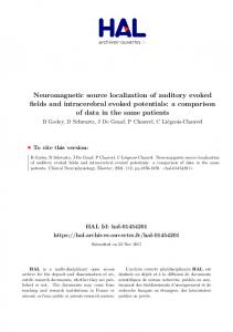
Fig. 1. Spatial map of the energy in the beamformed signal for 4 sources.

A strategy that is often applied to resolve inverse problems is the iterative generation of a sequence of forward problems that might have created the data. In the selection of the candidate forward problems, we can easily satisfy any a priori constraints. In the present case, the forward problem that is generating the data, is that there are speech source(s) in a room bounded by walls and other boundaries Thus, in applying this strategy to the present problem, we will actively search space for sources of speech. We hypothesize that there is a speech source at a particular location, performing delayand-sum beamforming with the assumed location and associated time delays, and check the validity of the hypothesis by checking the gain in the beamformed signal. We repeat this for all space points of interest, building a map of the energy in the beamformed signal for these points. An example map is shown in Fig.1, where the brightness of a pixel is proportional to the signal power when the beamformer is focused on the point. For purposes of illustration, the picture is two-dimensional and represents a simple situation when all sources are located on a plane 5 ' ~f c where 5 is normal to the plane of the array. It is clear that there are four local energetic regions, with each local peak in the energy map corresponding to the location of the source. The vertically-stretched pattern of the map is due to the distribution of microphones in our array. Using the map, the source position can be obtained easily, e.g., via a peak climbing algorithm. Of course generating a ¿ne map such as the one shown in the ¿gure will take a very long time. The accuracy of the localization is only limited by the sampling rate at the arrays and the noise in the recorded signal, and can be very precise. As presented above, the algorithm is quite unsuitable for real

1.4

time application. The goal of this paper is to show how this search can be speeded up by using a coarse-to-¿ne paradigm in both the spatial and frequency domains to achieve a practical algorithm. This strategy works only because speech has characteristic wavelengths that are comparable to the dimension of the space that is being searched. The algorithm we develop is not limited by the number of sources (though it does require them to be separated and have similar power), or the background noise structure, and has a predictable cost. It is particularly suitable for implementation in environments where there is prior knowledge of the spatial domain (e.g., the set of source locations is bounded by room walls, or the source is one of several objects detected in a room, etc.). Such knowledge could be obtained by other means such as computer vision. 2. A PRIORI INFORMATION We summarize here the a priori problem information known about the problem, and present some preliminary results that can be used to determine the coarsening strategy. Spatial extent: The source occupies a region whose spatial extent is limited. It is usually a workspace, a conference room or rarely an auditorium. In addition, sources are typically separated by distances of at least 1m, and will de¿nitely be at least 30 cm apart. Nature of the speech signal: While human hearing extends from 20Hz to 20KHz, the sound produced by the human vocal tract has signi¿cantly less range, extending from 100 Hz to 6kHz. The spectral structure of the most energetic part of speech, the voiced phonemes (which include vowels and some consonants), consists mainly of a combination of integer multipliers of a fundamental frequency sf that lies between 80-200Hz for males and 150-350Hz for females. The voiced sounds constitute the low-frequency part of the speech spectrum. The other signi¿cant contribution are stop consonants and fricative consonants with their energy around 3-5 kHz. Overall, for a speech signal we can expect components in the range 100 Hz to 6 kHz [4]. Relationship between frequency and wavelength: The equation s b ' S indicates the relationship between frequency and wavelength. The wavelengths of audible sound are comparable to the dimensions of the space we live in and to our anatomical features. Humans use the spectral cues resulting from complex scattering of sound waves on the objects of size comparable to the wavelength to determine the size of the environment and perform source localization [5]. Our goal is to exploit the relationship between speech frequency content and interesting spatial dimensions to develop fast search algorithms for locating sound sources. The table below presents some aspects of this relationship. s b Feature Remarks 20 Hz 17m Auditoriums lower hearing limit 100 Hz 3.4 m Conference rooms speech beginning 200 Hz 1.7 m Rooms, people ht. speech peak 6 kHz 5.5 cm Pinna Dimensions speech end 20 kHz 1.7 cm Concha size upper hearing limit Delay and Sum Beamforming: Given  receivers and the time delay of arrival of a signal between them,  c one can compute the beamformed signal, r c as r E|'

r E|nr2 E| 3 2 n  nr E| 3    

(1)

1.2

1

0.8

0.6

0.4

0.2

0 0

500

1000

1500

2000

2500

3000

3500

4000

4500

5000

Fig. 2. Peak width (m) as a function of frequency (Hz).

For exact time delays, compared to the signal received at any one receiver, in the beamformed signal the contributions from the source will add coherently, while signals from other locations add incoI herently. This yields a relative gain of at least  for the beamformed source. Equation (1) is expressed in the time domain. Beamforming can also be done in the frequency domain. We recall that if function r E| has Fourier transform 7 Es  cthen time shifting of r by |f modi¿es its Fourier transform as rE| 3 |f  C 7Es e2Zs |3  Equation (1) becomes 7 Es '

7 n72 e2Zs 45 n  n7 e2Zs 4Q  

(2)

Time Delay Imprecision: Given four or more receivers every point in physical space E%c +c 5 can be mapped to a point in delay space E 2 c  c e c    c    Imprecision in knowledge of the source location results in an imprecision in the computation of the delays, and the signals contributing to the beamformed signal will be only partially in phase. If the error in phase is small, then the coherence in the signals being added won’t be completely destroyed, though incoherent components will also get an addition in their energy. Elementary arguments show that for shifts at the array that are within b/5 of the correct shifts we get a greater than twofold increase in the coherent part as compared to the incoherent part. It can also be shown that for compact arrays and relatively far sources, a shift in the source position by a distance Bo results in a shift in the time delay B such that SB Bo. Thus, it is conservative to estimate that an error in the source position of b/5 will still result in a coherent gain in the beamformed signal. This is con¿rmed by tests with actual speech signals to our array. We refer to this result as the imprecision heuristic. Another way to look at this result is to plot the spatial width of the beamformed signal peak as a function of the source frequency. From simulations performed by mixing actual room recordings of speech we see that there is an inverse relationship between the peak width in the energy map and the wavelength of the sound. The peak in the energy map has a FWHM of approximately 2b*D for our array con¿guration, consistent with the above heuristic. For the frequency of 150-160 Hz (~sf  we get 2b*D E fH6. 3. ALGORITHM Let there be  microphones and let us consider beamforming a frame of  points sampled at a frequency higher than the Nyquist rate for the highest frequency in the signal. We divide space into voxels of a dimension corresponding to the coarsest size that is

consistent with a gain in energy at the lowest frequency. We then perform delay and sum beamforming at the centers of these voxels, and compare the power in the beamformed signal to that in the original signal. If there is an improvement in the received power we tag the voxel for further consideration. All tagged voxels are further subdivided in the next pass of the algorithm. There are two issues that must be ¿xed with this approach. First, at the coarse level we must restrict the beamforming to frequencies that are likely to see an improvement in their power. In addition, performing beamforming using either (1) or (2) on the full signals for even the relatively few coarse voxels will be uneconomical. A ¿rst possibility to ¿x this problem is decimation of the signal in the time domain. However, one quickly realizes that this leads to signi¿cant aliasing. An approach which achieves both goals is lowpass beamforming in the frequency domain which can be done quickly [6]. In this approach we compute the FFTs of each of the received signals at the  channels. We decimate the signal in the frequency domain (performing a lowpass operation) with a cutoff frequency determined by the voxel size at the current voxel size and compute the beamformed signal at the center of the voxels according to (2). Let there be & sources, leading to & tagged voxels. These are further divided, using the octree data structure described below, and the beamformed signal computed corresponding to delays at their centers, but now using versions of the signal that have the cutoff frequency doubled. Octrees: To perform a hierarchical division of space we use octrees. An octree is a data structure for hierarchical representation and processing of spatial data in 3D. A typical octree is organized as follows. The root of an octree is associated with a 3D region bounded by a parallelepiped (often a cube). This parent region is subdivided into eight similar equally sized octants, each carrying more speci¿c information about its portion of space. Each child octant is, in turn, recursively partitioned into eight children. The process of subdivision can continue in¿nitely, but in practice the process has to stop at a certain depth (e.g., when further subdivisions will not signi¿cantly help the search.) The hierarchical nature of octrees allows one to ef¿ciently represent and search data distributed in 3D space. The ef¿ciency arises from the fact that the size of an octree representing a 3D object volume is Er, where r is the surface of the object. Volumetric algorithms that execute on octrees rather than on voxel arrays have running times proportional to the number of blocks in the octree. This leads to the dimension reduction effect, i.e. an octree algorithm applied to a 3D problem is analogous to an array-based algorithm in 2D [7]. Implementation: Given a room with multiple sound sources, the task is to locate them using active beam forming. The algorithm proceeds by ¿rst dividing the room into voxels. The voxel size is chosen suf¿ciently small so that it is unlikely that two sound sources share the same voxel and that local maximas of the energy can be computed. The latter condition is ensured by the 2b*D heuristic. The nodes that correspond to the local maximas in the constructed energy map are selected for processing. Every node is recursively searched by partitioning it into eight children, and the child with the maximum energy level is selected for subdvision at the next level. The recursion terminates when the octree branch reaches a certain depth, corresponding to a ¿xed minimal voxel size. The procedure is repeated for about 10 levels which yields a voxel of size of about 1 cm in our implementation. The center of

the maximal energy voxel ` at the deepest level is output as the source position. A practical problem is that the actual peak may lie at the boundary of a voxel resulting in possible mislocalization of the energy maximum during the coarsest stage of algorithm. To avoid this, we perform a simple check at the last step. If at the end of the search within a voxel the peak is localized at the boundary of the original coarse voxel T , a search is also performed in the neighboring coarse voxel T  . In practice this rarely happens. Two dimensional alternative: The algorithm as described above is developed for 3D sound source localization. Often a more robust solution to performing full 3D localization is to perform angular localization with two separated arrays [8], [9]. We explore a variant of our algorithm for this situation. The search algorithm is executed in a 2D space using a quadtree-based peak search instead of an octree. This determines the bearing angles  (azimuth) and w (elevation) of the sound source relative to the arrays. The bearing estimation is done independently for the two arrays, and these are intersected to produce a 3D position. For the quadtree in the Ec w-space the quadrants are no longer rectangular in the world coordinate frame. The cutoff frequency and the initial grid size have to be selected by re-mapping the Ec w-grid to an E%c +grid using maximum possible source depth (determined by known room dimensions). 4. PERFORMANCE OF THE ALGORITHM Noisy environments: We expected the algorithm to be more robust with respect to noisy data in comparison with delay based localizers. Our intuitive rationale is that for these algorithms, one very incorrect delay estimation can throw the computed position estimation far away from the real sound source, and time delay estimation is notoriously dif¿cult in reverberant environments. While robust algorithms exist for this problem, they are relatively expensive to implement. In contrast, in our active beamforming algorithm the information processing is global, and correct delays are obtained as a result of the forward problem.

Fig. 3. Localization error (m) vs. SNR (dB) for one source. We performed several experiments with multiple sources. We recorded one of us speaking in a room with one of our array microphones, at a sampling frequency of 22.05 kHz. Thus in this data the reverberant structure of sound is the true one, and the original data is noisy. A multichannel multisource dataset is created from

by shifting the recorded signal with delays corresponding to virtual sound sources at known locations Ef& c t& c ~& To accommodate non-integer interchannel delays we interpolate the data. The signal in each channel was then contaminated randomly and independently by adding noise of different magnitudes, and then used to characterize the algorithm performance for different SNRs. The distance between the known source location and the computed location is taken to be the localization error. In Fig. 3 we present average results from 20 trials with the proposed doubly hierarchical algorithm (DHBF) for localizing one source. Also shown are results from a relatively robust delay-based algorithm (TDOA) [9]. It is clear that the new algorithm is much more robust. The algorithm gives low errors for even negative SNRs, showing that it is very robust. An objective comparison with other robust algorithms remains to be performed. Fig. 5. Algorithm time (ms) for a version of the algorithm that uses decimation in frequency (DHBF) and one that does not (SHBF) vs number of sources. Results are for 1 frame of 1024 points (50 ms of data).

Fig. 4. Localization error (m) vs. noise amplitude. Effect of adding microphones to an array, and of using two sub-arrays. Effect of number of microphones and subarrays: As mentioned previously, the robustness of the algorithm is improved by using two sub-arrays. It is also interesting to see how the algorithm performance depends on the number of channels in one sub-array. We tested our algorithm with 4 and 7 microphones in one array, and with two sub-arrays. The results are shown in Fig 4. The localization error drops signi¿cantly when data from the second microphone array is used, and only slightly when more microphones are added to one sub-array. Speed: Our algorithm can be implemented in real time. On a dual Pentium-III 933 MHz machine the algorithm works with practically no processing delay for one source, increasing to a 10% processing delay for four sources. In Fig. 5 we also show the advantage of performing decimation in the frequency domain. Without the decimation, the algorithm is not practical for real-time applications. Some further tuning can be performed on our implementation (in the way shifts are performed, and will be done later). Vision-constrained source localization Since one application area is source localization in multimodal user interface systems, a priori information from video will be available. Knowing the location of the object in the image plane of the camera we can restrict the search to areas that are likely to be sources. In our implementation of this concept, an active camera is used to scan the room. A background model is constructed from several images taken at different camera orientations and mosaicing them. The

room is constantly monitored for foreground objects, and a simple background subtraction method based on pixel intensities is used to classify every pixel as foreground/background. Since the camera image is 2D, the contour of the foreground object de¿nes a “visual cone” in which the object lies, with the cone origin at the camera center. The cone is bounded by the room walls. The union of the visual cones, L , of all objects is either used directly in a full 3D search, by ignoring voxels in the initial coarse octree which do not intersect L or, for the 2D search in Ec w space, the cone is reprojected back onto the Ec w search using known geometric relationships. In our implementation, we use two cameras, with one camera collecting the videoconferencing image from the active source, and the other camera constantly scanning the room, dynamically providing constraining data. Results from this implementation will be presented at the conference. 5. REFERENCES [1] M. Brandstein. Time-delay estimation of reverberated speech exploiting harmonic structure, J.Acou. Soc.Am., v105, 1999. [2] D. Colton & R. Kress, Inverse Acoustic and Electromagnetic Scattering Theory, Springer, 1992. [3] M. Brandstein, Explicit Speech Modeling for Distant-Talker Speech Acquisition, preprint. [4] H. Silverman. Some analysis of microphone arrays for speech data acquisition, IEEE Trans. Acoust. Speech and Signal Proc., v. ASSP-35, 1987. [5] D. Brungart & W. Rabinowitz. Auditory localization of nearby sources. Head-related transfer functions, J. Acoust. Soc. Am., v. 106, 1999. [6] P.P. Vaidyanathan. Multirate Systems and Filter Banks, Prentice Hall. 1992. [7] H. Samet. Applications of Spatial Data Structures, AddisonWesley, 1990. [8] M. Brandstein, H. Silverman. A practical methodolgy for speech source localization with microphone arrays, Computer, Speech and Language, vol. 11, 1997. [9] D. Zotkin, R. Duraiswami, L.S. Davis & I. Haritaoglu. An audio-video front-end for multimedia applications, Proc. IEEE SMC 2000, Nashville, TN, 2000.