Android Emulator with the processing capabilities set to the capabilities of a typical Android Wear device (single- core, 512MB RAM). B. Evaluation Metrics.
AdaM: an Adaptive Monitoring Framework for Sampling and Filtering on IoT Devices Demetris Trihinas, George Pallis, Marios D. Dikaiakos Department of Computer Science University of Cyprus Email: { trihinas, gpallis, mdd }@cs.ucy.ac.cy Abstract—Real-time data processing while the velocity and volume of data generated keep increasing, as well as, energy-efficiency are great challenges of big data streaming which have transitioned to the Internet of Things (IoT) realm. In this paper, we introduce AdaM, a lightweight adaptive monitoring framework for smart battery-powered IoT devices with limited processing capabilities. AdaM, inexpensively and in place dynamically adapts the monitoring intensity and the amount of data disseminated through the network based on the current evolution and variability of the metric stream. Results on real-world testbeds, show that AdaM achieves a balance between efficiency and accuracy. Specifically, AdaM is capable of reducing data volume by 74%, energy consumption by at least 71%, while preserving a greater than 89% accuracy. Keywords—Monitoring, Sampling, Filtering, Internet of Things
I.
Introduction
One of the most pressing and fascinating challenges of our time is understanding the complexity of the global interconnected world we inhabit. Recent advances in microelectronics, telecommunications and data mining have led to a growing adoption of smart devices (e.g., wearables, home monitors), which impact how we live and work [23]. These devices capture and exchange continuous data streams with other network-enabled devices, forming, what is known as, the Internet of Things (IoT). IoT devices differ from sensors as they feature processing capabilities and incorporate “smart” algorithms to produce analytic insights from raw monitoring data. Such devices can generate an unprecedented wealth of data. According to Gartner [9], 4.9 billion IoT devices will be in use by the end of 2015, up 30% from 2014, and will reach 25 billion by 2020. These billions of “things” already impact the digital universe as monitoring data generated from IoT devices accounted for 2% of the digital data in 2012 with a projection that by 2020 it will rise above 10% [19]. The “Big Data” collected from IoT devices, perceived as an essential by-product of the ICT systems that we interact with, holds the potential to scrutinize, model, and predict, individual and collective behavior in real-time. However, collecting and analysing large volumes of raw monitoring data is both resource and time consuming and may involve expensive operations such as parsing “endless” log files or performing complex queries [14] [25]. In addition, if IoT devices are battery-powered then intense
processing results in increased energy consumption and thus, less battery life [27]. Therefore, it is no wonder why taming data volume and velocity, as well as, energy efficiency, are considered as great challenges to overcome in IoT [2] [11] [17]. The remedy to reduce the volume of generated data, as well as, network traffic between IoT devices and data management endpoints, is to apply adaptive sampling and filtering techniques. Adaptive sampling is the process of dynamically adjusting the sampling rate to the current metric evolution, such that when stable phases in a metric stream are detected, the sampling rate is reduced to ease processing and energy consumption. In turn, when values of a metric stream fluctuate in time, the sampling rate is increased to notify immediately of event violations. On the other hand, adaptive filtering is the process of dynamically adapting the filter range to follow the metric evolution without requiring beforehand for users to guess what filter range should be applied. Despite advances in the field, current adaptive sampling and filtering techniques are not tailored for the challenges of IoT, since they either: (i) require excessive resources or the entire dataset to provide estimations [6] [18]; (ii) require users to provide violation likelihood thresholds [14] or filter ranges [5], which are the process of excessive profiling; (iii) assume, the metric distribution does not change in time [5] [24]; (iv) are serverside approaches and cannot be used on IoT devices [16]; or (v) are slow to acknowledge significant abrupt transient fluctuations in the metric stream distribution [7] [10]. To address the aforementioned challenges we introduce the ADAptive Monitoring (AdaM) framework. AdaM is a lightweight framework with no external dependencies developed for smart battery-powered IoT devices. AdaM, inexpensively and in place, dynamically adapts the monitoring intensity and the amount of data disseminated through the network based on the current evolution of the metric steam. By accomplishing this, energy consumption and data volume are reduced, allowing the IoT device to preserve battery and ease processing at the base station or a central endpoint, while still preserving data accuracy. To achieve this, AdaM incorporates two algorithms, one for adaptive sampling and one for adaptive filtering. Both algorithms provide one-step ahead estimations, adjusting the sampling rate and the filter range based on the confidence of each algorithm to correctly estimate what will happen next in the metric stream. Specific consideration
is taken such that our algorithms immediately identify abrupt transient changes in the metric evolution. Most importantly, AdaM runs on the source device without any additional communication to a central management endpoint and excessive profiling to determine framework parameters. In this paper, we present a thorough evaluation of AdaM by comparing it to other IoT adaptive techniques, with testbeds that utilize publicly available real-world datasets. Results, show that AdaM is capable of reducing data volume by 74%, energy consumption by at least 71%, while preserving a greater than 89% accuracy. The rest of the paper is structured as follows: Section 2 presents a study of the related work. Section 3 presents the problem statement. Section 4 introduces the AdaM framework, while Sections 5 and 6 describe our algorithms. Section 7 presents an evaluation of AdaM and Section 8 concludes this paper and outlines the future work. II.
Related Work
Edge-mining [17] is a term coined to reflect data processing on smart battery-powered devices that sit at the edges of an IoT network [10]. Adapting the monitoring intensity and the amount of information disseminated through the network, is a form of edge-mining. Current monitoring tools [8] [15] do not feature self-adaptive capabilities and therefore, are not suitable for IoT devices. In what follows, are a number of edge-mining techniques for adaptive sampling and filtering. A. Adaptive Sampling Meng et al. [14] propose a server-side solution for cloud networks where the monitoring intensity is increased when metric values approach a user-defined threshold, and is decreased when a violation is unlikely to occur. As a threshold-based technique, it fails to detect variances in the metric distribution when values are far from the threshold. Thus, it is limited only to anomaly detection. Rastogi et al. [18] propose a discrete Fourier transform (k-DFT) which perturbs coefficients of a finite timeseries, reconstructing afterwards the original timeseries from the inverse DFT. Since the entire timeseries is required, this approach is not applicable to real-time applications with continuous metric streams. Fan et al. [7] propose FAST, an adaptive framework which uses a PID controller1 to select a subset of values from a given window of samples originating from a metric stream. FAST’s adaptive sampling technique is aggressive producing large sampling periods as the purpose of its development is applying a costly user-differential policy on each interval. Thus, it requires a Kalman filter [13] which generates estimates for non-sampled intervals to reduce the estimation error. However, as the Kalman filter is used to filter signal noise, this approach does not work well for abrupt transient signals where large portions of the signal are lost due to smoothing. In addition, even for slightly less volatile signals extensive profiling of its parameters is still required to increase accuracy. In contrast to the aforementioned techniques, Gaura et al. [10] propose a number of edge mining algorithms specifically tailored to 1 https://en.wikipedia.org/wiki/PID
controller
IoT networks. With respect to adaptive sampling, Gaura et al. propose L-SIP, a linear adaptive algorithm, which encodes the state of an IoT device as a point in time with attributes the sample value and its rate of change. This is performed by using either an exponential weighted moving average (EWMA)2 or a Kalman filter, with the sampling rate increasing if the difference between the observed and prediction value, are larger than a user-defined estimation error. L-SIP is an interesting lightweight algorithm suitable for adaptive sampling on IoT devices, but exhibits two downsides: (i) it is slow to react to highly transient and abrupt fluctuations in the metric stream; and (ii) it is left to the user to determine, via profiling, which state encoding method suits best his needs. B. Adaptive Filtering From experiments on distributed systems in regards to monitoring metric variability, Clayman et al. [5] conclude that fixed filter ranges are not effective for all metrics. They suggest a monitoring system which provides the user with the ability to manually enable different filters per monitored metric. Similarly, but autonomously, Trihinas et al. [24] introduce a monitoring system capable of adjusting the filter range depending on the percentage of values previously filtered. While interesting, this approach assumes that no distribution shifts will occur in the metric evolution at runtime. Olston et al. [16] propose a server-side approach for filtering continuous data streams. This approach involves users specifying a precision requirement with data sources sending updates to a central server node when new values differ significantly from the previously reported values. If this precision requirement cannot be met, the central server will adjust the filter range at each data source. However, this adaptive filter adjustment is only feasible if data generated at different sources follow a certain similar pattern on all nodes and it assumes a one-level network often not found in IoT networks. Finally, Deligiannakis et al. [6] suggest a traffic reduction strategy for sensor networks. Their strategy considers buffering large amounts of metric values at each sensor node and, rather than transmitting the total of the buffer contents, it transmits a base signal of fewer values which is then used to reconstruct the original signal. The downside of this approach is that it requires for the whole signal to be made available and stored on the device so as to provide an estimation. In summary, there is no solution capable of estimating and adapting the monitoring intensity of an IoT device to follow in time the actual metric evolution, especially, when highly abrupt metric fluctuations are observed. III.
Problem Statement
Before diving into the specifics of the AdaM framework, it is important to understand the background that lays the groundwork for each algorithm and their respected problem definition. To ease readability, Table 1 presents the notation used throughout the paper. First, we define a metric stream M = {si }ni=0 , as a large sequence of collected samples si , where i = 0, 1, ..., n and 2 https://en.wikipedia.org/wiki/Exponential
smoothing
Notation si (t, v) M = {si }n i=0 Ti
Ri
dist
ρ(M ) q(M ) γ
Description The ith sample of a metric stream with timestamp ti and value vi Metric stream of collected samples with i = 0, 1, ..., n and n → ∞ Sampling period used to collect sample si such that Ti = ti − ti−1 and Ti is restricted to a range of values, e.g. Ti ∈ [Tmin , Tmax ] Filter range used to decide if sample si , assuming the filter window W = [vi−1 − Ri , vi−1 + Ri ], should be filtered (vi ∈ W ) or not (vi 6∈ W ) Difference between original metric stream M and reconstructed stream M 0 via an adaptive for a P technique range of sample values e.g. dist = |vi − vi0 |, i ≥ 0 Function containing information to characterise evolution of metric stream M (e.g. a moving average) Function characterising variability of metric stream M (e.g. the coefficient of variation, CV) User-defined parameter denoting the acceptable imprecision of a reconstructed metric stream via an adaptive technique (γ ∈ [0, 1])
TABLE I: Table of Notations n → ∞. Each sample si is a tuple (ti , vi ) described by a timestamp ti and a value vi . A. Adaptive Sampling Problem Definition For a metric stream M , periodic sampling is the process of triggering the collection mechanisms of a monitored source every T time units. T is a fixed interval, such that the ith sample is collected at time ti = i · T . This process is widely adopted by many monitoring tools due to its simplicity. In this work, we argue that using a fixed predefined T on battery-powered devices features a number of constraints. Specifically, it is both resource and energy consuming to collect periodically samples, especially when consecutive metric values (e.g. vi−2 , vi−1 , vi , ...) do not vary. For example, if a small T is utilized, a high volume of data is generated and must be distributed through the network to be processed or stored for further use. If, instead, a large period is used, then sudden events or significant insights may remain undetected. In general, because sampling depends on the data and its evolution in time, we argue that a fixed sampling period is not effective, as metrics and insights are only useful if collected in meaningful time intervals. To accommodate the above challenges, adaptive sampling is used. Adaptive sampling is the process of dynamically adjusting the sampling period Ti , based on some function, denoted as ρ(M ), containing information of the metric stream evolution (e.g. a moving average). Assume si to be the latest sample of M , and that Ti accepts discrete integer values in the range [Tmin , Tmax ] ⊆ Z+ without loss of generality. Now, suppose M is periodically sampled every Tmin time units, opposed to M 0 which is a reconstructed version of the original metric stream via adaptive sampling, as depicted in Figure 1. Let dist denote the difference of M 0 from M based on some distance metric. When the sample values of the metric stream are relatively stable, then the sampling period should be increased and when the values fluctuate, the sampling period should be decreased or restored to a minimum value. Hence, the goal of adaptive sampling is to provide a sampling function f (·), capable of finding the maximum T ∈ [Tmin , Tmax ] to collect si+1 , based on an estimation
Fig. 1: Adaptive Sampling Example of the metric stream evolution ρ(M ), such that M 0 differs from M less than an imprecision value γ (dist < γ) for the range t ∈ [ti , ti + T ]. Thus, the problem is summarized with the following equation: T ∗ = arg max {f (s, T, ρ(M ), dist, γ) | dist < γ, (1)
T
T ∈ [Tmin , Tmax ]} Intuitively, as γ → 0 the metric stream M 0 → M . However, the sampling period T → Tmin , defeating the purpose of adaptive sampling. To reduce data volume and preserve energy, an adaptive technique is likely to select, at any given time, a sampling period where T > Tmin , which is only applicable if a degree of imprecision is tolerable. Therefore, it is desirable to select a sampling function which achieves a balance between efficiency and accuracy. B. Adaptive Filtering Problem Definition For a metric stream M , filtering is defined as the process of “cleansing” the metric stream of collected samples such that data volume, as well as, the communication and storage overhead are reduced in favor of exact precision. Depending on the type of filter in use, the number of samples filtered may vary. For example, suppose a fixed filter range approach is followed. The sample si with value vi is filtered, if vi ∈ [vi−1 − R, vi−1 + R], where R is a fixed filter range. Although this approach is simple and followed by monitoring tools [5] [24], it features a number of disadvantages. Specifically, using a fixed filter range, assumes that the user has previous knowledge of the metric evolution and that it will not change in the future. Otherwise, there is no guarantee that any values will be filtered at all [5]. For instance, let us consider the metric stream M , presented in Figure 2, where the filter range R is enabled once and set to a small value (e.g. R = 1%). From Figure 2, we observe that although a stable phase exists in the load, with a static filter used, no samples are filtered. That is because the filter range cannot adapt to the current data variability, extending its range to encapsulate near-by values for a small imprecision sacrifice. To overcome the above issues, an adaptive filter technique is used. Adaptive filtering is the process of dynamically adjusting the filter range R based on the current variability of the metric stream (e.g. the coefficient of variation), denoted as q(M ). Adaptive filtering must target filtering values without requiring for users to “guess” what filter range should be used, as depicted in Figure 2. Thus, suppose M 0 is a reconstructed version of M with an adaptive filter range R ∈ (0, Rmax ]. Let dist denote the difference of M 0 from M based on some distance metric. After collecting si , the goal of adaptive filtering, is to
Fig. 3: AdaM Framework embedded in IoT Device Fig. 2: Adaptive Filtering Example provide a filtering function f (·) capable of finding the maximum R such that M 0 differs from M less than a user-defined imprecision value γ (dist < γ) based on the variability of the metric stream q(M ). Hence, the problem is summarized with the following equation: R∗ = arg max {f (s, R, q(M ), dist, γ) | dist < γ, (2)
R
R ∈ (0, Rmax ]} Intuitively, as γ → 0 the timeseries M 0 → M . However, the range filter R → 0, defeating even the purpose of filtering with a fixed range R. To reduce network traffic an adaptive filtering technique is likely to select, at any given time, a filter range where R > 0, which is only applicable if a degree of imprecision is tolerable. Therefore, just as with adaptive sampling, it is desirable to select a filter function which guarantees a balance between efficiency and accuracy. IV.
The AdaM Framework
To address the aforementioned problems, we have implemented in java the ADAptive Monitoring (AdaM) framework to provide adaptive sampling and filtering for IoT devices. AdaM is a lightweight framework with no external dependencies embeddable in the source code of an IoT device to self-adapt the monitoring intensity based on the current metric evolution and variability. AdaM targets reducing energy consumption, allowing the IoT device to preserve battery while achieving a balance between efficiency and data accuracy. Figure 3 depicts an exemplary IoT device with AdaM embedded in its software core. AdaM coordinates data gathering and dissemination by interacting with the Sensing, Processing and Communication Units of an IoT device. When the Sensing Unit collects a new measurement, the sample and its timestamp are passed to the adaptive sampler which returns the new estimated sampling period (Ti+1 ) and a confidence interval for the current estimation. The Sensing Unit may then use Ti+1 to collect the next sample and return to an idle state. If adaptive filtering is enabled, then the sample is forwarded to the adaptive filter to decide if the measurement should be discarded or not. In turn, the filter range Ri+1 is adjusted and an indicator of the current variability of the metric stream is provided as well. If the measurement is not filtered, AdaM will forward it to the Processing Unit for further processing or to the Communication Unit for dissemination if no further processing is required. In the following sections, we present, in detail, our adaptive sampling and filtering algorithms.
V.
Adaptive Sampling Algorithm
The following were taken into consideration while developing our adaptive sampling algorithm. First, the estimation process must be lightweight. Applying an adjustive sampling algorithm is only meaningful if the process can be done inexpensively and online. Most importantly, this process must be performed in place, right on the source device. This eliminates the need of distributing values through the network to management endpoints for it to be applicable. Moreover, it must be capable of reacting even to high abrupt fluctuations in the metric stream which may even occur after long periods of stability. Thus, users and critical decision-making processes are notified immediately of these events. In addition, extensive profiling from the user-side to identify optimal parameter configuration must not be required. We base our approach, such that the estimated sampling period Ti+1 , is dependent to the current sampling period Ti , increasing if variability of the load decreases, and, in turn, decreasing if variability increases. How large of an adjustment is required, is dependent on a confidence metric ci , denoting the confidence to estimate, correctly, the current evolution of the metric stream. Hence, in contrast to threshold-based techniques which adjust the sampling rate solely based on the sample value, our approach considers the evolution of the metric stream, as well as, the confidence of its estimation. The reason for this lays in the failure of threshold-based techniques to detect variances in the metric stream when values are far from the threshold (e.g. v[ti ] 0 then current distance δi ← |vi − vi−1 | (eq. 1) probability Pi ← probDistro(δi , δˆi , σˆi ) (eq. 8) ˆ , σi+1 δi+1 ˆ ← PEWMA(Pi , δi ) (eq. 7) compute actual observed σi ← calcSD(δi ) confidence ci ← calcConfidence(σi , σˆi ) (eq. 10)
1:
if F < γ then the metric stream is currently not dispersed and Ri+1 can be widen, else it is shortened 2:
if Ti+1 can be adjusted (either up or down) based on the determined confidence and user-defined imprecision then do so, else rollback to default Tmin 7: 8: 9: 10: 11: 12: 13: 14: 15: 16: 17: 18:
if (ci ≥ 1 − γ) then ) Ti+1 ← Ti + λ · (1 + cic−γ i if (Ti+1 > Tmax ) then Ti+1 ← Tmax end if else Ti+1 ← Tmin end if else ˆ ← v0 , σi+1 δi+1 ˆ ← 0, Ti+1 ← Tmin //init values end if return Ti+1 , µi , σi
should be considered, whereas if the evolution is small, then an increase in the sampling period can be considered. δˆi+1 = µi
(4)
Moving averages provide one-step ahead predictions. They are easy to compute, though many types exist, and can be calculated on the fly with knowledge of only the previous value, µi−1 . Equation 5 presents an example of a cumulative Simple Moving Average (SMA) where values of a sliding window are aggregated evenly: δi + (i − 1)µi−1 , i≥1 (5) i Hence, while a SMA can be used, it weighs all values the µi =
Fi ← calcF anoF actor(σi , µi )
3: 4: 5: 6: 7: 8: 9:
i Ri+1 ← Ri + λ · ( γ−F γ ) if (Ri+1 > Rmax ) then Ri+1 ← Rmax end if if (Ri+1 < Rmin ) then Ri+1 ← Rmin end if return Ri+1
same. This is not desired, as current disrupts in the metric evolution are more significant and should be valued more in a dynamic metric stream. To address this, an Exponential Weighted Moving Average (EWMA) can be used, where a weighting factor (0 < α < 1) is introduced and is used to decrease the effect of older values exponentially, as presented in Equation 6: � δi , i=1 µi = (6) αµi−1 + (1 − α)δi , i > 1 While the EWMA is a better suit for our needs it still features one significant drawback: it is volatile to abrupt changes. Therefore, the assumption made that the EWMA only changes gradually with respect to the parameterization, is not always the case [4]. Specifically, the EWMA is slow to acknowledge sudden spikes after large stable phases and, in turn, if stable phases follow sudden spikes, then spike effects preserve in the estimation. This results in overestimating subsequent δi ’s which affects the accuracy of an adaptive sampling technique. Therefore, for our proposed algorithm we adopt a variation of the EWMA, dubbed as the Probabilistic Exponential Weighted Moving Average (PEWMA) [4]. The
PEWMA dynamically adjusts the weighting based on the probability of the given observation. This method is robust to abrupt transient changes, adjusting quickly to long-term shifts in the metric evolution and when incorporated in our algorithmic estimation process, it requires no parameterization, scaling to numerous sample points. � δi , i=1 (7) µi = α(1 − βPi )µi−1 + (1 − α(1 − βPi ))δi , i > 1 Equation 7 presents the PEWMA where instead of a fixed weight factor α we introduce a probabilistically adaptable factor a˜i = α(1 − βPi ). In this equation, Pi is the probability of δi to follow a modelled distribution of the metric stream. In turn, β is a weight placed on Pi and as β → 0 the PEWMA converges to a standard EWMA. We choose to adapt weights3 α by 1 − βPi such that samples that are less likely to have been observed (e.g. sudden spikes after stable phases which do not appear again) are accounted for in the current estimation, however, offer little influence to subsequent estimations. Thus, we adopt a Gaussian signal distribution N (µ, σ 2 ), which satisfies the aforementioned requirements and therefore Pi is the probability of δi evaluated under a Gaussian distribution, which is computed by Equation 8. Figure 4 depicts a comparison between moving averages, where we observe that the PEWMA is quick to adjust to metric evolution shifts and, in contrast to the EWMA, after spikes it does not overestimate subsequent values. 1 z2 Pi = √ exp(− i ) 2 2π δi − δˆi z= σˆi
(8)
In Equation 8, δi − δˆi is the difference between the observed distance and the PEWMA estimation, while σˆi denotes the (moving) standard deviation. It is important to note, that both δˆi+1 and σ ˆi+1 , which encapsulate the current evolution of the metric stream (ρ(M )), are efficiently updated with only knowledge of their previous values and without repeatedly scanning the entire stream (n → ∞). Thus, the estimated δˆi+1 and σ ˆi+1 , are computed as follows: a˜i ← α(1 − βPi ) s1 = µi ← a˜i · s1 + (1 − a˜i ) · δi s2 ← a˜i · s2 + (1 − a˜i ) · δi2 ˆ ← s1 δi+1 q σi+1 ˆ ← s2 − s21
(9)
Having estimated the standard deviation, when the next sample is collected, the algorithm will then compute the actual observed standard deviation (step 5). This is performed, as to calculate the current confidence, denoted as ci (step 6). The confidence (ci ≤ 1) is a ratio computed from the difference between the estimated and the 3 for
simplicity in our model evaluation we consider β = 1
observed standard deviation (Equation 10) and is used as our distance metric (dist). The semantics behind the confidence are: the more “confident” the algorithm is, the larger the outputted sampling period Ti+1 can be. Hence, as σˆi → σi the confidence ci → 1. ci = 1 −
|σˆi − σi | σi
(10)
Having computed the current confidence, we then compare it to the acceptable imprecision, denoted as γ from the problem definition. The imprecision parameter (γ ∈ [0, 1]) is used to set the sensitivity of our approach while computing a new sampling period Ti+1 (Equation 11). Intuitively, if γ → 0 then our algorithm converges to a periodic sampling approach (unless an “exact” estimation is made), whereas if γ → 1 an adjustment will take place on each interval even if a confident estimation cannot be made. Hence, if the algorithm cannot provide an estimation within a certain confidence, then our adaptive sampling algorithm will rollback to the default sampling period Tmin for the next sample si+1 . ( Ti+1 =
Ti + λ · (1 + Tmin ,
ci −γ ci ),
ci ≥ 1 − γ else
(11)
The complexity of our approach is O(1) constant time, since all calculations are computed based on the previous collected values and do not require the entire metric stream to be available. Moreover, the imprecision parameter γ is the only parameter which is user-defined in the estimation process. Nonetheless, users are free to change: (i) λ which is an optional multiplicity factor (e.g. default λ = 1) to be used if a more aggressive approach should be followed; and (ii) the weighting factor α of the PEWMA, where as shown in our evaluation, α may take a wide range of values and can be left to a default value. VI.
Adaptive Filtering Algorithm
As with adaptive sampling, adaptive filtering must be lightweight and capable of running on the source device. Adaptive filtering utilizes the Fano Factor4 Fi , to compute the current variability q(M ) of the metric stream M . The Fano factor is a normalized measure of the dispersion of a probability distribution, such that it is used as a measure to quantify whether a set of samples are clustered or dispersed compared to a statistical model. The Fano factor is calculated as the ratio of the variance σ 2 to the mean µ, as presented in Equation 12: Fi =
σi2 µi
(12)
To provide both the variance σ 2 and the mean µ of the metric stream, no additional computations are required, as both µi and σi are the output of the PEWMA estimation. Intuitively, when σ 2 decreases, the Fano factor will follow, indicating a decrease in the variability of the metric stream. From the user we request at least one parameter: the maximum imprecision he is able to tolerate, if filtering 4 https://en.wikipedia.org/wiki/Fano-factor
(c) Disk I/O Trace
(b) CPU Trace
(a) Memory Trace
(d) TCP Trace
(e) Fitbit Trace
Fig. 5: Mean Absolute Percentage Error (MAPE) Comparison of Techniques Using a Moving Average Estimator
Fig. 6: AdaM γ-Parameter Evaluation is enabled, denoted (again) as γ. If Fi is less than γ, indicating the metric stream is not dispersed, then the filter range is widen, in an attempt, to filter near-by values while still in the precision indicated by the user (Equation 13). Otherwise, if Fi is greater than γ, indicating the metric stream is currently over-dispersed, the filter range is shortened or restored to a default value in order to report abnormalities in the data. γ − Fi Ri+1 ← Ri + λ · ( ) (13) γ Additional parameters which may be tweaked, include, Rmax , the maximum filter range that can be applied to R, and λ which is a multiplier, or better, an aggressiveness indicator of our approach. As with adaptive sampling, the adaptive filtering algorithm has a O(1) constant time complexity, as Ri+1 is computed from its previous value, while µi and σi are the output of adaptive sampling. VII.
Evaluation
To evaluate the functionally and effectiveness of AdaM we compare it to three state-of-the-art adaptive techniques suitable for IoT devices: (i) an exponential weighted moving average (i-EWMA) which increases the sampling
period incrementally by one time unit (Ti+1 ← Ti + Tunit ), when the estimated error � is under a user-defined imprecision value γ, and decreases it (Ti+1 ← Ti − Tunit ), when � > γ; (ii) L-SIP [10], a linear algorithm using an exponential moving average (dEWMA) to produce estimates of the current data distribution based on the rate sample values change in time; and (iii) FAST [7], a framework which uses a PID controller to determine the sampling period accompanied by a Kalman filter to predict values at non sampling points. FAST’s Kalman filter parameters are tuned for each trace, as its formulation is highly dependent to data velocity. For all techniques, including AdaM, we set the acceptable imprecision to γ = 0.1. A. Traces and Testbeds In what follows is a list of the datasets we have selected to evaluate the under comparison techniques. Instead of using simple trivial traces (i.e. stable, linear or sinusoidal load), we have selected five publicly available real-world complex traces to truly reveal the strengths and disadvantages of each algorithm: • (Memory Trace): A memory trace of 105 samples originating from a java sorting benchmark [12]. • (CPU Trace): A CPU trace of 800 samples originating from the Carnegie Mellon RainMon project [22]. • (DiskIO Trace): A Disk I/O trace of 415 samples from the Carnegie Mellon RainMon project [22]. • (TCP Trace): An incoming TCP network traffic trace of 500 samples from the port activity monitor of the Cyber Defense SANS Technology Institute [20]. • (Fitbit Trace): A fitness trace of 287 samples from a Fitbit device as part of a Coursera data science course [1]. The experiments for the first four traces were run on a Raspberry Pi (1st gen, Model B) with 512MB of RAM and an ARM processor (single-core, 700MHz) while emulating the data load of each trace. The Raspberry Pi was
(b) CPU Trace
(a) Memory Trace
(d) TCP Trace
(c) Disk I/O Trace
(e) Fitbit Trace
Fig. 7: A Comparison of Traces Generated via AdaM Towards the Original Traces selected as a suitable testbed, as it features similar limited processing capabilities of other “smart” devices, such as home monitors, wireless sensors and activity trackers. The Fitbit Trace was fed, via SensorSimulator [21], to the Android Emulator with the processing capabilities set to the capabilities of a typical Android Wear device (singlecore, 512MB RAM). B. Evaluation Metrics We evaluate each technique towards: (i) their estimation accuracy, by calculating the mean absolute percentage error (MAPE) from the original timeseries which is the ground truth for each trace. Equation 14 depicts how the MAPE is calculated, where Ai is the actual value for the ith sample and Ei is the estimated value. We note that, for each sampling technique when a sample is not collected, Ei is considered the last reported value; (ii) CPU cycles, required to process the load imposed by each trace; (iii) outgoing network traffic, where for simplicity we assume that no aggregation technique is available and therefore each collected sample, if not filtered, is disseminated to the remote base station; and (iv) energy consumption, based on the model adopted from [27] and power measurements acquired with the help of powertop5 and wattch [3]. Equation 15 presents the adopted energy model, where Pidle denotes the power in idle state; Pcpu , the power of the processor (including CPU, L1 cache and memory); τcpu , the CPU time; Pi/o , the power for I/O; τcpuwait , the I/O time; while Pnet , the power consumed when distributing packets over the network. n
1 X Ai − E i M AP En = | | · 100% n i=1 Ai
(14)
E = Pidle · τidle + Pcpu · τcpu + Pio · τcpuwait + Pnet · τnet (15) 5 https://01.org/powertop
C. Experiments At first, we compare AdaM’s sampling algorithm to i-EWMA and L-SIP towards the MAPE metric. These three algorithms use moving averages in their estimation process and, therefore, we evaluate MAPE under different configurations for the moving average parameter α to find the best configuration. We define the minimum sampling period to be 1 time interval, which is equal to the sampling period used to collect the ground truth for each trace, while the maximum sampling period is set to 10 intervals. It must be noted that we do not present FAST in this test. This is due to FAST not using a moving average, but most importantly, its sampling is aggressive producing only a few sampling points and without filtering its MAPE is very high. Therefore, a test without filtering enabled, is meaningless. To be fair, we present its MAPE in subsequent comparisons while enabling filtering (see Fig. 8d). Figures [5a-5e] depict the MAPE metric of each trace for the under comparison techniques. First, we observe that AdaM (λ = 1) in all five traces has the smallest error. In its best configuration, AdaM’s MAPE, is under 10% except for DiskIO trace, where it is slightly above. Even, in a more aggressive configuration (λ = 2) AdaM still achieves a low error percentage and is comparable to L-SIP. AdaM’s sampling algorithm achieves a low MAPE due the ability of the PEWMA estimation to immediately detect abrupt transient changes in each trace. Moreover, we observe that AdaM’s sampling algorithm can take a wide range of values for the α parameter (e.g. α ∈ [0.3 − 0.6]) with a deviation under 5% from the best configuration. This is important as profiling to find the optimal configuration is not required if a slightly increased imprecision is acceptable. In turn, Figure 6 depicts the importance of the confidence metric as in all imprecision configurations and for all traces, AdaM’s MAPE is way below the maximum acceptable imprecision threshold (M AP E < γ), even for γ-values which indicate a high error tolerance. Furthermore, Figures
(a) CPU Cycles
(b) Energy Consumption
(c) Outgoing Network Traffic
(d) Mean Absolute Percentage Error (MAPE)
Fig. 8: Overhead Comparison of the Techniques Under Evaluation [7a-7e] depict AdaM sampling algorithm compared to the original traces, where we observe that AdaM always follows the data evolution even in highly fluctuating phases. Thus, we consider the depicted timeseries as identical. Next, as depicted in Figures [8a-8d], we compare all algorithms based on the overhead imposed to the IoT device they are deployed on. In this comparison we include FAST, as well as, AdaM (λ = 1) with filtering enabled. At first, we observe (Fig. 8a) that filtering does not impose additional overhead to AdaM as the overhead in all cases is under 2%. However, the gains from reduced network traffic (Fig. 8c) are significant as an average reduction of 69% is achieved. In turn, even with filtering enabled, accuracy is preserved (Fig. 8d) as the error is never increased more than 6%. In general, when comparing AdaM to periodic sampling, AdaM succeeds in reducing data volume by 74%, energy consumption by at least 71%, while accuracy is, in all cases, greater than 89% and with filtering enabled, greater than 83%. Moreover, as with MAPE, we observe that AdaM outperforms i-EWMA and L-SIP. Specifically, from the baseline (periodic sampling), L-SIP reduces network traffic by 36% and achieves a 44% reduction of energy consumption. AdaM is able to achieve this due to its low complexity (O(1)) and the introduction of the confidence metric which supports the estimation process to select the appropriate T . Nonetheless, its overhead is slightly larger than the FAST algorithm. FAST’s aggressiveness, which computes larger sampling periods, results to slightly lower energy consumption and network traffic. However, this
does not come for free. From Figure 8d we observe that for FAST to achieve low energy consumption and network traffic, significant accuracy is sacrificed, in contrast to AdaM which even with filtering enabled, achieves a balance between efficiency and accuracy. D. Scalability Evaluation In the next experiment, we intend to showcase the benefits of integrating AdaM with data streaming sources in regards to the velocity of which data is generated. Specifically, we take advantage of the open-source JCatascopia Monitoring System [24], where we embed AdaM in the source code of its Monitoring Agents, such that they are capable of adapting the sampling rate and the metric filter range. As data sources we create Monitoring Probes which upon initialization, they randomly select 1 of the 5 traces introduced earlier to emulate its behavior. For each trace we set the minimum sampling period to 1s, in order to generate a high volume of data. We use these traces, and not random data as we have confirmed, from our evaluation, that AdaM can reconstruct each of the available traces with high accuracy. At first, our topology is comprised of 1 data source and every 5 minutes a new data source is instantiated until we reach a capacity of 80. Metrics are disseminated to a single Monitoring Server (4VCPU, 4GB RAM) where they are processed. We study data velocity by measuring archiving time, which is the average time required by the Monitoring Server to process and store a received metric to its database. Figure 9 depicts the results of our comparison, where we observe that without any adaptive
[6]
[7]
[8] [9]
Fig. 9: Scalability Evaluation sampling technique data velocity follows an exponential growth. However, if data sources utilize AdaM’s adaptive capabilities, data velocity is reduced and a linear growth is achieved. VIII. Conclusion and Future Work In this paper, we have introduced AdaM. AdaM is an adaptive monitoring framework for smart IoT devices, which, inexpensively and in place, dynamically adapts the monitoring intensity and the amount of data disseminated through the network based on the current metric evolution. AdaM’s algorithms make this possible by providing onestep ahead estimations to adjust both the sampling rate and the filter range based on the confidence of each algorithm to correctly estimate what will happen next in the data stream. With real-world complex testbeds, we show that in contrast to other techniques, AdaM achieves a balance between efficiency and accuracy, as it is capable of reducing data volume by at least 74%, energy consumption by at least 71%, while preserving a greater than 89% accuracy. In turn, data velocity is significantly reduced, offering IoT networks greater scalability. As future work, we intend to fully integrate Adam to JCatascopia, and enhance it with further intelligent estimation techniques (i.e. metric correlation identifier). These techniques will accept additional input (i.e. data seasonality, user hints, etc.) to enrich the knowledge base used by our algorithms, in order to provide accurate Nstep estimations, not just for IoT devices but even for distributed data streaming engines as well. IX.
[3]
[4]
[5]
[11]
[12] [13] [14]
[15] [16]
[17]
[18]
[19] [20] [21] [22]
Acknowledgement
This work was partially supported by the EU Commission in terms of the PaaSport 605193 FP7 project (FP7SME-2013). References [1] [2]
[10]
Analyzing FitBit Data, https://rpubs.com/dmaurath/24643. L. Atzori, A. Iera, and G. Morabito, “The internet of things: A survey,” Computer Networks, vol. 54, no. 15, 2010. D. Brooks, V. Tiwari, and M. Martonosi, “Wattch: a framework for architectural-level power analysis and optimizations,” in Computer Architecture, 2000. Proceedings of the 27th International Symposium on, June 2000, pp. 83–94. K. M. Carter and W. W. Streilein, “Probabilistic reasoning for streaming anomaly detection,” in Statistical Signal Processing Workshop (SSP), 2012 IEEE. IEEE, 2012, pp. 377–380. S. Clayman, R. Clegg, L. Mamatas, G. Pavlou, and A. Galis, “Monitoring, aggregation and filtering for efficient management of virtual networks,” in Proceedings of the 7th Int. Conference on Network and Services Management, 2011, pp. 234–240.
[23] [24]
[25]
[26]
[27]
A. Deligiannakis, Y. Kotidis, and N. Roussopoulos, “Compressing historical information in sensor networks,” in Proceedings of the 2004 ACM SIGMOD International Conference on Management of Data, ser. SIGMOD ’04. New York, NY, USA: ACM, 2004, pp. 527–538. L. Fan and L. Xiong, “Real-time aggregate monitoring with differential privacy,” in Proceedings of the 21st ACM International Conference on Information and Knowledge Management, ser. CIKM ’12. New York, NY, USA: ACM, 2012, pp. 2169–2173. Ganglia, http://ganglia.sourceforge.net/. Gartner Says 4.9 Billion Connected ”Things” Will Be in Use in 2015, http://www.gartner.com/newsroom/id/2905717. E. Gaura, J. Brusey, M. Allen, R. Wilkins, D. Goldsmith, and R. Rednic, “Edge Mining the Internet of Things,” Sensors Journal, IEEE, vol. 13, no. 10, pp. 3816–3825, Oct 2013. J. Gubbi, R. Buyya, S. Marusic, and M. Palaniswami, “Internet of Things (IoT): A Vision, Architectural Elements, and Future Directions,” Future Gener. Comput. Syst., vol. 29, no. 7, pp. 1645–1660, Sep. 2013. Java Microbenchmark Kit, https://goo.gl/zRTQDv. R. E. Kalman, “A new approach to linear filtering and prediction problems,” ASME Journal of Basic Engineering, 1960. S. Meng and L. Liu, “Enhanced Monitoring-as-a-Service for Effective Cloud Management,” Computers, IEEE Transactions on, vol. 62, no. 9, pp. 1705–1720, Sept 2013. Nagios, http://www.nagios.org/. C. Olston, J. Jiang, and J. Widom, “Adaptive filters for continuous queries over distributed data streams,” in Proceedings of the 2003 ACM SIGMOD International Conference on Management of Data, ser. SIGMOD ’03. New York, NY, USA: ACM, 2003, pp. 563–574. C. Perera, C. Liu, and S. Jayawardena, “The Emerging Internet of Things Marketplace From an Industrial Perspective: A Survey,” Emerging Topics in Computing, IEEE Transactions on, vol. PP, no. 99, pp. 1–1, 2015. V. Rastogi and S. Nath, “Differentially private aggregation of distributed time-series with transformation and encryption,” in Proceedings of the 2010 ACM SIGMOD International Conference on Management of Data, ser. SIGMOD ’10. New York, NY, USA: ACM, 2010, pp. 735–746. Rich Data and the Increasing Value of the Internet of Things, http://goo.gl/sfk1hW. SANS Technology Institute, https://isc.sans.edu/port.html. Sensor Simulator, https://goo.gl/3pOaSQ. I. Shafer, K. Ren, V. N. Boddeti, Y. Abe, G. R. Ganger, and C. Faloutsos, “Rainmon: An integrated approach to mining bursty timeseries monitoring data,” in Proceedings of the 18th ACM SIGKDD International Conference on Knowledge Discovery and Data Mining, ser. KDD ’12. New York, NY, USA: ACM, 2012, pp. 1158–1166. The 10 most popular Internet of Things applications right now, http://iot-analytics.com/10-internet-of-things-applications/. D. Trihinas, G. Pallis, and M. Dikaiakos, “JCatascopia: Monitoring Elastically Adaptive Applications in the Cloud,” in Cluster, Cloud and Grid Computing (CCGrid), 14th IEEE/ACM International Symposium on, May 2014, pp. 226–235. O. Vallis, J. Hochenbaum, and A. Kejariwal, “A novel technique for long-term anomaly detection in the cloud,” in 6th USENIX Workshop on Hot Topics in Cloud Computing (HotCloud 14). Philadelphia, PA: USENIX Association, Jun. 2014. Y. Xiang, K. Li, and W. Zhou, “Low-rate ddos attacks detection and traceback by using new information metrics,” Information Forensics and Security, IEEE Transactions on, vol. 6, no. 2, pp. 426–437, June 2011. Y. Xiao, R. Bhaumik, Z. Yang, M. Siekkinen, P. Savolainen, and A. Yla-Jaaski, “A system-level model for runtime power estimation on mobile devices,” in IEEE/ACM Int’l Conference on Cyber, Physical and Social Computing (CPSCom), Dec 2010, pp. 27–34.