Justinian P. Rosca, Dana H. Ballard. The University of ... dividuals) are genetically bred (similarly to the GA approach), based on three genetic operations: ...
Genetic Programming with Adaptive Representations Justinian P. Rosca, Dana H. Ballard The University of Rochester Computer Science Department Rochester, New York 14627 Technical Report 489 February 1994
Abstract Machine learning aims towards the acquisition of knowledge based on either experience from the interaction with the external environment or by analyzing the internal problem-solving traces. Both approaches can be implemented in the Genetic Programming (GP) paradigm. [Hillis, 1990] proves in an ingenious way how the rst approach can work. There have not been any signi cant tests to prove that GP can take advantage of its own search traces. This paper presents an approach to automatic discovery of functions in GP based on the ideas of discovery of useful building blocks by analyzing the evolution trace, generalizing of blocks to de ne new functions and nally adapting of the problem representation onthe- y. Adaptation of the representation determines a hierarchical organization of the extended function set which enables a restructuring of the search space so that solutions can be found more easily. Complexity measures of solution trees are de ned for an adaptive representation framework and empirical results are presented.
This material is based on work supported by the National Science Foundation under Grant numbered IRI-8903582 by NIH/PHS research grant numbered 1 R24 RR06853-02 and by a Human Science Frontiers Program research grant. The government has certain rights in this material.
1 Introduction The de ning characteristic of a learning system is considered to be the capability of adaptation under the implicit goal of performance task improvement [DeJong, 1988]. The adaptation process subsumes structural changes, discovery and use of new concepts. Our focus is the Genetic Programming paradigm, as de ned in [Koza, 1992]. In GP, evolution can be viewed as structure synthesis, where the format of the structure is in terms of programs. However changing individual program instructions is most often unfruitful, so extensions to GP have tried to randomly de ne and use larger components such as new functions (automatic function de nition or ADF in [Koza, 1992]) or modules (in [Angeline and Pollack, 1994]). This paper presents an alternative approach to structure synthesis di�erent from either ADF or modules in several respects. We show that e�cient structure synthesis can be obtained by discovering useful genetic material and using it globally to adapt the problem representation. The process of discovery is based on an analysis and tracking of substructures called building blocks over generations of evolution. We describe how building blocks result from several heuristic criteria for extending the problem representation. These are used to extend the GP paradigm in what we call Adaptive Representation (AR) GP. In the next section we present an overview of the GP paradigm, and an example of applying its main steps to evolve a population of programs that solve the even-parity problem. We also summarize related work and analyze in more detail two extensions to GP, automatic de nition of functions and module acquisition. In section 4 the main theoretical concepts of the GA literature (schemata, schemata theorem, implicit parallelism) form the basis for an approach to analyze genetic material in GP. We de ne the concepts of GP blocks and building blocks and show that the interpretations given provide the foundation of a theory for adapting problem representation and making GP search more e�cient. Section 5 presents two alternative methods for analysis of candidate building blocks. The Adaptive Representation (AR) GP algorithm and details on its implementation are presented next. The ideas introduced are analyzed in section 7 using even-parity as a test case. Conclusions and future work directions are nally presented.
2 Overview of the GP Paradigm A concise description of the paradigm, its main parameters and discussions of some advanced topics are presented in [Koza, 1992], [Koza, 1994]. Here we just overview some basic concepts and notations used throughout this paper. In GP, problem solving is formulated as a search in the space of computer programs, structures of dynamically varying size and shape. Populations of computer programs (individuals) are genetically bred (similarly to the GA approach), based on three genetic operations: Reproduction, crossover and mutation (Or , Oc and Om respectively). Each operation is based on a selection of t individuals. The tness of any individual is determined by evaluating the individual program using domain dependent performance/cost functions (C ). A useful measure is normalized tness. If performance of individual i is c(i) � 0 (also called standardized tness) then a normalized 1
tness measure of individual i is Pc(ic)(i) . Normalized tness can be also de ned based on i ranking [Winston, 1992] or other ad-hoc methods. Two selection methods are currently used. A rst one, tournament selection, is described in [Angeline and Pollack, 1993a]. We randomly choose a small group of individuals and let them play a \tournament". The winner represents the individual selected. For example, the competition can consist only of tness comparison: the individual with the best tness value among the ones in the competing group is declared the winner. A second method is tness proportionate reproduction: An individual is selected with a probability proportional to its normalized tness value. Reproduction is the process of copying individuals according to their tness value. Crossover is the process in which two new programs result from an exchange of genetic material between two old programs. It consists of three steps. First, two winner individuals are selected from the population. Then a node called pivot is randomly chosen in the tree representing each winner. Finally, subtrees rooted at the two pivots are swapped. Mutation is the process in which a newly generated subtree replaces the subtree rooted at a random pivot position in a selected individual. The population tness evaluation, reproduction, and genetic recombination steps are repeated until a termination criterion is met (usually when a good enough individual is discovered or a big enough number of generations is consumed). The initial steps in applying GP to evolve a population of programs for solving a given problem are: (1) de ne the set of program primitives (initial genetic material), namely the set of terminals T and the function set F0; (2) de ne the evaluation (cost or merit) measures C and the set of tness cases E on which individual programs are tested. E can represent an evolving population too, as in the parasites metaphor (see [Hillis, 1990]); (3) de ne the control parameters (population size M , maximum number of generations G, selection method, fractions of individuals on which each genetic operator is applied, etc.); (4) de ne a termination criterion (new generations of individuals are created until this criterion is satis ed). Once these are determined an extended GP algorithm can be applied. The structure of such an algorithm is given in gure 1. Elements marked (� ) are part of our extended algorithm that copes with the automatic adaptation of the problem representation and will be explained later.
2.1 An example: learning the EVEN-n-PARITY function The problem chosen to test the ideas in this report is learning the boolean even parity function of a number n of arguments (bits), even-n-parity. This function appears to be di�cult to learn in a GP implementation especially for values of n greater than 5 [Koza, 1992]. Formally, the even-n-parity problem is to nd a functional program representing a logical composition of primitive boolean functions that computes the sum of input bits over the eld of integers modulo 2. Four primitive boolean functions of two variables make up the function set: F0 = fAND; OR; NAND; NORg 2
GP skeleton
De ne problem: T F0 C E , (� )CBB (block tness functions). Denote the population at a given generation by Pi . 1. Initial Generation: = 0 2. Randomly initialize population P0(T F0) 3. Repeat until termination criterion is met (generation ) (a) Evaluate population(Pi E C ) (b) Generate a new population Pi+1 by reproduction, crossover, mutation of individuals(Pi) i. Select genetic operation ( r c m ) ii. Select winning individuals W from current population ( Pi) iii. Generate o�spring( ,W ,Pi+1) (c) (� )Adapt representation(Pi Fi Fi+1) (d) (� )Enrich population Pi+1 (T Fi+1, epoch-replacement-fraction) (e) Next generation: = + 1 ;
;
;
i
i
;
i
;
;
O
O ;O ;O
O;
O
;
;
;
i
i
Figure 1: Skeleton of a GP algorithm The terminal set is de ned by a set of boolean variables:
T = fD ; D ; D ; :::; Dn? g 0
1
2
1
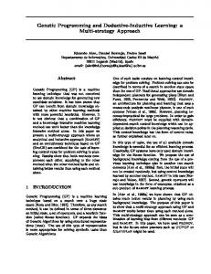
For example the tree in gure 2 represents a LISP program implementing a boolean function of 3 variables built on the basis of F0 and T = fD0; D1; D2g. Any boolean function of n variables is de ned on the set of 2n combinations of input values. Given a program implementing a boolean function, we compare its performance on all possible combinations of boolean values for the input variables against a table de ning the even-n-parity function. The table represents the set of tness cases E . Similarly to supervised learning techniques, it tells when the answer given by a program is correct. Each time the program and the even-n-parity table give the same value, the program records a hit. GP searches (in the space of all possible programs de ned by such trees) for a program that has the maximum number (2n ) of hits. The cost or standardized tness of a program i having Hits(i) hits, and a size Size(i) is: Craw (i) = (2n ? Hits(i)) � C 1 + Size(i) � C 2 (1) where C 1; C 2 are constants. The size of a program represents its structural complexity, and is de ned as the number of function points (inner nodes) and terminal points (leaf nodes) in the tree representing the program. The notion of structural complexity will be generalized later for programs that call non-primitive functions. 3
Taking C 1 = 1 and C 2 = 0 corresponds to a simple tness function based only on hits. A low value of the standardized tness function is better than a higher value. According to this measure, we look for individuals with a zero tness value. In the general case the termination criterion is satis ed if a perfect individual, i.e. one having the maximum number of hits, is found or a maximum generation number is reached. When C 2 6= 0, then for the same number of hits, individuals with a smaller size will have a lower overall tness value and will be preferred to individuals with a bigger size. In this case the tness function incorporates a size pressure component.
Figure 2: Example of solution to the EVEN-3-PARITY problem Figure 2 actually represents the solution tree obtained for a run of even-3-parity after 23 generations. It implements a boolean function computing parity on 3 input bits. The size of the search space in GP is equal to the number of program trees of depth at most D (an initial parameter of GP) that can be generated. A lower bound on this value is given by the number of complete binary trees having leaf labels from T and inner labels from F : j F j2D ?1 � j T j2D . Regardless of the symmetry or other properties of the problem domain, the number of solution trees is much smaller than this value, fact which explains why searching for solutions is a very hard problem. In addition the sparseness in solutions of the search space increases as the problem is scaled up, as is the case with the results for many problems reported in [Koza, 1994]. The question is then how can we improve the performance of GP for very sparse solution spaces? 4
3 Related Work In the next two sections we summarize two extensions to GP that point out the possibility of evolution of new functions [Koza, 1992] or emergence of modules [Angeline and Pollack, 1994] as possible ways to cope with complex problems.
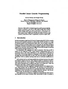
3.1 Automatic de nition of functions Automatic de nition of functions (ADF) is an extension of the GP paradigm to cope with the automatic decomposition of a solution function [Koza, 1992]. In ADF-based GP each individual has a xed number of components: functions to be automatically evolved (having a xed number of parameters) and result producing branches. Each component is a piece of lisp code built out of speci c primitive terminal and function sets, and is subject to genetic operations. Functions represent fragments of code that can be called in the program itself, playing the role of reusable subroutines. Evolution of de nitions for the functions as well as of the program body is a result of the tness pressure on population individuals. Let us take a program pattern with two automatically de ned functions (ADF0 and ADF1) and a result producing branch with one body. Then one has to distinguish between terminal sets and function sets for the body of ADF0, the body of ADF1 and the program body. In the example presented in gure 3 terminals from the initial terminal set are not included in the terminal sets for the function branches. The primitive function and terminal sets are de ned such that the components form a xed hierarchy. Genetic operations are constrained depending on the components on which they operate. For example crossover can only be performed between components of the same type. Although the hierarchy of components is xed, it boosts the power of solution discovery especially for problems with regular solutions or decomposable into smaller subproblems. A generalization of ADF, hierarchical automatic de nition of functions, answers a natural question regarding the default structure of the function sets for ADFs: lower order ADFs can be called from higher order ADFs. GP extended with ADFs (ADF-GP) is theoretically not more powerful than standard GP but it is more e�cient. Two main di�erences are: First ADF-GP develops much more complex programs. The size of the program body would \explode" if we did an inline substitution of ADF down to the basic primitives in the program body (see the de nition of the expanded structural complexity notion in section 5). Secondly ADF-GP is able to make larger jumps in the search space. For example a mutation in the lowest ADF level, ADF0, called in higher level ADFs radically changes the behavior of the body of the program. The size of trees is kept reasonably down, while the power of the resulting program is increased. Note that functions are not shared between individual programs. Functions may have no clear meaning from the point of view of the problem solved, they may not correspond to speci c subgoals related to the problem at hand. We do not a priori know what a subproblem is. Functions are not explicitly associated to problem subgoals even in the case when we know what a problem subgoal is. Ultimately, the e�ort to tune up the architecture may not be negligible. 5
ADF0
ADF1
PROGRAM-BODY
ADF1 ADF0 ADF0
ADF0 ADF0 A = {Arg0, Arg1}
A = {Arg0, Arg1, Arg2}
F = {OR, AND, NOR, NAND}
F = {OR, AND, NOR, NAND, ADF0}
T = {Arg0, Arg1}
T = {Arg0, Arg1}
ADF1
F = {OR, AND, NOR, NAND, ADF0, ADF1}
T = {D0, D1, D2}
Figure 3: An individual program with two automatically de ned functions. It consists of three branches: ADF0, ADF1 and a result producing branch with one body. Each branch has a set of arguments A (only for ADFs), a function set F and a terminal set T which are established in the problem de nition The main advantages of the approach are its generality, exibility, and performance as proved in many examples ([Koza, 1994], [Kinnear, 1994]). ADF-GP automatically discovers how to decompose a problem into subproblems how to solve the subproblems (ADFs) and how to combine the solutions to subproblems (in higher level ADFs and program body).
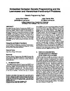
3.2 Module acquisition The module acquisition approach [Angeline and Pollack, 1993b] is applied more generally to evolutionary algorithms (an umbrella term covering GP and Evolutionary Programming). The ideas implemented within the genetic programming paradigm are illustrative and will be described shortly here. This approach is based on the creation and administration of a library of modules which extend the problem representation and on the use of two new genetic operators, compress and expand [Angeline and Pollack, 1994], that control the process of modifying population individuals. A module is a function with a unique name de ned by selecting and chopping o� branches of a subtree selected randomly from an individual. The function's parameters are determined by the places where the tree is trimmed. The module's name is used to extend the basic language. The compress operator randomly chooses a node in a program tree and extracts a module from it. Expand, implements the inverse function of compress. It simply expands a selected module name with the module itself back into the program tree where it was created. Compression freezes possibly useful genetic material, by protecting it from the destructive e�ect of other genetic operators [Angeline and Pollack, 1993b]. It also increases the expressiveness of the base language and helps in decreasing the average size of individuals 6
in the population, while maintaining the same power. As a side e�ect, if used alone, it may generate a loss of diversity in the population. The expansion operator overcomes this problem (see gure 4.) Compress
Compressed program tree
Mod
Program tree Expand F1 F6
T2
F7
F3
F2
T2
T1
F4
T3
T2
T3
F5 F1
F6
F7
Mod(arg1, arg2, arg3)
T2 F2
T2
T3
T3
F3
T2 T1
F5
F4
arg1
arg2
arg3
Figure 4: Operators de ning the modules approach It is interesting that in [Angeline and Pollack, 1994], the authors talk about the worth of a module, but they attribute to it a rather passive role. The module's worth is the number of times the module has been used since its birth, in subsequent generations. If a module is not frequently used, it means it is not viable in the competition with other individuals. The authors need a way to discard modules, as their number increases tremendously, and module usefulness seems to be an intuitive criteria. One of the problems with this approach is that the representation is extended with too many modules, most of which are unuseful. Moreover, a library of modules has to keep track of all these modules, increasing memory requirements and overhead. Problem speci c modularizations emerge, but they might have no meaning from the application's point of view. A performance comparison of ADF and module acquisition is presented in a recent paper [Kinnear, 1994]. The author analyzes the performance of the two methods and many other variations of the methods and attributes the better performance of ADF to the repeated use of calls to automatically de ned functions and to the multiple use of parameters. An attempt to explain the course of evolution in GP based on an understanding of what building blocks are appears in [Tackett, 1993]. The idea that frequent subtrees in one individual correspond to synthesized features suggests the conclusion that those subtrees comprise \building blocks". 7
4 Building Blocks We will cope with some of the problems of these earlier approaches. Most importantly we will give a clear interpretation of what good fragments of genetic material are. GP can take advantage of its own evolutionary trace in order to discover good genetic material and use it to adapt the search process.
4.1 Foundations In Genetic Algorithms (GA), the schemata theorem [Holland, 1992], [Goldberg, 1989] summarizes the e�ect of tness-proportionate reproduction, crossover and mutation. Schemata are template strings representing sets of individuals in the search space. Schemata are de ned by strings over the (usually binary) alphabet extended with a don't care symbol. The importance of schemata lies in the characterization of how GAs work, both at the representation and processing levels. The schemata theorem proves that individuals that match short de ning length (distance between the rst and the last speci c string positions) schemata with tness values above population average will be selected in an exponentially increasing number of samples in the next generations. Thus at the representation level, schemata outline the role of building blocks. A building block is a schema of short de ning length whose de ned positions tend to improve the behavior of individuals that match it and which describes fragments of a nal solution. Individuals in the population provide a partial evaluation of schemata they match. GAs work best when the internal representation encourages the emergence of useful building blocks that can subsequently be combined with each other to improve performance. At the processing level schemata outline the implicit parallelism of GAs. A population of M individuals actually samples O(M 3 ) schemata (for binary representations). Individuals in the population provide a partial evaluation of schemata they match. GAs work best when the internal representation encourages the emergence of useful building blocks that can subsequently be combined with each other to improve performance. [Davidor, 1989] outlines that choosing a representation for a GA is more of an art. The schemata theorem provides only general rules, it does not assess the suitability of a representation. Epistasis (concept derived from the Greek words \epis" - stand, and \stasis" - behind) describes gene interaction, and can be theoretically used as a measure of suitability of a representation. The design of a good representation should reconcile two con icting goals: allow easy exchange and variation of genetic material and de ne operators that preserve as much genetic material form the parent strings as possible [Deugo and Oppacher, 1990]. [Antonisse, 1989] argues for the idea that a more expressive alphabet carries more power in an informationally equivalent environment. He uses a di�erent interpretation of schema notation, in which don't care symbols quantify over subsets of symbols that can occupy a given string position. Informational equivalence means that the same number of distinct strings can be speci ed using each of the di�erent alphabets. The power of an alphabet is given by the number of schemata sampled by each individual in the population. 8
GP provides a very natural and well understood representation for a program in the form of a parse tree. This is one of the reasons for which LISP appears to be a suitable high level language for implementing the GP paradigm. The epistasis idea can not be easily applied to GP approaches, where the interaction of parts of a program is very hard to decipher. Moreover, no precise de nition of a GP schema exists, and no alternative schemata theorem has been proven for GP. One more di�culty is outlined in [Angeline, 1994]. GP individuals represent code, as opposed to the GA representation. There exists a complicated many-to-many mapping between genotypic and phenotypic features. In the next section we de ne the concepts of blocks and building blocks and show that the interpretations given provide the basis of a theory for adapting problem representation and making the GP search more e�cient.
4.2 Building blocks in GP An individual in GP is a piece of \code" in a base language (lisp in our experiments). Although the interactions between the di�erent fragments of code may be very entangled, we argue in favor of the natural formation of genotypic features, or GP building blocks. We de ne blocks as entire subtrees of a given maximum height from population individuals. This represents the bottom-up approach in gure 5. (In contrast, the module approach [Angeline and Pollack, 1994] starts with subtrees of any depth and chops o� all branches at a given depth.) We will show that the bottom-up approach enables the de nition of blocks whose usefulness can be evaluated. A key idea is that although it may be important to keep track of blocks of arbitrary size, only monitoring the merit of small blocks (with height less that gmax) is feasible. Furthermore useful blocks tend to be small and the process can be applied recursively to discover more and more complex blocks. A block can be generalized by substituting each occurrence of a terminal of the block by a variable (descriptive generalization in [Michalski, 1983]). This process transforms a block into a parameterized function whose parameters are given by the block variables. Figure 5 presents an example of a function Fb generated in this approach. Steps 3a and 3b from gure 6 implement this idea (see section 6). By analogy with Goldberg's de nition, a GP building block corresponds to a parameterized piece of code that, once used as a problem primitive, has noticeable good e�ect on the behavior of the individuals. Thus, a good building block has the potential to successfully extend the set of function primitives of the problem. For a comparison with GA, note that if we place in the initial population individuals that match a-priori known useful schemata, the convergence of the GA improves drastically. We explain this by the reduction in dimensionality of the search space caused by the \biased" initial population (GA). In GP such an improvement could be explained by the more powerful set of primitives. The goals we aim at next are the discovery of new functions based on an analysis of blocks that leads to candidate building blocks and the dynamic extension of the function set with these new functions created on-the- y from promising blocks. We call such a representation an adaptive representation, as it is automatically changed while the GP program searches the space of admissible solutions. 9
F1 Block a
F2
F3
T1
F4
F5
F6
T2
F7 Block b
T2
F1
T2
T3
Module
Parameterized Block
F (arg1, arg2, arg3) a
F (arg1, arg2)
arg2
F4
b
F3
F2 arg1
T3
F6
arg3
arg1
F7 arg2
arg2
arg1
Figure 5: Bottom-up approach to block selection vs. the module approach. The bottom-up approach
(right) generalizes the block b to a function Fb(arg1; arg2); The modular approach (left) generalizes an arbitrary portion of the tree.
5 Analysis of Candidate Building Blocks There exist two obvious choices for candidate building blocks: t blocks and frequent blocks. A block whose merit ( tness or frequency) exceeds a threshold becomes a candidate. Frequent blocks are determined by keeping track of how often a block appears in the entire population. Surprisingly, frequent blocks are not necessarily useful building blocks. By analogy to the GA schemata theorem, a good building block spreads rapidly in the population, and this determines a high frequency count for the block. For example, in the even parity problem (see section 7), if we augment the function set with the exclusive or function (xor), then xor (a building block) will soon become dominant in t program trees. The problem is that the converse of the GA schemata theorem is not true. Poor blocks, i.e. blocks that are identities or add no functionality, may be frequent and should not be considered as candidates, although they may have a role of preserving recessive features (introns in [Angeline, 1994]). In general, if a building block is not discovered early enough, and population diversity is not preserved due to biased operators or poor tuning of the application parameters, other blocks will account for high frequency counts and the search problem will get stuck in a local minimum. A typical histogram plotting the frequency of all the nal blocks in one experiment is presented in gure 9. It shows that most of the blocks, even the ones that are part of nal solutions, have very low frequency counts. Some other conclusions obtained by monitoring frequent blocks indicate their unsuitability in estimating block usefulness. Blocks that appear in a nal solution may be discovered 10
very late in the search process. They are not necessarily responsible for the evolution process, usually having a low frequency count. Frequent blocks in early generations may become rare in late generations. Simpler and simpler blocks (and highly probable to be less useful) appear in the top of frequent blocks as the number of generations increases. A much better choice for discovering building blocks is to consider t blocks. We can incrementally check for new t blocks instead of relying on expensive statistics in the population. Several methods can be used to evaluate the tness of a block. First, one can use the program tness function to evaluate blocks too. This has the advantage of requiring no more domain knowledge than the knowledge built into the tness function, but is not a general method. Second, one can use a slightly modi ed version of the tness function. For example the block tness may be measured only on a reduced set of tness cases, dependent on the variables used in the block. This method actually scales the tness function down to cope with a smaller size problem of the same type (see the example from section 7). Third, the user can provide one or more block tness functions based on supplementary domain knowledge which is often available and can be successfully used for complex problems. As expected t blocks are very useful in dynamically extending the problem representation by means of de nition of new global functions. We will see that a highly t block generated in the initial population spreads in the population very easily and once the population evolves on a right path, good blocks appear among the frequent blocks although frequent blocks themselves would not necessarily help driving evolution on an ascending path, if used to generate new functions.
6 Extended GP Paradigm 6.1 Adaptive representation Based on an analysis of promising blocks (candidate building blocks) we hypothesize on-the y new functions which dynamically extend the function set. Note that the initial members of the function/terminal set are the initial problem building blocks. The evolution process is naturally split into epochs. An epoch is a sequence of consecutive generations in which no candidate building blocks are discovered (have merit above the threshold). Once at least one such block is discovered in a generation, the population undergoes substantial changes. The most t individuals are retained, while the less t ones are replaced by new individuals randomly generated using the extended function set. This is the beginning of a new epoch. The proportion of individuals replaced is a parameter of the algorithm called the epoch-replacement-fraction. Population enrichment can be done as soon as new candidate blocks are discovered or after waiting for a number of generations. Our main goal is thus to identify building blocks among the blocks of height less than gmax present in the population. To do this we take advantage of the dynamics of the population (as recorded in an execution trace) and search for new blocks, i.e. blocks appeared in the population due to genetic operations in the current generation. All new blocks can be discovered in O(M ) time, where M is the population size, by marking the program-tree 11
paths actually a�ected by a GP operator and by examining only those paths while searching for new blocks. The data structure that records the search control information, called a super-tree, is presented below. The information used in discovering useful blocks may be either global, domain independent information extracted from problem traces or domain dependent knowledge. In the absence of any heuristic rules (block tness functions) for hypothesizing what good blocks are, the frequency criterion can be useful, provided that we check that functions generated this way bring an improvement of the evolutionary process (for example, an increase in average tness of individuals that incorporate the function). The skeleton of the GP algorithm that incorporates the AR component is presented in gure 1. Figure 6 outlines the steps involved in adapting the problem function set Fi at generation i.
Adapt representation(Pi; Fi; Fi ) +1
1. Discover candidate building blocks BB i by evaluating each block's merit(Pi); 2. Prune the set of candidates(BB i ); 3. For each block in the candidate set, 2 BB i , repeat: (a) Determine the terminal subset b used in the block( ); (b) Create a new function having as parameters the subset of terminals and as body the block( b); (c) Extend the function set Fi+1 with the new function(Fi ). b
T
b
f
b; T
;f
Figure 6: GP extension: the Adaptive Representation component By extending the problem representation, the algorithm naturally builds a hierarchy of functions. A level in this hierarchy corresponds to all functions de ned in a given generation. The set of primitive functions that may be used in de ning a new function is given by the set of all functions de ned in previous generations and the initial function set.
6.2 Incremental discovery of building blocks In this section we prove that all new blocks can be discovered in O(M ) time, where M is the population size. This implies that the AR module can keep track of population blocks in an e�cient way. Whenever a pivot (see section 2) is selected in a program-tree, the path from the root to the pivot position, called pivot-path, is recorded in the structure representing the new individual created. The structure representing an individual in the population consists of the following elements:
� program 12
� tness value (standardized, normalized, etc.) � genetic operation used at creation (random initialization, reproduction, crossover or mutation) � pivot-path � other book-keeping information
For example, if the pivot point used to generate the individual having the program-tree from gure 7 is e, then the pivot-path is the ordered list of tree nodes fa; b; c; dg. a b
c Pivot node d
e New subtree
Figure 7: Pivot path of an individual for which the highlighted subtree represents new genetic material pasted as a result of a crossover or mutation operation
The pivot-path and the genetic operation used to create an individual are employed to determine e�ciently the new blocks appeared in the population. For crossover and mutation, the pivot-path represents the path to a region of the tree where changes were done. We look for new blocks in a neighborhood of this region. By keeping track of pivots we take advantage of the locality of changes in the individuals of the population. Simple reproduction creates no new genetic material. In the case of random initialization the whole program tree/subtree has to be searched for useful blocks. This is done just for newly created individuals at the beginning of a new epoch or after a mutation. In the case of crossover, the search for useful blocks is performed by taking the nodes of the pivot path in reverse order (starting with the last) and trying to nd a subtree of height less or equal than gmax rooted at the corresponding node of the pivot path. At most
maxf0; gmax ? Height(e)g � D nodes of the pivot path may be considered as new candidate block roots, thus at most M � D steps are needed to determine all the new blocks appeared in the population at generation i + 1. D is usually a small constant (a typical value is 17) and M is much bigger than D (e.g. 4000 or bigger), thus the time to needed to determine all new blocks is of the order O(M ). 13
The average number of nodes in the pivot-path can be estimated more precisely for a full binary tree of depth D by taking into account that pivots are randomly selected. It is given by Average pivot ? path length =
D X i � total nodes of depth i
This can be proved to be
i=1
total nodes in the tree
Average pivot ? path length = (D ? 1) + DD+1+ 1 � D 2 ?1
Each of the nodes in the program records the most recent generation number when it played a pivot role. Based on this information the system can extract a tree describing the structure of a given program at the end of the run, called a structure tree. Super trees correspond initially to program trees randomly generated. Undergoing evolution, a super tree gathers information on how the individual program has evolved. In summary, here are the main characteristics of representing individuals as super-trees: 1. Keep properties relevant to substructures in the tree attached on the nodes of the tree. 2. Observe an identical behavior with a program tree. Equivalent program trees can be recovered from super trees, and can be evaluated with little overhead. 3. Allow for an e�cient search and examination of building blocks. 4. Enable the extraction of a structure tree, a description of how a tree has been formed during the evolutionary process. Structure trees are an auxiliary means for understanding the way the best of run individual (or any other individual) is created. This kind of information is useful in a visual analysis of the evolution of individuals. For example, the structure tree of the solution obtained in gure 2 is given in gure 8.
6.3 Complexity measures for program trees in adaptive representations In many GP applications the tness function is extended, for reasons of e�ciency or convergence, with size pressure or execution bound components. This has been done mostly in an empirical way. For example, individuals with too big a size, number of state-changing operations (as in the lawn mower or artificial ant problems described in [Koza, 1994]) or \running time" are penalized. It is very important how we measure size or running time. This section outlines the di�erences between di�erent measures that can be used. Suppose an individual is represented by a program which calls discovered functions which may call older discovered functions. Nonetheless the call graph based on the callercallee relation has no cycles. Let Size(F ) be the number of nodes in the tree representing a 14
Figure 8: The structure tree for the program tree in gure 1. Node labels represent the generation number when nodes were chosen as pivots or 0 if they remained unchanged program F . Let F0 be the program tree representing an individual T0 which contains direct or indirect calls to F1 ; F2 ; :::; Fm. We de ne structural complexity SC (F0) and evaluational complexity EC (Fi) in the following way:
SC (F0) = EC (Fi) = Size(Fi) +
X i�j �m
Size(Fj )
X i 0 which calls (directly or indirectly) automatically discovered functions F1 ; F2; :::; Fm having sizes n1 ; n2; :::; nm with ni � 0 for all i. A depends on the function/terminal set size and on m (an upper bound on the number of functions that could have been discovered):
A = jFj + jT j + m
(5)
The structural complexity n of T is computed by formula 2. We also consider that the number of misses for the functions is 0. Thus the encoding of T is:
DC (T ) =
X
�j �m
0
(2 � nj � lognj + nj � logA) + Misses(T ) � logk
P
(6)
For a xed total structural complexity SC (T ) = n = 0�j �m nj and a xed number of misses, the sum in DC (T ) has a maximum if n0 = n and all nj = 0 and a minimum if all trees have equal size. We can prove this by applying Jensen's inequality [Beckenbach and Bellman, 1965] to the convex function (logx + logA). The case n0 = n and ni = 0 for all 1 � i � m represents the situation when no (automatically discovered) subfunctions are used. DC (T ) is maximum in this case. We obtain a minimum description when a maximum number of automatically discovered functions are used, and the sizes of the trees representing the functions are all equal.
29