Dynamic recurrent neural network for system identification and control. A. Delgado. C. Karnbhampati. K. Warwick. Indexing terms: IdentiJicatwn, Hopfield neural ...
Dynamic recurrent neural network for system identification and control A. Delgado C.Karnbhampati K. Warwick
Indexing terms: IdentiJicatwn, Hopfield neural networks, Nonlinear modelling, Neural networks
Abstract: A dynamic recurrent neural network (DRNN) that can be viewed as a generalisation of the Hopfield neural network is proposed to identify and control a class of control a c n e systems. In this approach, the identified network is used in the context of the differential geometric control to synthesise a state feedback that cancels the nonlinear terms of the plant yielding a linear plant which can then be controlled using a standard PID controller. 1
tion using what is known as linearising state feedback. In this approach, the key principle is the cancellation of nonlinear terms yielding a linear plant which can then be controlled using standard PID controllers; this particular strategy was proposed by Kravaris and Chung [lo] and it is known as globally linearising control (GLC). In this work a nonlinear plant is identified with a DRNN. Then the network is used in two ways (i) to calculate the linearising state feedback that cancels the nonlinear terms of the plant (ii) to observe the plant and generate the state vector needed in the linearising feedback.
Introduction
Recent advances in the understanding of the working principles of artificial neural networks (ANNs) has given a tremendous boost to the applications of these modelling tools for the control of nonlinear systems [l, 21. Most of the current applications rely on the classical NARMA approach; here a feedforward network is used to synthesise the nonlinear map [3-51. This approach, powerful in itself, has some disadvantages: (a) the network has as its inputs a number of past system inputs and outputs, so to find out the optimum number of past values a trial and error process must be carried on (b) the model is naturally formulated in discrete time with fixed sampling period, so that if the sampling period is changed the network must be trained again (c) the problems associated with the stability of these networks are not clearly understood (d) the problem of discrete-time nonlinear control is not fully understood and there is not a framework available for analysis. Along with the developments in the area of neural networks, tremendous strides have been made in the area of nonlinear control analysis using differential geometric and algebraic techniques [6, 71. The tools for analysis provided form a natural basis for the analysis of dynamic neural controllers; it is here that dynamic recurrent neural networks (DRNNs) come into their own, for these can be described by sets of differential equations and can be analysed within a differential geometric framework C8,gI. The control strategies that can be evolved using differential geometric techniques involve the plant linearisa0IEE, 1995 Paper 1873D (C2, CS),received 2lst December 195'4 The authors are with the Cybernetics Department, University of Reading, PO Box 225, Reading, RG6 6AY, United Kingdom I E E Proc.-Control Theory Appl., Vol. 142, No. 4, July I995
2
Mathematical preliminaries
This Section presents the concepts of relative degree, input-output linearisation and the GLC structure for continuous time, single-input/single-output (SISO), nonlinear-control affine systems. Consider the nonlinear-control affine system
il =f1(x,, ... x.) + g,u i" =fJx1, ... X")+ gnu y = 4x1, . ., x,) These equations can be written in compact form 1
1
f
i =f(x)
+ gu
Y = h(x)
(2)
where x E R", U E R, y E R,f(x) and g are vector fields and h(x) is a scalar field, i.e.f(x) E R",g E R"and h(x) E R. 2.1 Relative degree
The relative degree r for any SISO control system is defined as the number of times that the output y(t) must be differentiated with respect to time in order to have the input u(t) appearing explicitly. If the system described by eqns. 2 has relative degree r = 1, the first derivative of the output y(t) is given by jJ = L, h(x)
+ L, h(x)u
the Development of Science and Technology (COLCIENCIAS) and the National University of Colombia for supporting his PhD studies at the Cybernetics Department of the University of
307
where L,h(x) and L,h(x) are known as the Lie derivatives of the scalar field h(x) in the direction of the vector fieldsf(x) and g, respectively, i.e.
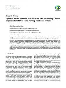
to force the output At) to track a given desired trajectory AA. This control structure was uroDosed in Reference 10 and it is called the globally l;ne&sing control structure; see Fig. 1.
If L,h(x) = 0 and the relative degree is r = 2, the second derivative of the output f i t ) is given by j;
= L;
h(x)
+ L, L, h(x)u
where Fig. 1
In general, the nonlinear system of eqn. 2 is said to have relative degree r if L,L)h(x)=O
i=O,
Y = h(x) j = L, h(x) j; = L; h(x)
... = LY-
Dynamic recurrent neural network
3
with Lyh(x) = h(x). An important case occurs when the relative degree r is equal to the number of states (r = n). The output and its derivatives can be written as
y'"' = L; h(x)
The design procedure using the GLC structure is simple: compute the linearising state feedback (eqn. 4) from the system model and then tune the PI controller (eqn. 6).
..., r - 2
L,Lj- "x) # 0
y(n-l)
Globally linearising control (GLC)structure
h(x) + L, L;- 'h(x)u
I
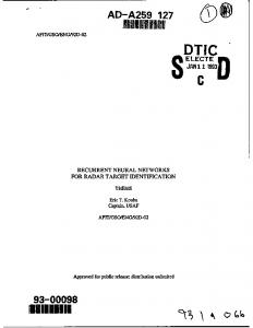
ANNs consist of many interconnected simple nonlinear systems called neurons. Generally speaking, neuron models can be divided in two basic types, static and dynamic. A dynamic neuron is the one whose output is described by a differential equation (see Fig. 2). A DRNN
(3)
2.2 Input-output linearisation The goal of the input-output linearisation technique is to cancel the nonlinear terms of the plant, using a state feedback, in order to have a linear dynamics between a new input v(t) and the actual plant output fit). If the input U for the system described by eqns. 3 is defined as
a
{U - LYh(x) - B,L;-'h(X)
(4)
1
then the last equation of eqns. 3 becomes, y'"' = U - /31L;- 'h(x) -
' '
- /3-
1L, h(x) -
8. h(x)
i.e. + ply(n-l) +
. .. + 8 , - 2 j i + 8 . - I j , + B , Y = ~
(I
(5)
The nonlinear terms L,L;- 'h(x), L;h(x) have been cancelled by the state feedback (eqn. 4) and the resulting system is linear between the new input U and the output y. The parameters bl, . .., 8. are based on the desired input-output characteristic; this means that the U - y system can have arbitrarily placed poles. 2.3 Globally linearising control
After linearising the system defined by eqns. 2 with the state feedback (eqn. 4),one can use an external PI loop = k,{r(t)
308
- fit))
+ ki
sb'
{r(t) - W) dt
1,........
A XI
b
Fig. 2 y(n)
........
xt4
(6)
Dynamic neuron model
The neuron is depicted in detail; note the differential equation for the output xi N
t = - x i + E~,,4(Xd+ Y,U 1-
*
b This simplifiedpicture is used as the building block for a dynamic network
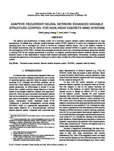
is a network of dynamic neurons with forward and backward connections (see Fig. 3). In this section it is demonstrated that a DRNN can approximate control affine systems of the class (2). Theorem 1 ; The dynamic recurrent neural network = -Tx
+ WU(,Y)+ Tu
(7) T e B N x N ,W e R N " , r f R N X 1 and 4x1 = {u((xl), . .., u(,Y,} can approximate the nonlinear
where
XE",
IEE Proc.-Control Theory Appl., Vol. 142, No. 4, July
Iws
This can be written as
system (eqn. 2) i=f(x)
x = - T X + WO(X)+ r u
+ gu
Y = h(x) The number of units N
Y = h(x) where
> n.
(14) and u((x)= u(xN)}. The total number of neurons is
X E % ~ ,T e ! R N x N ,
(u(x1),
...,
N=Nl+n. The network (eqn. 13) with T = I and no restrictions on the weight matrix W is known as the generalised Hopfield network and was first proposed by Hopfield [IS] in the context of associative memories. This network is described by
i = --x+wu(x)+ru Y = h(x) where X E %
4x1 = {'((xl),
Y
Fig. 3
Dynamic recurrent neural network ( D R N N )
Proof: The nonlinear system (eqns. 2) can be written as
+ gu
Y = 4x1
f0(x) = AX +f ( x ) A E %" " It is now well known that feedforward neural networks with one hidden layer can approximate any nonlinear function with arbitrary degree of accuracy [11-131; in Reference 14 it is stated that a feedforward neural network can be used to approximate the mappingf,(x)
+
In Section 2 it was shown that the relative degree is a key concept in order to linearise systems of the class (eqn. 2). In the following, it is demonstrated that a DRNN has the capacity to identify not only the dynamics of systems (eqn. 2) but also their relative degree. There are several patterns to obtain any relative degree with the dynamic neural network (eqn. 15); in this paper one of them is shown [9] when y i = 0, Vi # r. Theorem 2: The recurrent neural network
(9)
where C E W x N 1D,E ! R N l x n 0, E XN1and u ( x ) = {u(xl), ..., u(xN1)}.NI is the number of hidden neurons in the feedforward network. Substituting eqn. 9 in eqn. 8
where N
.f 2, if yi = 0, Vi # r and oij= 0, i = 1 , ..., r - 2 ; j = i 2, ..., N
+
The case when the relative degree is infinite is not considered. This situation occurs when the input does not affect the output, i.e. the system is autonomous. Proof: The proof of this theorem is illustrated by way of an example. Consider the following four-state (i = 1, 2, 3, 4) neural network 4
xi
Y = h(x) IEE Proc.-Control Theory Appl., Vol. 142, No. 4, July 1995
(17)
h(x) = X I
Define the new variable ( and its derivative (=Dx+e
r e x N x and 1
q(xN)}.
Relative degree of the DRNN
4
where
f0(x) = CO(DX 0)
rexNxN,
~ , ' ' '>
The computer simulations have shown that the model of eqn. 15 is more general than eqn. 13 and also the learning is faster. In this paper the identification and control of nonlinear systems is carried out using the model of eqn. 15.
=x,
i = -AX +f0(x)
(15)
=
--xi
+
wiju(xjX3 j= 1
+ yiu
Y =4 x ) =XI 309
In this model 4
&)
=
-xi + j 1 wij dxj) = 1
Pdx) = Yi Recall the mathematical definition of relative degree (Section 2.1): (i) Condition: y 1 # 0, y 2 = 0, y 3 = 0, y4 = 0 L,/;(x)= Y1 LpI;(x)# 0. Then r
(ii) Condition: y ,
=
1.
= 0, y 2
feedback (eqn. 4)that cancels the nonlinear terms of the plant; and (b) to obverve in open loop the plant and generate the state vector x needed in the linearising feedback. Then it is important to determine if the network as an open loop observer is stable, so the linearising feedback will work properly. The stability of the DNRR can be examined with the first method of Liapunov; in this method each equilibrium state is investigated separately. From eqn. 15, the autonomous dynamic network is,
li = - 2 + W 4 x ) (18) where x = Cxl, . . ., xNIT, W E S N x N ~ ( ,x =) C4xl),. . ., 4xN)IT.One equilibrium point ,y* is the solution of x* = Wu(x*)
# 0, y 3 = 0, y4 = 0
Expanding the right-hand side of eqn. 18 in Taylor series about the equilibrium state x* and deleting the higherorder derivatives, we obtain i=[ - I +H]z (19) with
4 L 3 1 ; ( x )# 0 if w12 # 0. Then r = 2. (iii) Condition: y1 = 0, y2 = 0, y 3 # 0, y4 = 0: L3
L,L,I;(x)
= w13 =
L f W = { -1
u’(X3)Y3
ifw13= o
o
+ wi i ~ ’ ( x i ) } f i ( x )
+ 0 1 2 U ’ ( x 2 ) f 2 ( x ) + w14‘‘(x4)f44(x) LpLjYx) = Ol2a’(X2)w23~’(x3)Y3
+ w14 u’(X4)w43
u‘(x3)Y3
L, Lf h(x) # 0. Then r = 3.
(iv) Condition: y1 = 0, y 2 = 0, y 3 = 0, y4 # 0, ~ Lf h(x) = { -
=3 0
+ 0 1 lU‘(x1)b14 O ’ ( x 4 h 4
+ O 1 2 u’0!2)w24
+
1
u’0!4)Y4
14 u’(x4)044 U‘(X4)?4
L ~ L ; I ; ( ~ )= o if col, = 0 w24 = o
We can write eqn. 19 as
i = Az where A=-I+H hll
Lq4x) = w l l u ” ( x l ) f 3 x ) + {-
1 + ~ll~’(x1)12fl(x)
+ { - 1 + % ~ ’ ( X l ) J ~ 1 2a ’ ( x 2 ) f 2 ( x ) + 0 1 2 4xz)w214xl)fl(x)
LpLqh(x)
+ w12 4 x 2 ) 0 2 2
O’(X2)f2(X)
+ w12 ‘ f ( x 2 b 2 3
u’(x3)f3(1()
= w12‘’(x2)023
u’(x3)w34‘’(x4)
LpL;h(x)# 0. Then r = 4. Finally, it is concluded that: r = 1 for y1 # 0, y 2 = 0, y 3 = 0, y4 = 0 r = 2 for y1 = 0, y 2 # 0, y 3 = 0, y4 = 0 and w12 # 0 r = 3 for y1 = 0, y 2 = 0, y 3 # 0, y4 = 0 and o13 =0 r = 4 for y1 = 0, y 2 = 0, y 3 = 0, y4 # 0 and w13= 0, w14 = 0, w24 = 0. 5
Stability of the DRNN
A
[
hii - 1
310
...
hNl
h:N hNN
]
-1
h.. = w ‘J. . gJ . ‘J i = l , ..., N j = 1 , ..., N Lyapunov showed that, if all the eigenvalues of the matrix A in eqn. 20 have nonzero real parts, then the stability of the equilibrium point x* of the original system (eqn. 18), is the same as that of the equilibrium point z = 0 of the linearised equation (eqn.20). It is possible to establish bounds for the real part of the eigenvalues of the matrix (eqn. 21) using the matrix measure [16]. 5.1 Matrix measure
A normed linear space is an ordered pair (X,11 ‘11) where X is a linear vector space and 11 : X -+ill is a real valued function called the norm. The concept of norm can be extended to include matrices IlAxII llAlli = SUP X#O
After the dynamic network has been trained, the model is used in two ways: (a) to calculate the linearising state
...
-1
llxll
this is called the induced matrix norm of A corresponding to the vector norm 11 . 11. I E E Proc.-Control Theory Appl., Vol. 142, No. 4 , July 1995
The matrix measure A A ) of a matrix A is the directional derivative of the induced norm I( . I l i at the point I (identity matrix), in the direction of A. That is
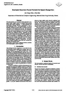
6.1 The plant The nonlinear plant is a single-link manipulator, shown schematically in Fig. 4. This plant is described by the
+
1 1 1 &Alli- 1
p(A) = lim e-o+
training, the network is tested for stability and for generalisation with other inputs.
&
There is one interesting property of the matrix measure [161 ; if l i is an eigenvalue of A, then - p ( - A ) < Re lid d.4) for asymptotic stability p(A) < 0 and d - A ) > 0. In this section two matrix measures corresponding to the I', I" norms in W are used to find the bounds for the real part of the eigenvalues for the linearised neural network, r
1
5.1.1 Stability from p, ;Calculating pl for eqn. 21
[
1 I +1 1 1
pl(A) = max h j j - 1 j
pl(-,4) = max j
+ 1 1 hijl ifj
1 - hjj
IhijI
(23)
if j
For asymptotic stability eqn. 22 must be negative
[
max h j j - l + C l h i j l j
mg
l I h i j I vj
(24)
i#j
note that if eqn. 24 is true then eqn. 23 is automatically satisfied.
5.12 Stability from p - : The same procedure is repeated for the matrix measure p m . The condition for asymptotic stability is -
1) >
1 I hijI
jfi
Vi
(25)
The conditions defined by eqn. 24 and eqn. 25 are sufficient and agree with those derived in Reference 17 using an eigenvalue localisation theorem known as the Gerschgorin's circle theorem. It is important to mention that the matrix measure states bounds and in particular the upper bound for the real part of the eigenvalues can be positive; this does not imply that the actual real part of the eigenvalues is positive. In other words the conditions of eqns. 24 and 25 are sufficient but not necessary.
6
+ U&) + mgl sin e(t) = u(t)
where the length, mass and friction coefficients are I = 1 m, m = 2.0 kg and U = 1.0 kg m2/s, respectively
and finally
-(hii
Single-link mnnipulaor
Wl.
The corresponding state representation is i' = x2 i 2= -9.8 sin x1 - 0 . 5 ~ 0~. 5 ~
+ (26) Y = XI with q ( 0 ) = x,(O) = 0 and y = qt). The plant (eqn. 26) was identified with the neural network (eqn. 16 and 17); the identification scheme assumes that the plant is a black box and the only available information is the input-output data. Fig. 5 shows nonlinear
state : X r R"
DRNN
Identification
It was shown in theorem 1 that the DRNN (eqn. 16) can approximate control affine systems of the class (eqn. 2). To illustate this result, a single-link manipulator is identified with a DRNN using random noise as the input. After I E E Proc-Control Theory Appl., Vol. 142,No.4, July I995
Y
-. plant
x
siaie : E R"
Fig. 5
Plant identification using the DRNN 311
the nonlinear plant and the dynamic neural network during the identification process.
Fig. 7 shows the output of the plant and the output of the network for the input (eqn. 28); the performance index was J = 0.0069.
6.2 Training The DRNN (eqns. 16 and 17) was trained with N = 5 neurons and a(x) = tanh (x) to identify the nonlinear plant (eqn. 26); the training was carried out repetitively over the fixed time interval [0, tJ] with the chemotaxis algorithm [19] to minimise the performance index (eqn. 27). The training input was random noise and the initial conditions for the neuron states were selected at random, tJ = 20 s. J
=
{$
=
[ir { y ( t ) - yn(t)}’ dt]’” tJ
0.4 03 02
,
0 1
0 -0 1 -0 2 -0 3 -0.41
c e 2 ( t )dt}’”
Fig. 7
Plant output and network output for the input of eqn. 28
0
Fig. 6 shows the output of the plant and the output of the neural network for the training input; the performance index after the training was J = 0.0064.
The stability of the trained network was tested using the first method of Liapunov and the matrix measure p w . The real part of the eigenvalues of the linearised network lies in the interval -5.8919
0.4-
< Re Ai < 4.0203
and the exact eigenvalues are -0.2260
+j3.1483
-0.2260 - j3.1483 -2.0288
+ j0.1798
-2.0288 - j0.1798 -0.4 1 Fig. 6
The parameters of the network after the training were as listed in Table 1. Table 1 : Network Daramaters after training Weiaht matrix W 0.4684 -2.4995 1.3615 0.0642 -0.8185 -0.9241 -0.3257 1.2319 -1.2444 0.4396 Weight vector -0.0050 -0.21 11 0.1 689 0.0645 -0.041 3
r
0.4211 0.0413 -0.0743 -1.0997 -0.5466
-0.2848 0.1 995 -1.8925 -1.6608 -0,1264 0.1484 0.2192 -0.8547 1.7342 -0.5953
Initial conditions -0.0097 -0.0065 0.0171 -0.0097 0.0025
The first component of the weight vector r is y1 z 0; then according to the relative-degree theorem, the trained network has r = 2, It can be seen that this is the same relative degree as that of the plant, so the network is capable to identify the dynamics of the plant and its relative degree. To verify the generalisation of the neural-network model, different inputs were used. One such input, is a sine wave
312
-0.4082
V
Plant output and network output for the training input
It is concluded that the trained network has good generalisation capabilities and it is stable, so it can be used as an open-loop observer. 7
Control
In this section the DRNN is used to cancel the nonlinear terms of the plant and to produce a desired linear dynamics between the new input U and the plant output y. Then the linearised plant is immersed in the GLC structure and a PI controller is adjusted to match a closed-loop desired response. The desired dynamics for the linearised plant was chosen as
liU
1
(sz
+ 5s + 6)
This is equivalent to the differential equation
3+
dY + 6y = U 5dt
The trained neural network was used to calculate the linearising state feedback
- L; 9 x 1 - B l Ll4X) - 8 2 9 x 1 (30) L, LI 4 x 1 where = 5 and B2 = 6. Fig. 8 illustrates the linearisation of the plant (eqn. 26) with the input (eqn. 30), and Fig. 9 compares the desired open-loop dynamics (eqn. 29) and the linearised plant dynamics for a random noise input v ; the performance index was J = 0.0187. Now the linearised plant is introduced into the GLC structure; the aim here is to ensure that the overall U =
U
IEE Proc.-Control Theory Appl., Vol. 142, No. 4, July 1995
closed-loop system matches some desired global dynamics. In this instance, a well damped second-order dynamics of the form
Fig. 12 shows the response for the step r = 0.5, when the mass of the single link manipulator was changed from 2.0 kg to 2.5 kg; the performance index was J = 0.0326. Fig. 13 presents the response for the step r = 0.5, when a 0.5 0.4T
A
0.2 0.1
0 -0.1
- 0.2 -0.31 Fig. 11 Desired closed-loopresponse and actual GLC responsefor the input of eqn. 32 U
lnput-output linearisation using the DRNN
Fig. 8
"1 0.2
i/.
Fig. 12 Desired closed-loop response and GLC responsefor a step re/erence r = 0.5 when the mass of the plant is changed from 2.0 kg to 2.5 kg
-0.21 Fig. 9 Desired open-loop dynamics and actual input-output plant dynamicsfor a random input U
-
was selected. The PI controller is v=
[p' +
:]e
where k , = 1.0 and ki is adjusted. Fig. 10 shows the desired closed-loop dynamics (eqn. 31) and the actual dynamics of the GLC structure for the
~
/+----
0.2 0.1
0 Fig. 13 Desired closed-loop response and GLC responsefor a step re/erence r = 0.5 when a disturbance of magnitude 0.1 is applied during the interual [lO.O, 12.01 s
disturbance of magnitude 0.1 was applied to the reference during the interval At = clO.0, 12.01 s; the performance index was J = 0.0132. 8
Fig. 10 Desired closed-loop response and actual GLC response for a step reference r = 0.5
reference input r = 0.5, the performance index (eqn. 27) [replacing y,(t) by yAt)] was J = 0.0121 with ki = 3.8. Fig. 11 shows the desired output and the plant output for the sinusoidal input (eqn. 32); the performance index was J = 0.0216.
Conclusions
It has been shown that the dynamic neural network (eqn. 15) can identify the relative degree and the dynamics of nonlinear systems of the class (eqn. 2). After training, the neural network can be used to synthetise a linearising state feedback that cancels the nonlinear terms of the plant and yields any desired linear dynamics U - y. The identified network is used in two ways: (a) to calculate the Lie derivatives of the linearising feedback (b) to generate, on-line, the state vector x needed in the Lie derivatives.
To cancel the nonlinear terms properly, the trained network must be stable. It was shown that, owing to the I E E Proc.-Control Theory Appl., Vol. 142, No. 4, July I995
313
7 KRAVARIS, C., and KANTOR, J.C.: ‘Geometric methods for nonparticular structure of the proposed DRNN, the stability linear P r m S control: 1. Background: Ind. EW. chm.Res., 1994 ~ pp. ~ 2295-2310 can & tested easily using the first method of ~ i ~ p u n 29, and a matrix measure. 8 KAMBHAMPATI, C., MANCHANDA, S., DELGADO, A., Finally. the simulation results showed that the perGREEN. G.G.R.. WARWICK, K., and THAM, M.T.: ‘On the relative order inverses and the architecture of a class of recurrent formance of the GLC structure is satisfactory and robust. networks’, Automatica (to be published) For example, the network was trained with a payload of 9 DELGAW, A.: ‘Differential geometric control of nonlinear systems 2.0 kg and the system was tested with a payload of with recurrent neural networks’. Internal research report of the 2.5 kg; it can be seen that the resulting response does not Cybernetics Department, Reading University, 1994 IO KRAVARIS, C., and CHUNG, C.B.: ‘Nonlinear state feedback synvary significantly. At the same time, it can be seen that thesis by global input/output linearization’, AlChE J., 1987, 33, innuts in the form of unmeasurable disturbances do not effect the performance. In fact with disturbance the index 11 G,: ‘Approximation by superpositions of a sigmoidal value is J = 0.0132 while without the disturbance it is functionv. Techniral report, University of Illinois Urbana-
!!!::;FA,
J
= 0.0121.
Champaign Department of Electrical and Computer Engineering,
In general, if the DRNN is trained properly and it is stable with good generalisation capabilities, it can be used as an Observer for systems Of the ‘lass defined by eqn. 2.
1988 12 HORNIK, K.: ‘Multilayer feedforward networks are universal approximators’, Neural Networks, 1989.2, pp. 359-366 13 FUNAHASHI, K.I.: ‘On the approximate realization of continuous mappings by neural networks’, Neural Networks, 1989, 2, pp. 183192
References
9
1 MILLER 111, W.T., SUTTON, R.S., and WERBOS, P.J.: ‘Neural networks for control’ (MIT Press, 1992) 2 HUNT, KJ., SBARBARO, D., ZBIKOWSKI, R., and GAWTHROP, P.J.: ’Neural networks for control systems - a survey’, Automtica, 1992, 28, pp. 1083-1112 3 CHEN, S., and BILLINGS, S.A.: ‘Neural networks for nonlinear dynamic system modelling and identification’, Int. J. Control, 1992, 56, pp. 319-346 4 NARENDRA, K.S.,and PARTHASARATHY, K.: ‘Identification and control of dynamical systems using neural networks’, IEEE Trans., 1990, ”-1, pp. 4-26 5 PAO, Y., PHILLIPS, S.M., and SOBAJIC, D.J.: ‘Neural net comnutinn and the intelligent control of systems’. . Int. J . Control. 1992. pi. 263-289 6 ISIWRI, A.: ‘Nonlinear control systems’ (Springer-Veda& 1989)
k,
314
-
14 FUNAHASHI, K.I.: ‘Approximation of dynamical systems by continuous time recurrent neural networks’, Neural Networks, 1993, 6, pp. 801-806 15 HOPFIELD, JJ.: ‘Neurons with graded response have collective computational properties like those of two state neurons’, Proc. Natl. Acad. Sei. USA, 1984.81, pp, 3088-3092 16 VIDYASAGAR, M.: ‘Nonlinear systems analysis’ (Prentice-Hall, New Jersey, 1993) 18 17 PERFEITI, R.: ‘Asymptotic stability of equilibrium points in dynamical neural networks’, IEE Proc. D, 1993,140, pp. 401-405
JIN, L., NIKIFORUK, P.N., and GUPTA M.: ‘Direct adaptive output tracking control using multilayered neural networks’, IEE Proc. D, 1993,140, pp. 393-398 19 BREMERMANN, H.J., and ANDERSON, R.W.: ‘An alternative to back propagation : a simple rule of synaptic modification for neural net training and memory’. Report PAM-483, Center for Pure and Applied Mathematics, University of California, Berkeley, 1990
IEE Proc.-Control Theory Appl., Vol. 142, No. 4 , July 1595