IEEE TRANSACTIONS ON SIGNAL PROCESSING, VOL. 62, NO. 9, MAY 1, 2014
2345
Adaptive Double Subspace Signal Detection in Gaussian Background—Part I: Homogeneous Environments Weijian Liu, Wenchong Xie, Jun Liu, Member, IEEE, and Yongliang Wang, Member, IEEE
Abstract—In this two-part paper, we consider the problem of adaptive multidimensional/multichannel signal detection in Gaussian noise with unknown covariance matrix. The test data (primary data) is assumed as a collection of sample vectors, arranged as the columns of a rectangular data array. The rows and columns of the signal matrix are both assumed to lie in known subspaces, but with unknown coordinates. Due to this feature of the signal structure, we name this kind of signal as the double subspace signal. Part I of this paper focuses on the adaptive detection in homogeneous environments, while Part II deals with the adaptive detection in partially homogeneous environments. Precisely, in this part, we derive the generalized likelihood ratio test (GLRT), Rao test, Wald test, as well as their two-step variations, in homogeneous environments. Three types of spectral norm tests (SNTs) are also introduced. All these detectors are shown to possess the constant false alarm rate (CFAR) property. Moreover, we discuss the differences between them and show how they work. Another contribution is that we investigate various special cases of these detectors. Remarkably, some of them are well-known existing detectors, while some others are still new. At the stage of performance evaluation, conducted by Monte Carlo simulations, both matched and mismatched signals are dealt with. For each case, more than one scenario is considered.
TABLE I THE MAIN SYMBOLS USED IN THIS PAPER
Index Terms—Constant false alarm rate (CFAR), double subspace signal, generalized cosine-squared, homogeneous environments, multidimensional signal, signal mismatch.
NOTATIONS: Throughout the two-part paper lightfaced lowercase letters denote scalars, boldfaced lowercase letters stand for vectors, and boldfaced uppercase letters represent ma, , and denote trices. For a complex matrix , , the conjugate, transpose, conjugate transpose, and vectorizais the orthogonal projection matrix tion of , respectively. . onto the column subspace of , i.e., . For a square matrix , , Moreover, , and stand for the trace, determinant, and Frobenius Manuscript received July 19, 2013; revised December 04, 2013; accepted February 19, 2014. Date of publication March 05, 2014; date of current version April 07, 2014. The associate editor coordinating the review of this manuscript and approving it for publication was Prof. Maria Sabrina Greco. This work was supported in part by National Natural Science Foundation of China (No. 61102169 and 60925005). W. Liu is with College of Electronic Science and Engineering, National University of Defense Technology, Changsha 410073, China (e-mail: liuvjian@ 163.com). W. Xie and Y. Wang are with Wuhan Radar Academy, Wuhan 430019, China (e-mail:
[email protected];
[email protected]). J. Liu is with the National Laboratory of Radar Signal Processing, Xidian University, Xi’an 710071, China (e-mail:
[email protected]). Color versions of one or more of the figures in this paper are available online at http://ieeexplore.ieee.org. Digital Object Identifier 10.1109/TSP.2014.2309556
norm of , respectively. For a positive definite matrix , , , and stand for the square-root matrix, inverse of the square-root matrix, and the maximum nonzero eigenvalue of , respectively. For a scalar function of a vector or matrix , , and denote the partial derivative argument , of with respect to (w.r.t.) , the natural logarithm of , and the statistical expectation of w.r.t. , respectively. Furthermore, denotes the maximum likelihood estimate of under hypoth, 2. Moreover, denotes the Kronecker product, esis , means the minimum value of and , and is the identity matrix of order . In addition, we summarize the main symbols used in this paper in Table I for ease of reference.
T
I. INTRODUCTION
HE problem of adaptive detection of a multidimensional/multichannel signal in Gaussian or non-Gaussian noise with unknown statistical property has received an increasing attention for more than two decades. For a large number of these detection problems, the basic form of the
1053-587X © 2014 IEEE. Personal use is permitted, but republication/redistribution requires IEEE permission. See http://www.ieee.org/publications_standards/publications/rights/index.html for more information.
2346
IEEE TRANSACTIONS ON SIGNAL PROCESSING, VOL. 62, NO. 9, MAY 1, 2014
signal is usually known a priori, whereas the covariance matrix of the noise is unknown. This essentially necessitates the use of adaptive methods. In particular, a set of training samples (secondary data) is required. Each training sample contains only noise and shares the same covariance matrix (homogeneous environments) or up to an unknown scaling factor (partially homogeneous environments) with the test data (primary data). For the problem at hand, there are three common design criteria, namely, the generalized likelihood ratio test (GLRT), Rao test, and Wald test. Moreover, their two-step variations are usually adopted in practice. Based on these design criteria, a large number of detectors are proposed under various settings. In particular, in [1] it is assumed that the echoes from the distributed target are all reflected in the same direction but with different power levels. According to the GLRT design criterion, the so-called multiband generalized likelihood ratio (MBGLR) test is proposed. The model in [1] is also adopted in [2], [3]. Precisely, several GLRT-based detectors are proposed in [2], while the Rao and Wald tests, and their two-step versions, are exploited in [3]. When the signature of the signal is completely unknown, three GLRT-based detectors and a type of spectral norm test (SNT) are proposed in [4]. The assumption of the availability of secondary data has been removed in [5], and a modified GLRT (MGLRT) is derived. This idea is generalized in [6], [7] by adding different types of interference. Most detectors mentioned above are devised on the assumption of homogeneous environments. A common class of nonhomogeneity is partial homogeneity. That is to say, the covariance matrices of the primary and secondary data share the same structure but with different power levels [8]. The detection problems in this situation are explored in [2], [8]–[10]. A milestone in the field of multichannel adaptive detection is the report by Kelly and Forsythe [11], whose model is very general and contains many kinds of point targets and distributed targets as its special cases. Precisely, the problem of adaptive detection in [11] is equivalent to making a decision between the following two hypotheses (1) -dimensional primary data and stands where is the for the noise matrix of the same dimension. Whenever we speak of the term noise, we always mean noise in a broad sense, which may include clutter, jamming, and thermal noise. Each column of is modeled as an independent and identically distributed (IID), zero-mean, complex circular Gaussian random vector with an unknown positive definite covariance matrix . and are two known matrices, describing the signal structure, while is the unknown coordinate, denoting the signal amplitude parameter. The dimensions of , , and are , , and , respectively. Moreover, and are full-column-rank and full-row-rank, respectively. Note that the signal model in (1) can be obtained by multichannel acquisition [such as sensor array and multiple-input multiple-output (MIMO) radar] or/and multidimensionnal acquisition (e.g.,
multiple range bins and Doppler bins for radar systems). Note that no secondary data set is employed in [11]. However, an . This important assumption is the constraint important assumption ensures the existence of an equivalent secondary data set, conducted by a certain unitary matrix transformation to the primary data . The equivalent secondary data set can form a nonsingular SCM with probability 1; refer to [11] for details. According to the GLRT design criterion, the detection problem in (1) is investigated extensively in [11] under the assumption of homogeneous environments. In this paper, we move a further step towards the design and analysis of adaptive detectors. The main contributions of this part of the paper lie in the following four aspects. First, we generalize the model of [11]. We do this by abandoning the constraint and assume a set of secondary data is available, which contains no signal component and shares the same covariance matrix with the primary data. It seems no significant difference between the data model above and that adopted in [11]. Nevertheless, the rows of the signal matrix in [11], after the unitary transformation, lie in the entire space. In other words, the structure of the row space of the signal after the unitary transformation is lost. Essentially, the signal model . employed in [11] is equivalent to ours only when Second, we derive the GLRT, Rao test, and Wald test, as well as their two-step versions, and introduce three SNTs. All these detectors are shown to ensure the constant false alarm rate (CFAR) property. We also show the differences between them and how they work. Third, we show many special cases of the novel detectors. Some are found to be the existing detectors, whereas the others are still new. Finally, we investigate the detection performance of these detectors both for deterministic and random signals. Moreover, we also investigate the detection problem when signal mismatch exists. The rest of this part is organized as follows. Section II deals with the problem formulation and gives some important special cases about the data model, while Section III presents the detectors, gives their differences, and shows how they work. Various special cases of the detectors are exploited in Section IV. The performance evaluation, conducted by Monte Carlo simulations, is addressed in Section V. Finally, Section VI concludes this part of the paper. II. PROBLEM FORMULATION As stated above, the model of (1) is generalized in the following binary hypothesis test: , ,
(2)
where , , , , and are mentioned above. stands for the noise in the -dimensional secondary data . Each column of has the same statistical properties as the noise matrix . It is worth noting that the model in (2) is well known as the generalized multivariate analysis of variance (GMANOVA) in the field of multivariate statistics [12].
LIU et al.: PART I: HOMOGENEOUS ENVIRONMENTS
2347
III. THE DETECTOR DESIGN AND ANALYSIS
It is also noteworthy that the signal model can be recast as (3) is the th column of , is the th row of , and where is the th component of . Equation (3) gives some geometrical interpretation about the matrices , , and . Precisely, and span the column subspace and row subspace (i.e., the signal structure) where the signal lies in, while stands for the corresponding coordinate (i.e., the amplitude parameter). For convenience, we call a signal a double subspace signal, if it has a form shown in (3). It is noteworthy that when collapses to a scalar, taking the vectorization operation of both sides of (3) results in the steering vector for space-time adaptive processing (STAP) for airborne radar [13]. The data model in (2) is of considerable flexibility. In the following, we present some important special cases. • Case 1. and . Consequently, both and reduce to scalars, absorbed into a single scalar. Moreover, reduces to a column vector, which is usually called the steering vector in this scenario. The corresponding detection problem is exploited extensively in [14]–[42]. • Case 2. , , and . In this case, collapses to a scalar and turns into a column vector. The detection problem under this scenario is addressed in [36], [43]–[52]. A special subcase is , which is equivalent to the case that no information about the column space of the signal is available. The corresponding GLRT in exploited in [53]. • Case 3. , , and . Consequently, , , and turn into a column vector, a row vector, and a square matrix, respectively. Without loss of generality, we can set , since is known a priori. The problem of adaptive detection under this setting is investigated detailed in [1]–[3], [5], [7], [9], [10], [42], [54]–[59]. • Case 4. , , and . As explained above, this case is equivalent to the model adopted in [11], where the detection problem based on the GLRT is analyzed detailedly. Another example is [60], where, besides the signal, a certain subspace interference exists. Moreover, a special case is . Hence, we can set . That is to say, no structure information about the signal is known in advance. The corresponding detection problem is explored in [4], [61]. • Case 5. , , , , and , , and/or has a special structure. Subcase 1) is a diagonal matrix. An example of this subcase is the colocated MIMO radar detection for multiple targets [62]. Subcase 2) and are both diagonal or block-diagonal matrices. An example for the former case is the distributed MIMO radar detection in [63] [after performing matched filtering to (11) therein], while an example for the latter case is [64], where the detection and estimation problem is investigated in the context of MIMO radar with multiple transmitting and receiving subarrays. Note that it does not resort to secondary data in [62]–[64].
A. Design of the Detectors The one-step GLRT, or simply GLRT, is tantamount to maximizing the likelihood ratio over all the unknown parameters [14], written symbolically as
(4)
where is the joint probability density function (PDF) of and under hypotheses , , 2. Let be the parameter vector partitioned as (5) where and . Then the Rao and Wald tests for complex-valued signals are given below [65]
(6)
(7) where
is the FIM, defined as [65]
(8) which can be partitioned in the following manner (9)
The term
in (6) and (7) is calculated as follows:
(10) is the value of under hypothesis . Moreover, Besides the GLRT, Rao test, and Wald test, their two-step variations are also usually employed in practice and have the following two steps. First, it is assumed that the noise covariance matrix or only its structure is known and the corresponding detector is derived based on the primary data. Then, the unknown noise covariance matrix or its structure is replaced by a proper estimate [2], [15].
2348
IEEE TRANSACTIONS ON SIGNAL PROCESSING, VOL. 62, NO. 9, MAY 1, 2014
For the detection problem in (2), the GLRT, Rao test, Wald test, and their two-step versions are given below1 (see Appendix A)
(11)
(12) (13) (14) where
,
,
,
,
Remark 1: The AOD has an upper bound on detection performance for the other detectors, owing to the assumption of known . Remark 2: From the expressions of the detectors, one can see that an important step is the estimation of the covariance matrix . Moreover, the covariance matrix estimates for the Rao test, Wald test, and the 2SD are different. Notably, it seems that the Rao test, Wald test, and the 2SD can be obtained by replacing in the detection statistic of the AOD with the corresponding estimates. Remark 3: It seems that these detectors use different estimates of to whiten the primary data and the signal component . For the AOD, and are truly whitened [67], whereas they are quasi-whitened [57] for the other detectors in different manner. Remark 4: When the number of the secondary data is infinite, the GLRT, Rao test, Wald test, and the 2SD all approach the AOD. However, the three SNTs (see below) can never approach the AOD, unless or is of rank one, since the SNTs only take the maximum eigenvalues of the corresponding matrices.
(15) (16)
B. Some Further Interpretations of the Detectors In order to show how these detectors work, we rewrite the GLRT, Rao test, Wald test, and the 2SD as follows:
and (17) It is worth noting that two-step versions of the GLRT, Rao test, and Wald test coincide with each other, shown in (14), and are denoted as the two-step detector (2SD). Moreover, (12), (13), and (14), can be represented by the following compact forms (18) (19) (20) where
,
,
,
, , and . For comparison purpose, we derive a detector when the covariance matrix is known. From (58), (62), and (68) in Appendix A, we know that the GLRT, Rao test, and Wald test coincide with each other. For clarity, it is shown below: (21) where
,
, and
. For convenience, the detector in (21) is referred to as the asymptotic optimum detector (AOD) in homogeneous environments. 1In
this part of the two-part paper, we add the letter h in the subscript of each detector to indicate it is devised in homogeneous environments. This subscript is used to differ from the detectors in the Part II [66].
(22) (23) where
,
, and
. Note that the key parameters of the detectors are the three quantities , , and , or equivalently, , , and , where , , , is given in (16), and is given in (17). Remark 5: Post-multiplication of is tantamount to the ordinary coherent integration of the entries of in the row direction, while pre-multiplication of , , or , corresponds to adaptive whitening and coherent integration in the column direction. Obviously, the corresponding whitening, however, is carried out in three different ways. Note that the effect of and is also pointed out in [11]. Besides the GLRT, Rao test, Wald test, and their two-step versions, an ad hoc detector, named as the SNT, is first introduced in [4] to detect a distributed target with completely unknown signature. Based on the analysis above, we extend the idea of the SNT by introducing the following three variations: (24) (25) (26)
LIU et al.: PART I: HOMOGENEOUS ENVIRONMENTS
2349
From the expressions of the Rao test, Wald test, and the 2SD, these three detectors can be regarded as energy detectors. In contrast, the three SNTs behave more like direction detectors, which search for a preferred direction, namely, the direction of maximum energy; refer to [8], [68] for detailed analysis. The difference between the three SNTs is how the whitening is done. Obviously, this difference also holds for the Rao test, Wald test, and the 2SD. Remark 6: The Rao test, Wald test, SNT2, and SNT3 can even work in the sample-starved situation, namely, the case when the number of the secondary data is less than that of rows of the primary data, i.e., . Precisely, the Rao test and the SNT2 can work when the following constraint is satisfied: . For the Wald test and the SNT3, the constraint becomes . C. CFAR Property of the Detectors Due to its importance, the CFAR property has become a necessary condition for modern adaptive detector design [69]. In this subsection, all the proposed adaptive detectors are shown to be CFAR2. We first show the GLRT ensures the CFAR property. Note that the term in the numerator of (11) can be expressed as
According to the partitioned matrix inversion formula [73, p.363], along with the result , we can represent (28) by
(29) where
,
, , and . We have used the equality in (29). Since and are independent on under hypothesis , clearly from (27) and (29), the GLRT is also independent on under hypothesis . Hence, the CFAR property of the GLRT follows. Moreover, (12) and (13) can be rewritten as ,
(30) and
(27) where and . Obviously, each column of the matrix , under hypothesis , is distributed as a zero-mean complex circular Gaussian random vector, with a covariance matrix . Meanwhile, , under hypothesis , is ruled by an -dimensional complex central Wishart distribution with degrees of freedom (DOFs) and an associated co[72]. Hence, the term , under hypothvariance matrix esis , is independent on . Moreover, one can verify that the term in the denominator of (11) can be recast as
. Notice
is independent on , the denominator of (11) that if is also independent on . In fact, this is indeed the case. The quantity can be rewritten as
(28) where , , and is a unitary matrix , with . partitioned as is a semi-unitary matrix such that and . Note that is statistically equivalent to under hypothesis . So is w.r.t. . 2By CFAR, we mean that a detector, under hypothesis , is independent on the noise covariance matrix (i.e., both the noise level and the noise covariance matrix structure). This is denoted as matrix-CFAR in [70] and covariance-matrix-CFAR in [71].
(31) respectively, where and . Taking the same fashion as that of (29), we have the result that the Rao and Wald test are both CFAR. Clearly from the analysis above, the three SNTs are also CFAR. IV. SPECIAL CASES OF THE DETECTORS In this section, we show various special cases of the detectors, some of which are closely related with the existing ones. The special cases of the detectors can be roughly classified into the following three categories: 1) special case A: and , 2) special case B: and , and 3) special case C: and . Each category has several subcases. The main results are shown in Table II. For ease of reference, the general cases of the detectors are also given in Table II. We also add the reference(s) when a certain detector has been derived in previous literature according to the corresponding design criterion. Note that it is easy to obtain most special cases of the detectors from the corresponding general cases. Thus, the detailed derivations are omitted. Moreover, some special cases have more than one equivalent form, mainly for the GLRT, which is not included in Table II for brevity and will be given below. We first give some equivalent forms of the GLRT when and . In this case, the GLRT in (11) turns into (32) which is the GLRT exploited extensively in [11].
2350
IEEE TRANSACTIONS ON SIGNAL PROCESSING, VOL. 62, NO. 9, MAY 1, 2014
TABLE II THE DETECTORS AND THEIR SPECIAL CASES IN HOMOGENEOUS ENVIRONMENTS
Let . According to (A1–2) in [11], for any conformable matrices involved, we have the following result (33)
It is worth noting that the GLRT for the colocated MIMO radar addressed in [64] is essentially identical to (35) (see (31) in [64]). If , (32) becomes
Hence, (32) can be expressed as
(36) Further, (36) can be rewritten as (37)
(34) Moreover, it is shown in [11] that (32) can be recast as where (35)
, .
, and
LIU et al.: PART I: HOMOGENEOUS ENVIRONMENTS
2351
Equation (37) is equivalent to (38) which is exactly the GLRT in [1], [2]. Now we show some equivalent forms of the GLRT when and . In this scenario, . Thus the GLRT in (11) degenerates into (39) Using a special case of (33), we can represent (39) by the form shown in Table II in this particular case. Moreover, in light of (33), we can rewrite the numerator and denominator of (39) as (40) and Fig. 1. PD versus SNR for the deterministic-uniform signal model.
(41) respectively. Substituting (40) and (41) into (39) leads to (42) Applying (33) to the denominator of (42) yields
(43) Exploiting the matrix inversion lemma to the denominator of (43), we have (44) which is a dual version of (35). Note that when and , the Rao test is also derived according to a modified two-step GLRT (M2S-GLRT) in [4]. The SNT1 when is the maximum eigenvalue detector in [68] for a different detection problem from ours. It is also worth noting that under a certain special case, a detector can be obtained by different design criteria [74]. This can be seen from Table II. Some of these results are obvious, while the others are not straightforward. For the latter case, we show the corresponding derivations in Appendix B.
Fig. 2. PD versus SNR for the deterministic-dominant signal model.
V. PERFORMANCE EVALUATION For space limitations, we only consider the general case, i.e., and . We assess the detection performance of the detectors both for matched signals (Figs. 1–6) and for a type of generalized mismatched signals (Figs. 7–8). As for the former case we consider both deterministic and random signals, while for the latter case we only consider deterministic signals (for the sake of brevity). Deterministic signals correspond to a nonrandom coordinate matrix , while random signals correspond to the case that the components of are random. As for , deterministic or random, two subcases are exploited. One is that the norm of one column of is significantly larger than the sum of the norms of the other columns when , i.e.,
Fig. 3. PD versus SNR for the random-uniform signal model.
with
and
, where is partitioned as being the first one and last columns of
, .
2352
IEEE TRANSACTIONS ON SIGNAL PROCESSING, VOL. 62, NO. 9, MAY 1, 2014
Fig. 4. PD versus SNR for the random-dominant signal model.
Fig. 5. PD versus SNR for deterministic signals when is in a uniform or dominant form. The solid line stands for the case that is in a uniform form, while the dotted line denotes that is in a dominant form. The symbols , ☆, , o, , , and , stand for GLRT, Rao test, Wald test, 2SD, SNT1, SNT2, and SNT3, respectively.
The other case is that each column of has roughly the same norm. More precisely, we set for the former and for the latter, no matter whether is deterministic or random. The matrix is a semi-unitary matrix of dimension , i.e., . is an -dimensional diagonal matrix with the first diagonal element and the other diagonal elements (if ). One can tune the scalar to ensure certain signal-to-noise ratio (SNR), defined below. For convenience, when is in the form , we say is in a uniform form. In contrast, when is in the form , we say is in a dominant form. Moreover, when is deterministic and in a uniform form, we denote the signal model as a deterministic-uniform signal model. In a similar manner, when is deterministic and in a dominant form, we refer to the signal model as the deterministic-dominant signal model.
Fig. 6. PD versus SNR for random signals when is in a uniform or dominant form. The solid line stands for the case that is in a uniform form, while the dotted line denotes that is in a dominant form. The symbols , ☆, , o, , , and , stand for GLRT, Rao test, Wald test, 2SD, SNT1, SNT2, and SNT3, respectively.
Fig. 7. PD versus .
for the deterministic-uniform signal model.
The random-uniform and random-dominant signal models can be analogously defined. For deterministic signals, the SNR is defined as (45) When the signal is random, we model the th column of , say , as a zero-mean complex circular Gaussian vector, statistically independent on each other, and has the covariance matrix . Then, a reasonable SNR can be defined as [66] (46) The noise and the signal coordinate matrix , if the signal is random, are both modeled as exponentially correlated random vectors with one-lag correlation coefficient. That is to say, the th and th elements of and are given by
LIU et al.: PART I: HOMOGENEOUS ENVIRONMENTS
Fig. 8. PD versus .
2353
for the deterministic-dominant signal model.
and
, respectively, . We set , , and throughout this section. In order to reduce the computational complexity, the probability of false alarm (PFA) is set to be in all simulations. To evaluate the probabilities of detection (PDs) and the detection thresholds (necessary to ensure a prescribed PFA), we resort to and independent data realizations, respectively. Moreover, we set and in all simulations and use the GLRT as a benchmark through this section. Fig. 1 plots the PDs of the detectors for the deterministic-uniform signal model under different SNRs. A remarkable feature is that with the increase of , the PD of a certain detector decreases. In order to interpret this phenomenon, we take the vectorization operation of both sides of (3), which results in and
(47) where , , and . The dimensions of , , and are 1, , and 1, respectively. From (47), we see that the signal lies in the subspace spanned by the columns of . Note that corresponds to the completely known signal direction, while corresponds to the unknown signal direction. Hence, when and/or increases, the uncertainty of the signal direction also increases. This may result in certain performance loss. Moreover, when increases (other parameters are unchanged), the PD of a certain detector also increases. Note that the increase of results in the increase of the number of the rows of in (47), whereas the number of the columns of is unaltered. This is tantamount to reducing the uncertainty of the signal direction (see Figs. 3–4 for the effect of the change of the values of and on the detection performance). The results in Fig. 1 also indicate that, for the specific scenario, the GLRT, compared to the AOD, suffers a performance loss of about 4 dB in terms of SNR at . Obviously, when the number of the secondary data becomes large, this loss will decrease. On the other hand, the GLRT has a higher PD than the other adaptive detectors if the SNR is not very high. In contrast, when the SNR
is high enough, the Wald test provides a slightly higher PD than the GLRT. Moreover, the change of does not significantly affect the rank of the detectors. Note that the relationship between the GLRT and Wald test is very like that between Kelly’s GLRT [14] and the AMF [15] (which is also a Wald test [17]). Fig. 2 is analogous to Fig. 1, but it corresponds to deterministic-dominant signal model. When and , the hierarchy of the detectors is similar to that in Fig. 1. In contrast, when , , and , for the case of , the detection performance of the GLRT is inferior to the other detectors except for the Rao test. Moreover, in this case, the Rao test nearly turns invalid. A possible justification about the good performance of the SNTs is given below. The SNTs only choose the energy in a preferred direction. This has two effects and the latter one dominates the first one. The first one is the loss of the energy in other directions that tends to decrease detection performance. The other one is the mitigation of the perturbation, introduced by the covariance matrix estimates. The latter effect results in statistical stability, and hence improves detection performance. Note that similar explanations are given in [4] and [61]. Figs. 3 and 4 display the detection performance of the detectors for the random-uniform and random-dominant signal models, respectively. By comparing the results in Figs. 3 and 4, we see that for random signals, the detection performance of the detectors is dramatically affected by the fact that whether is in a uniform or dominant form. In the random-uniform signal model, the GLRT roughly has the highest PD, irrespective of the value of . Moreover, in the random-dominant signal model, when is small, the GLRT also has the highest PD. However, when is large, both the SNT2 and SNT3 have higher PDs than the GLRT. In fact, when and/or is large enough (not shown here for space limitations), even the 2SD and SNT1 have higher PDs than the GLRT. Figs. 5 and 6 show the property of that whether it is in a uniform or dominant form on the detection performance for deterministic and random signals, respectively. The results highlight that for deterministic signals, no matter whether is in a uniform or dominant form, it does not substantially affect the detection performance of a certain detector. In contrast, it does affect the detection performance for random signals. More precisely, for random signals there is roughly a 3 dB loss for a certain detector at when is in a dominant form, compared to the case of a uniform-form . The detection performance is characterized in a different way in Figs. 7 and 8, which illustrate the PDs of the detectors for mismatched signals. The phenomenon of signal mismatch often occurs due to imperfect array calibration, wavefront distortions, beampointing errors, etc. Due to space limitations, only deterministic signals are considered. In order to quantify the mismatch, we assume the actual signal is , where is not necessarily equal to . Define an inner product, denoted by , over as , where and are two arbitrary matrices in . Hence, the angle between and in the inner product space above can be defined as
(48)
2354
IEEE TRANSACTIONS ON SIGNAL PROCESSING, VOL. 62, NO. 9, MAY 1, 2014
which is denoted as the generalized cosine-squared (GCS) between and in the whitened space. The GCS in (48) is a generalization of the quantity used to quantify the signal mismatch for point-like targets [18], [27]. The results in Figs. 7–8 imply that the detectors can be sorted into three categories, i.e., robust detectors (the Wald test, 2SD, SNT1, and SNT3), selective detectors (the Rao test and SNT2), and compromised detectors (the GLRT), according to the capabilities of the mismatched signal rejection.
(51) where . Taking the derivative of (51) w.r.t. and equating the result to zero yields the MLE of under hypothesis (52) Plugging (52) into (51), we have
VI. CONCLUSIONS In this part of the paper, we have investigated the problem of adaptive detection of a double subspace signal in homogeneous environments. The model is a generalization of that in Kelly and Forsythe’s classic report. Seven effective detectors have been proposed, which can be classified into three types, i.e., the ratio of two determinants of matrices (the GLRT), the trace of matrices (the Rao test, Wald test, and 2SD), and the maximum eigenvalue of matrices (the three SNTs). All these detectors are CFAR and cover several existing detectors as their special cases. At the stage of performance analysis, we have considered four kinds of signal models, i.e., deterministic-uniform, deterministic-dominant, random-uniform, and random-dominant. It is shown that: • None of the proposed adaptive detectors is uniformly better than the others. • Roughly speaking, the GLRT has the highest PD in the following two scenarios. One is that is in a uniform form, no matter whether it is deterministic or random. The other is that is in a dominant form and the value of the product of is small w.r.t. the product of , no matter whether is deterministic or random. • When is in a dominant form and the value of the product of is moderately large w.r.t. the product of , the SNTs and Wald test have higher PDs than the GLRT. In contrast, the Rao test exhibits the lowest PD in this case. • In the situation of signal mismatch, no matter whether is in a uniform or dominant form, it does not significantly affect the detection performance of the detectors. Precisely, the Rao test and SNT2 have the best performance in terms of mismatched signal rejection, while the Wald test, 2SD, SNT1, and SNT3 are most robust. Moreover, the GLRT is in between. APPENDIX A THE DERIVATIONS OF THE GLRT, RAO TEST, WALD TEST, AS WELL AS THEIR TWO-STEP VERSIONS The GLRT: The joint PDF
Substituting (50) into (49) yields
is found to be
(49) where and is times the SCM. can be obtained by setting in (49). It is well-known that the maximum likelihood estimate (MLE) of for given , under hypothesis , is [14]3 (50) 3We add the subscript 1 or 0 to indicate the corresponding quantity is the MLE or . under hypothesis
(53) Setting in (51) yields . Taking the th root of the ratio of (53) and results in the GLRT, given in (11). The Rao Test: In light of (49), we have the following two identities (54) (55) Substituting (54) and (55) into (8) results in
(56) where in the second equality we have used and in the last equality we have employed , for any conformable matrices involved. In a similar fashion, one can verify that and are both null matrices of appropriate dimensions. As a consequence, we have (57) Plugging (54), (55), and (57) into (6), and setting , after some straightforward algebraic manipulations, yields the intermediate Rao test for given (58) It is easy to show that the MLE of , under hypothesis , is . Plugging it into (58) and dropping the constant scalar, yields the final Rao test, shown in (12). We find that applying the matrix inversion lemma, after some algebra, we can rewrite (12) as (59) where
LIU et al.: PART I: HOMOGENEOUS ENVIRONMENTS
The Wald Test: Since trix, along with (56), we have
2355
is found to be a null ma(60)
Taking the derivative of (49) w.r.t. and setting the result to zero yields the MLE of , with fixed, under hypothesis
APPENDIX B THE PROOF OF THE EQUIVALENCE OF SOME DETECTORS UNDER CERTAIN PARTICULAR CASES The Equivalence of the GLRT and the Rao Test When and : In this situation, the GLRT in (11) degenerates into (69)
(61)
while the Rao test in (12) collapses to
Inserting (61) and (60) into (7) results in the intermediate Wald test for given
(70) According to the matrix inversion lemma, we have
(62) In order to obtain the explicit Wald test, we need the MLE of under hypothesis . Inserting (61) into (49) results in
(71) It follows that (72) As a consequence, (69) can be recast as
(63) Taking the derivative of the logarithm of (63) w.r.t. equating the result to zero yields the following result
and
(73) which is equivalent to (70), since it can be taken as a monotonically increasing function of (70). This completes the proof. The Equivalence of the GLRT and the Wald Test When : In this scenario, the GLR in (11) reduces to (74)
(64) Post-multiplying both sides of (64) by
while the Wald test in (13) turns into
yields
(75) (65)
The matrix is positive definitive, because is positive definite and is nonnegative definite. Hence, we can pre-multiplying both sides of (65) by , which results in
can be taken as a monotonically Note that increasing function of , where and denote the detectors in (74) and (75), respectively. This completes the proof. The Equivalence of the SNT2 and SNT3 When and : In this case, the SNT2 shown in (25) degenerates into
(66) Plugging (66) into (62), with the constant scalar dropped, yields the final Wald test, shown in (13). The 2SD: Plugging (61) into (49), we have
(67) where , Taking the logarithm of the ratio of in the GLRT, for given
, and to
. results (68)
Substituting by in (68), we have the final two-step GLRT, given in (14) or (20). Replacing by in (58) yields the twostep Rao test, which is equal to (14). Moreover, (62), with substituted by , becomes the two-step Wald test, which also equals (14).
(76) while the SNT3 given in (26) becomes (77) It is known that if is a nonzero eigenvalue of , then is also an eigenvalue of , with and being two conformable matrices. It follows that (76) and (77) can be rewritten as (78) and (79) respectively. Let
and . It follows that
. Then we have
2356
IEEE TRANSACTIONS ON SIGNAL PROCESSING, VOL. 62, NO. 9, MAY 1, 2014
, with
. Hence, (78) and (79) can be recast
as (80) (81) where (82) and (83) Using the matrix inversion lemma, we can rewrite
as (84)
According to (29) of [57], the following identity holds (85) Thus, we have (86) . According to the spectral Let be a nonzero eigenvalue of mapping theorem [75], is an eigenvalue of . At this point, we complete the proof by observing the fact that is a monotonically increasing function of . REFERENCES [1] H. Wang and L. Cai, “On adaptive multiband signal detection with GLR algorithm,” IEEE Trans. Aerosp. Electron. Syst., vol. 27, no. 2, pp. 225–233, 1991. [2] E. Conte, A. D. Maio, and G. Ricci, “GLRT-based adaptive detection algorithms for range-spread targets,” IEEE Trans. Signal Process., vol. 49, no. 7, pp. 1336–1348, 2001. [3] X. Shuai, L. Kong, and J. Yang, “Adaptive detection for distributed targets in Gaussian noise with Rao and Wald tests,” Sci. China: Inf. Sci., vol. 55, no. 6, pp. 1290–1300, 2012. [4] E. Conte, A. De Maio, and C. Galdi, “CFAR detection of multidimensional signals: An invariant approach,” IEEE Trans. Signal Process., vol. 51, no. 1, pp. 142–151, 2003. [5] K. Gerlach and M. J. Steiner, “Adaptive detection of range distributed targets,” IEEE Trans. Signal Process., vol. 47, no. 7, pp. 1844–1851, 1999. [6] F. Bandiera and G. Ricci, “Adaptive detection and interference rejection of multiple point-like radar targets,” IEEE Trans. Signal Process., vol. 54, no. 12, pp. 4510–4518, 2006. [7] A. De Maio, A. Farina, and K. Gerlach, “Adaptive detection of range spread targets with orthogonal rejection,” IEEE Trans. Aerosp. Electron. Syst., vol. 43, no. 2, pp. 738–752, 2007. [8] O. Besson, L. L. Scharf, and S. Kraut, “Adaptive detection of a signal known only to lie on a line in a known subspace, when primary and secondary data are partially homogeneous,” IEEE Trans. Signal Process., vol. 54, no. 12, pp. 4698–4705, 2006. [9] C. Hao et al., “Adaptive detection of distributed targets in partially homogeneous environment with Rao and Wald tests,” Signal Process., vol. 92, no. 4, pp. 926–930, 2012. [10] C. Hao et al., “Adaptive detection of distributed targets with orthogonal rejection,” IET Radar, Sonar Navigat., vol. 6, no. 6, pp. 483–493, 2012. [11] E. J. Kelly and K. M. Forsythe, Adaptive Detection and Parameter Estimation for Multidimensional Signal Models Lincoln Lab., Lexington, 1989. [12] A. Dogandzic and A. Nehorai, “Generalized multivariate analysis of variance: A unified framework for signal processing in correlated noise,” IEEE Signal Process. Mag., vol. 20, pp. 39–54, 2003. [13] J. Ward, Space-Time Adaptive Processing for Airborne Radar MIT Lincoln Lab., Lexington, MA, 1994. [14] E. J. Kelly, “An adaptive detection algorithm,” IEEE Trans. Aerosp. Electron. Syst., vol. 22, no. 1, pp. 115–127, 1986. [15] F. C. Robey et al., “A CFAR adaptive matched filter detector,” IEEE Trans. Aerosp. Electron. Syst., vol. 28, no. 1, pp. 208–216, 1992. [16] W.-S. Chen and I. S. Reed, “A new CFAR detection test for radar,” Digit. Signal Process., vol. 1, no. 4, pp. 198–214, 1991. [17] A. De Maio, “A new derivation of the adaptive matched filter,” IEEE Signal Process. Lett., vol. 11, no. 10, pp. 792–793, 2004.
[18] A. De Maio, “Rao test for adaptive detection in Gaussian interference with unknown covariance matrix,” IEEE Trans. Signal Process., vol. 55, no. 7, pp. 3577–3584, 2007. [19] D. Orlando and G. Ricci, “A Rao test with enhanced selectivity properties in homogeneous scenarios,” IEEE Trans. Signal Process., vol. 58, no. 10, pp. 5385–5390, 2010. [20] W. Liu, W. Xie, and Y. Wang, “A Wald test with enhanced selectivity properties in homogeneous environments,” EURASIP J. Adv. Signal Process., vol. 2013, no. 14, 2013 [Online]. Available: http://link.springer.com/article/10.1186%2F1687-6180-2013-14 [21] S. Kraut and L. L. Scharf, “The CFAR adaptive subspace detector is a scale-invariant GLRT,” IEEE Trans. Signal Process., vol. 47, no. 9, pp. 2538–2541, 1999. [22] O. Besson, “Detection in the presence of surprise or undernulled interference,” IEEE Signal Process. Lett., vol. 14, no. 5, pp. 352–354, 2007. [23] O. Besson and D. Orlando, “Adaptive detection in nonhomogeneous environments using the generalized eigenrelation,” IEEE Signal Process. Lett., vol. 14, no. 10, pp. 731–734, 2007. [24] M. Casillo, A. De Maio, and L. Landi, “A persymmetric GLRT for adaptive detection in partially-homogeneous environment,” IEEE Signal Process. Lett., vol. 14, no. 12, pp. 1016–1019, 2007. [25] G. Pailloux et al., “Persymmetric adaptive radar detectors,” IEEE Trans. Aerosp. Electron. Syst., vol. 47, no. 4, pp. 2376–2390, 2011. [26] C. Hao et al., “Persymmetric Rao and Wald tests for partially homogeneous environment,” IEEE Signal Process. Lett., vol. 19, no. 9, pp. 587–590, 2012. [27] E. J. Kelly, “Performance of an adaptive detection algorithm: Rejection of unwanted signals,” IEEE Trans. Aerosp. Electron. Syst., vol. 25, no. 2, pp. 122–133, 1989. [28] N. B. Pulsone and C. M. Rader, “Adaptive beamformer orthogonal rejection test,” IEEE Trans. Signal Process., vol. 49, no. 3, pp. 521–529, 2001. [29] S. Z. Kalson, “An adaptive array detector with mismatched signal rejection,” IEEE Trans. Aerosp. Electron. Syst., vol. 28, no. 1, pp. 195–207, 1992. [30] C. Hao et al., “Parametric adaptive radar detector with enhanced mismatched signals rejection capabilities,” EURASIP J. Adv. Signal Process., vol. 2010, 2010. [31] F. Bandiera, D. Orlando, and G. Ricci, “One- and two-stage tunable receivers*,” IEEE Trans. Signal Process., vol. 57, no. 8, pp. 3264–3273, 2009. [32] W. Liu, W. Xie, and Y. Wang, “Parametric detector in the situation of mismatched signals,” IET Radar, Sonar Navigat., vol. 8, no. 1, pp. 48–53, 2014. [33] C. D. Richmond, “Performance of the adaptive sidelobe blanker detection algorithm in homogeneous environments,” IEEE Trans. Signal Process., vol. 48, no. 5, pp. 1235–1247, 2000. [34] F. Bandiera, D. Orlando, and G. Ricci, “A subspace-based adaptive sidelobe blanker,” IEEE Trans. Signal Process., vol. 56, no. 9, pp. 4141–4151, 2008. [35] F. Bandiera et al., “An improved adaptive sidelobe blanker,” IEEE Trans. Signal Process., vol. 56, no. 9, pp. 4152–4161, 2008. [36] G. A. Fabrizio, A. Farina, and M. D. Turley, “Spatial adaptive subspace detection in OTH radar,” IEEE Trans. Aerosp. Electron. Syst., vol. 39, no. 4, pp. 1407–1428, 2003. [37] J. Liu et al., “Exact performance analysis of an adaptive subspace detector,” IEEE Trans. Signal Process., vol. 60, no. 9, pp. 4945–4950, 2012. [38] I. S. Reed, Y. L. Gau, and T. K. Truong, “CFAR detection and estimation for STAP radar,” IEEE Trans. Aerosp. Electron. Syst., vol. 34, no. 3, pp. 722–735, 1998. [39] C. Hao, B. Liu, and L. Cai, “Performance analysis of a two-stage Rao detector,” Signal Process., vol. 91, no. 8, pp. 2141–2146, 2011. [40] G. Cui et al., “Closed summation expressions for PD and PFA of adaptive sidelobe blanker detection algorithm,” IEICE Trans. Commun., vol. E95-B, no. 2, pp. 676–679, 2012. [41] Y. Gao et al., “Persymmetric adaptive detectors in homogeneous and partially homogeneous environments,” IEEE Trans. Signal Process., vol. 62, no. 2, pp. 331–342, 2014. [42] C. Hao et al., “Persymmetric adaptive detection of distributed targets in partially-homogeneous environment,” Digit. Signal Process., vol. 24, pp. 42–51, 2014. [43] S. Kraut and L. L. Scharf, “Adaptive subspace detectors,” IEEE Trans. Signal Process., vol. 49, no. 1, pp. 1–16, 2001. [44] J. Liu et al., “A CFAR adaptive subspace detector for first-order or second-order Gaussian signals based on a single observation,” IEEE Trans. Signal Process., vol. 59, no. 11, pp. 5126–5140, 2011. [45] R. S. Raghavan, N. Pulsone, and D. J. McLaughlin, “Performance of the GLRT for adaptive vector subspace detection,” IEEE Trans. Aerosp. Electron. Syst., vol. 32, no. 4, pp. 1473–1487, 1996.
LIU et al.: PART I: HOMOGENEOUS ENVIRONMENTS
[46] H.-R. Park, J. Li, and H. Wang, “Polarization-space-time domain generalized likelihood ratio detection of radar targets,” Signal Process., vol. 41, no. 2, pp. 153–164, 1995. [47] D. Pastina, P. Lombardo, and T. Bucciarelli, “Adaptive polarimetric target detection with coherent radar Part I: Detection against Gaussian background,” IEEE Trans. Aerosp. Electron. Syst., vol. 37, no. 4, pp. 1194–1206, 2001. [48] A. De Maio and G. Ricci, “A polarimetric adaptive matched filter,” Signal Process., vol. 81, no. 12, pp. 2583–2589, 2001. [49] J. Liu, Z.-J. Zhang, and Y. Yang, “Optimal waveform design for generalized likelihood ratio and adaptive matched filter detectors using a diversely polarized antenna,” Signal Process., vol. 92, no. 4, pp. 1126–1131, 2012. [50] J. Liu, Z.-J. Zhang, and Y. Yang, “Performance enhancement of subspace detection with a diversely polarized antenna,” IEEE Signal Process. Lett., vol. 19, no. 1, pp. 4–7, 2012. [51] A. D. Maio, “Generalized CFAR property and UMP invariance for adaptive signal detection,” IEEE Trans. Signal Process., vol. 61, no. 8, pp. 2104–215, 2013. [52] C. Zhang, J. Zhang, and C. Liu, “Rao and Wald tests for adaptive detection in partially homogeneous environment with a diversely polarized antenna,” Scientif. World J., vol. 2013, pp. 1–13, 2013. [53] R. S. Raghavan, H. F. Qiu, and D. J. Mclaughlin, “CFAR detection in clutter with unknown correlation properties,” IEEE Trans. Aerosp. Electron. Syst., vol. 31, no. 2, pp. 647–657, 1995. [54] R. S. Raghavan, “Maximal invariants and performance of some invariant hypothesis tests for an adaptive detection problem,” IEEE Trans. Signal Process., vol. 61, no. 14, pp. 3607–3619, 2013. [55] L. Cai and H. Wang, “A persymmetric multiband GLR algorithm,” IEEE Trans. Aerosp. Electron. Syst., vol. 28, no. 3, pp. 806–906, 1992. [56] A. Aubry et al., “Radar detection of distributed targets in homogeneous interference whose inverse covariance structure is defined via unitary invariant functions,” IEEE Trans. Signal Process., vol. 61, no. 20, pp. 4949–4961, 2013. [57] F. Bandiera, O. Besson, and G. Ricci, “An abort-like detector with improved mismatched signals rejection capabilities,” IEEE Trans. Signal Process., vol. 56, no. 1, pp. 14–25, 2008. [58] F. Bandiera et al., “Theoretical performance analysis of the W-ABORT detector,” IEEE Trans. Signal Process., vol. 56, no. 5, pp. 2117–2121, 2008. [59] R. S. Raghavan, “Analysis of steering vector mismatch on adaptive noncoherent integration,” IEEE Trans. Aerosp. Electron. Syst., vol. 49, no. 4, pp. 2496–2508, 2013. [60] F. Bandiera et al., “Adaptive radar detection of distributed targets in homogeneous and partially homogeneous noise plus subspace interference,” IEEE Trans. Signal Process., vol. 55, no. 4, pp. 1223–1237, 2007. [61] W. Liu, W. Xie, and Y. Wang, “Rao and Wald tests for distributed targets detection with unknown signal steering,” IEEE Signal Process. Lett., vol. 20, no. 11, pp. 1086–1089, 2013. [62] I. Bekkerman and J. Tabrikian, “Target detection and localization using MIMO radars and sonars,” IEEE Trans. Signal Process., vol. 54, no. 10, pp. 3873–3883, Oct. 2006. [63] E. Fishler et al., “Spatial diversity in radars—models and detection performance,” IEEE Trans. Signal Process., vol. 54, no. 3, pp. 823–838, 2006. [64] L. Z. Xu and J. Li, “Iterative generalized-likelihood ratio test for MIMO radar,” IEEE Trans. Signal Process., vol. 55, no. 6, pp. 2375–2385, Jun. 2007. [65] W. Liu, Y. Wang, and W. Xie, “Fisher information matrix, Rao test, and Wald test for complex-valued signals and their applications,” Signal Process., vol. 94, 2014 [Online]. Available: http://www.sciencedirect. com/science/article/pii/S0165168413002624 [66] W. Liu et al., “Adaptive double subspace signal detection in Gaussian background—Part II: Partially homogeneous environments,” IEEE Trans. Signal Process., vol. 62, no. 9, pp. 2358–2369, 2014. [67] E. Conte, M. Lops, and G. Ricci, “Asymptotically optimum radar detection in compound-Gaussian clutter,” IEEE Trans. Aerosp. Electron. Syst., vol. 31, no. 2, pp. 617–625, 1995. [68] S. Bose and A. O. Steinhardt, “Adaptive array detection of uncertain rank one waveforms,” IEEE Trans. Signal Process., vol. 44, no. 11, pp. 2801–2809, 1996. [69] Y. I. Abramovich, N. K. Spencer, and A. Y. Gorokhov, “Modified GLRT and AMF framework for adaptive detectors,” IEEE Trans. Aerosp. Electron. Syst., vol. 43, no. 3, pp. 1017–1051, 2007. [70] C. Y. Chong et al., “MIMO radar detection in non-Gaussian and heterogeneous clutter,” IEEE J. Sel. Topics Signal Process., vol. 4, no. 1, pp. 115–126, Feb. 2010.
2357
[71] G. Ginolhac et al., “Derivation of the bias of the normalized sample covariance matrix in a heterogeneous noise with application to low rank STAP filter,” IEEE Trans. Signal Process., vol. 60, no. 1, pp. 514–518, 2012. [72] J. A. Tague and C. I. Caldwell, “Expectations of useful complex Wishart forms,” Multidimens. Syst. Signal Process., vol. 5, pp. 263–279, 1994. [73] P. Stoica and R. Moses, Spectral Analysis of Signals. Upper Saddle River, NJ, USA: Prentice-Hall, 2005. [74] A. De Maio, S. M. Kay, and A. Farina, “On the invariance, coincidence, and statistical equivalence of the GLRT, Rao test, and Wald test,” IEEE Trans. Signal Process., vol. 58, no. 4, pp. 1967–1979, 2010. [75] S. Treil, “Linear algebra done wrong,” 2009 [Online]. Available: http:// www.math.brown.edu/~treil/papers/LADW/LADW.pdf
Weijian Liu was born in 1982. He received the B.S. and M.S. degrees from Wuhan Radar Academy, Wuhan, in 2006 and 2009, respectively. He is currently working toward the Ph.D. degree at National University of Defense Technology, Changsha, China. His current research interests include radar target detection and array signal processing.
Wenchong Xie was born in Shanxi, China, in 1978. He received the B.S. and M.S. degrees from Wuhan Radar Academy, Wuhan, China, and the Ph.D. degree from National University of Defense Technology, Changsha, China, in 2000, 2003, and 2006, respectively. He is an associate Professor with the Military Laboratory of Radar Equipment Application Engineering, Wuhan Radar Academy. His research interests include space time adaptive processing (STAP), radar signal processing, and adaptive signal processing.
Jun Liu (M’13) received the B.S. degree in mathematics from Wuhan University of Technology, China, in 2006, the M.S. degree in mathematics from Chinese Academy of Sciences, China, in 2009, and the Ph.D. degree in electrical engineering from Xidian University, China, in 2012. His research interests include statistical signal processing, optimization algorithms, passive sensing and MIMO radar.
Yong-Liang Wang (M’96) was born in Zhejiang Province, China, in 1965. He received the B.S. degree in electrical engineering from Wuhan Radar Academy, Wuhan, China, in 1987, and the M.S. and Ph.D. degrees in electrical engineering from Xidian University, Xi’an, China, in 1990 and 1994, respectively. From June 1994 to December 1996, he was a Postdoctoral Fellow with the Department of Electronic Engineering, Tsinghua University, Beijing, China. Since January 1997, he has been a Full Professor and the Director of the Military Laboratory of Radar Equipment Application Engineering, Wuhan Radar Academy. His recent research interests include radar systems, space-time adaptive processing, and array signal processing. He has authored or coauthored three books and more than 100 papers. Dr. Wang was the recipient of the China Postdoctoral Award in 2001 and the Outstanding Young Teachers Award of the Ministry of Education, China, in 2001.