FIGURE 5-10: REAL COMPONENT OF FIRST PATH OF THE FADING ...... 9600 bps), the only parameter that is changed is the signal constellation. ...... investigation of Serial-Tone and Parallel-Tone Wareforms," Sixth Nordic HF Conference,.
Adaptive Equalization Techniques in Multipath Fading Channels in the HF Band By MAHMOUD ABDEL MONEIM ABDEL MONEIM ELGENEDY
A Thesis Submitted to the Faculty of Engineering at Cairo University In Partial Fulfillment of the Requirement for the Degree of MASTER OF SCIENCE In ELECTRONICS AND COMMUNICATIONS ENGINEERING
FACULTY OF ENGINEERING, CAIRO UNIVERSITY GIZA, EGYPT October 2010
Adaptive Equalization Techniques in Multipath Fading Channels in the HF Band By MAHMOUD ABDEL MONEIM ABDEL MONEIM ELGENEDY
A Thesis Submitted to the Faculty of Engineering at Cairo University In Partial Fulfillment of the Requirement for the Degree of MASTER OF SCIENCE In ELECTRONICS AND COMMUNICATIONS ENGINEERING
Under the supervision of Prof. Dr. Magdi Fikri Ragai Electronics and Communications Department Faculty of Engineering, Cairo University Prof. Dr. Essam Abdel-Fattah Sourour Electronics and Communications Department Faculty of Engineering, Alexandria University
FACULTY OF ENGINEERING, CAIRO UNIVERSITY GIZA, EGYPT October 2010
Adaptive Equalization Techniques in Multipath Fading Channels in the HF Band By MAHMOUD ABDEL MONEIM ABDEL MONEIM ELGENEDY A Thesis Submitted to the Faculty of Engineering at Cairo University In Partial Fulfillment of the Requirement for the Degree of MASTER OF SCIENCE In ELECTRONICS AND COMMUNICATIONS ENGINEERING Approved by the Examining Committee ––––––––––––––––––––––––––––––––––––––––––––––––––––––––––––––– Prof. Dr. Said Mohamed Elnoubi, Member ––––––––––––––––––––––––––––––––––––––––––––––––––––––––––––––– Prof. Dr. Emad El Din Khalaf El Hussini, Member ––––––––––––––––––––––––––––––––––––––––––––––––––––––––––––––– Prof. Dr. Magdi Fikri Ragai, Thesis Main Advisor ––––––––––––––––––––––––––––––––––––––––––––––––––––––––––––––– Prof. Dr. Essam Abdel-Fattah Sourour, Thesis Advisor
FACULTY OF ENGINEERING, CAIRO UNIVERSITY GIZA, EGYPT October 2010 iii
Acknowledgement I am heartily thankful to my supervisors, Prof. Dr. Magdi Fikri and Prof. Dr. Essam Sourour whose encouragement, guidance and support from the initial to the final level enabled me to develop and understanding of the thesis. Lastly, I offer my regards and blessings to all of those who supported me in any respect during the completion of the thesis.
iv
Dedication To the best father Abdel-moneim Elgenedy, my mother, my grand sister, my wife and my brothers.
v
Abstract Transmission in the high frequency (HF) band (3 to 30MHz) has a lot of difficulties and challenges due to sever channel fading, especially, at high latitudes, which impedes the mitigation (equalization) process. The task of equalizer will be more difficult when high data rates are used. Several techniques based on adaptive equalization were introduced before to mitigate the HF channel, but most of them were proposed for medium data rates. Later introduced techniques for high data rates are based on turbo equalization which are very complex. In our thesis, we tried the less complex techniques based on adaptive equalization (introduced for medium data rates) for the case of high data rates. The performance with current standard is investigated. Also, we tried to increase their complexity gradually to cope with high data rates requirements. On the other hand, we tried to reduce the complexity of the much more complex turbo based techniques without exceeding the performance limitations. We examined the normal decision feedback (DFE) Kalman equalizer, and proposed several enhancements like bidirectional and iterative structures. Also, decision feedback minimum mean square error (MMSE) is tested with iterative structure, which is less complex than turbo equalizer, and proposed good ideas to enhance the channel estimation performance. Practical fractional spaced model is also introduced for both techniques with important required modifications. vi
Finally, we introduce an availability study for the much simpler frequency domain equalization with different structures (adaptive and iterative) for the current HF standard. We performed simulations using the MIL-STD-188-110 (Appendix C) waveform at 2400 bps, transmitted over an ITU-R poor channel (a commonly used channel to test HF modems). We found that the final structure for the iterative Kalman-DFE combined with bidirectional structure achieves great performance enhancements when compared with normal one, and the performance is very close to the standard requirements. MMSE-DFE iterative structure with iterative channel estimation algorithm satisfies the standard requirements with a big margin (~5.2 dB for 64QAM). For the frequency domain equalization, we see that it may not be suitable for the current standard, but may add a great advantage for the medium data rates standard.
vii
Table of Contents
1 INTRODUCTION TO HF COMMUNICATIONS ------------------------------ 1 1.1 Principles of HF radio communications --------------------------------------------------------- 1 1.1.1 Radio frequency spectrum -------------------------------------------------------------------- 1 1.1.2 Modulation----------------------------------------------------------------------------------- 2 1.1.3 Radio wave propagation ---------------------------------------------------------------------- 3 1.2 Importance of HF communications
------------------------------------------------------------- 4
1.3 Standards in military HF communications ----------------------------------------------------- 6 1.3.1 HF house ------------------------------------------------------------------------------------- 6 1.3.2 Waveform standards ------------------------------------------------------------------------- 7 1.3.2.1 Robust low rate HF waveforms ---------------------------------------------------------- 8 1.3.2.2 Medium rate serial tone HF waveforms -------------------------------------------------- 9 1.3.2.3 High rate serial tone HF waveforms ----------------------------------------------------10 1.4 Current HF standard (Transmitter model) ----------------------------------------------------10 1.4.1 Blocking ------------------------------------------------------------------------------------11 1.4.2 Convolutional encoding ---------------------------------------------------------------------11 1.4.3 Interleaving ---------------------------------------------------------------------------------12 1.4.4 Scrambling ----------------------------------------------------------------------------------14 1.4.5 Modulation----------------------------------------------------------------------------------16 1.4.5.1 Data symbols ---------------------------------------------------------------------------16 1.4.5.1.1 PSK data symbols -----------------------------------------------------------------16 1.4.5.1.2 QAM data symbols ----------------------------------------------------------------17 1.4.5.2 Known symbols ------------------------------------------------------------------------20 1.4.6 Framing construction ------------------------------------------------------------------------20 1.4.6.1 Synchronization preamble --------------------------------------------------------------21 1.4.6.2 Reinserted preamble --------------------------------------------------------------------21 1.4.6.3 Mini-probes ----------------------------------------------------------------------------21 1.4.7 Transmitter filter ----------------------------------------------------------------------------22 1.5 Receiver structure ------------------------------------------------------------------------------24 1.6 Main contributions -----------------------------------------------------------------------------24 1.7 Outline of the thesis
----------------------------------------------------------------------------25
viii
2 HF CHANNEL ----------------------------------------------------------------- 27 2.1 Additive White Gaussian Noise (AWGN channel) ---------------------------------------------27 2.1.1 Baseband equivalent of band pass Gaussian noise -------------------------------------------28 2.1.1.1 Band pass Gaussian noise---------------------------------------------------------------28 2.1.1.2 Baseband equivalent Gaussian noise ----------------------------------------------------28 2.1.2 Signal to Noise ratio-------------------------------------------------------------------------29 2.1.2.1 Symbol energy to noise power spectral density ( ) --------------------------------30 2.1.2.2 Bit energy to noise power spectral density ( ) ------------------------------------30 2.1.2.3 Signal power to noise power (SNR) -----------------------------------------------------30 2.2 Channel Fading ---------------------------------------------------------------------------------31 2.2.1 Channel fading effects ----------------------------------------------------------------------31 2.2.1.1 Delay spread (Time spreading) ---------------------------------------------------------31 2.2.1.2 Time variance --------------------------------------------------------------------------33 2.2.2 Degradation categories due to signal Time-spreading ----------------------------------------34 2.2.2.1 Flat fading ------------------------------------------------------------------------------34 2.2.2.2 Frequency selective fading -------------------------------------------------------------35 2.2.3 Degradation categories due to signal Time-variance -----------------------------------------35 2.2.3.1 Slow fading ----------------------------------------------------------------------------35 2.2.3.2 Fast fading -----------------------------------------------------------------------------36 2.3 Tapped delay line channel model---------------------------------------------------------------36 2.3.1 Model assumptions --------------------------------------------------------------------------37 2.3.1.1 Discrete delays assumption -------------------------------------------------------------37 2.3.1.2 WSSUS assumption --------------------------------------------------------------------37 2.3.1.3 The equivalent channel impulse response -----------------------------------------------38 2.3.2 Generating the tap gains ---------------------------------------------------------------------39 2.4 Standard channel for HF -----------------------------------------------------------------------40 2.4.1 The Watterson model -----------------------------------------------------------------------41 2.4.2 Generating the Gaussian spectrum -----------------------------------------------------------42 2.4.3 Channel test simulation----------------------------------------------------------------------43 2.5 BER performance (Standard measurements) --------------------------------------------------44
3 INTRODUCTION TO EQUALIZERS ---------------------------------------- 46 3.1 Channel mitigation methods -------------------------------------------------------------------46 3.1.1 Mitigation to combat distortion --------------------------------------------------------------47 3.1.2 Mitigation to combat loss in SNR -----------------------------------------------------------48 3.2 Equalization in conventional receivers (Separate equalization and decoding) ----------------49 3.2.1 Trellis-based equalizers ---------------------------------------------------------------------49 3.2.2 Filter-based equalizers ----------------------------------------------------------------------50 3.2.2.1 Basic types for filters -------------------------------------------------------------------50 3.2.2.1.1 Linear equalizer --------------------------------------------------------------------50 3.2.2.1.2 Decision feedback equalizer (DFE) ------------------------------------------------51 3.2.2.2 Adaptation structure --------------------------------------------------------------------52 3.2.2.2.1 Separate channel estimation and equalization --------------------------------------52 3.2.2.2.2 Direct adaptation of equalizer ------------------------------------------------------54 3.2.2.3 Optimization criteria --------------------------------------------------------------------55
ix
3.2.2.3.1 Batch processing algorithms -------------------------------------------------------55 3.2.2.3.2 Adaptive processing ---------------------------------------------------------------59 3.2.2.4 Domain of equalization (Time domain Vs Frequency domain) --------------------------62 3.2.2.4.1 Frequency domain equalization ----------------------------------------------------63 3.2.2.5 Symbol spaced Vs Fractional spaced ----------------------------------------------------66 3.3 Iterative & Turbo structure receivers (Joint equalization and decoding) ---------------------67 3.3.1 Iterative equalizer ---------------------------------------------------------------------------67 3.3.2 Turbo equalizer -----------------------------------------------------------------------------68 3.3.2.1 SISO equalizer -------------------------------------------------------------------------68 3.3.2.1.1 Trellis-based SISO equalizers (MAP) ----------------------------------------------69 3.3.2.1.2 Filter-based SISO equalizers (Linear MMSE using a priori) ------------------------70
4 ITERATIVE BI-DIRECTIONAL KALMAN DFE --------------------------- 72 4.1 Forward Kalman filter -------------------------------------------------------------------------73 4.1.1 Reference mode -----------------------------------------------------------------------------75 4.1.2 Decision directed mode ---------------------------------------------------------------------82 4.1.3 Fractional spaced model ---------------------------------------------------------------------83 4.2 Backward Kalman filter ------------------------------------------------------------------------84 4.3 Bi-directional Kalman filter --------------------------------------------------------------------85 4.3.1 Reference mode -----------------------------------------------------------------------------87 4.3.2 Decision directed mode ---------------------------------------------------------------------87 4.4 Iterative equalizer ------------------------------------------------------------------------------89
5 ITERATIVE MMSE DFE WITH ITERATIVE DOUBLE CHANNEL ESTIMATION--------------------------------------------------------------------------------92 5.1 MMSE-DFE equalization for known channel parameters -------------------------------------93 5.1.1 Reference mode -----------------------------------------------------------------------------95 5.1.2 Decision directed mode ---------------------------------------------------------------------96 5.1.3 Fractional spaced model ---------------------------------------------------------------------99 5.2 MMSE-DFE equalization for unknown channel parameters ----------------------------------99 5.2.1 Reference mode --------------------------------------------------------------------------- 102 5.2.2 Decision directed mode ------------------------------------------------------------------- 102 5.2.3 Double Estimation ------------------------------------------------------------------------ 102 5.2.4 Fractional spaced model ------------------------------------------------------------------- 104 5.3 Iterative MMSE-DFE ------------------------------------------------------------------------ 107 5.3.1 Symbol spaced model --------------------------------------------------------------------- 108 5.3.2 Fractional spaced model ------------------------------------------------------------------- 110
6 FREQUENCY DOMAIN EQUALIZER (AVAILABILITY STUDY) ------- 112 6.1 Linear frequency domain equalizer ---------------------------------------------------------- 113 6.1.1 Poor channel ------------------------------------------------------------------------------ 115 6.1.2 Same signs training sequences ------------------------------------------------------------- 115
x
6.1.3 Less than Poor channel and same signs training sequences --------------------------------- 115 6.2 Adaptive linear frequency domain equalizer ------------------------------------------------ 117 6.2.1 Reference mode --------------------------------------------------------------------------- 119 6.2.2 Real decision directed mode --------------------------------------------------------------- 119 6.3 Iterative FD- DFE ---------------------------------------------------------------------------- 121 6.3.1 Reference mode --------------------------------------------------------------------------- 123 6.3.2 Decision directed mode ------------------------------------------------------------------- 123 6.3.3 Iterative mode through decoder ------------------------------------------------------------ 125
7 CONCLUSIONS --------------------------------------------------------------- 128 8 FUTURE WORK -------------------------------------------------------------- 132
xi
List of figures FIGURE 1-1: RADIO FREQUENCY SPECTRUM [1] .............................................................. 2 FIGURE 1-2: PROPAGATION PATHS FOR HF RADIO WAVES [1] ........................................ 4 FIGURE 1-3: HF HOUSE (INCLUDED IN MOST OF THE RECENT NATO STANAGS ON HF COMMUNICATIONS) ................................................................................................ 7 FIGURE 1-4: HF TRANSMITTER STRUCTURE ...................................................................11 FIGURE 1-5: TAIL BITING CONVOLUTIONAL ENCODER ..................................................13 FIGURE 1-6: SCRAMBLER ...............................................................................................15 FIGURE 1-7: PSK SYMBOL MAPPING ...............................................................................17 FIGURE 1-8: 16QAM SIGNALING CONSTELLATION. ........................................................18 FIGURE 1-9: 32QAM SIGNALING CONSTELLATION. ........................................................19 FIGURE 1-10: 64QAM SIGNALING CONSTELLATION. .......................................................19 FIGURE 1-11: FRAME STRUCTURE FOR ALL WAVEFORMS.
............................................20 FIGURE 1-12: TRANSMITTER FILTER (SRRC) IMPULSE RESPONSE ..................................23 FIGURE 1-13: TRANSMITTER FILTER (SRRC) FREQUENCY RESPONSE ............................23 FIGURE 1-14: RECEIVER BASIC STRUCTURE ...................................................................24 FIGURE 2-1: BAND PASS GAUSSIAN NOISE .....................................................................28 FIGURE 2 -2: CONVERT FROM BAND PASS TO BASEBAND ..............................................29 FIGURE 2 -3: RELATIONSHIP AMONG THE CHANNEL CORRELATION FUNCTIONS AND POWER SPECTRAL FUNCTIONS. [11] .......................................................................32 FIGURE 2 -4: TAPPED DELAY LINE CHANNEL MODEL .....................................................37 FIGURE 2 -5: BASE BAND SYSTEM MODEL INCLUDING TRANSMITTER AND RECEIVER FILTERS ..................................................................................................................38 FIGURE 2 -6: CHANNEL TAP GAIN GENERATION .............................................................39 FIGURE 2 -7: WATTERSON MEASURED DOPPLER SPECTRA .............................................44 FIGURE 3 -1: PERFORMANCE CATEGORIES (THE "GOOD", THE "BAD", AND THE "AWFUL"). [12] ........................................................................................................47 FIGURE 3 -2: LINEAR EQUALIZER STRUCTURE ...............................................................50 FIGURE 3 -3: DECISION FEEDBACK EQUALIZER (DFE) STRUCTURE ................................52 FIGURE 3 -4: SEPARATE CHANNEL ESTIMATION AND EQUALIZATION ADAPTATION STRUCTURE ............................................................................................................53 FIGURE 3 -5: DIRECT ADAPTATION STRUCTURE .............................................................54 FIGURE 3 -6: LINEAR FREQUENCY DOMAIN EQUALIZER FOR SINGLE CARRIER .............65 FIGURE 3 -7: TIME-FREQUENCY DOMAIN DFE.................................................................65
xii
FIGURE 3-8: ITERATIVE EQUALIZER STRUCTURE ..........................................................68 FIGURE 3-9: TURBO EQUALIZER STRUCTURE ................................................................69 FIGURE 3-10: LINEAR SISO EQUALIZER ..........................................................................71 FIGURE 4-1: KALMAN DFE STRUCTURE .........................................................................74 FIGURE 4-2: FORWARD KALMAN-DFE, SUBOPTIMAL VALUES FOR BOTH , FOR TWO DIFFERENT CHANNEL DELAY SPREAD, REFERENCE MODE, 64QAM, 72 FRAME INTERLEAVER SIZE. ................................................................................................77 FIGURE 4-3: FORWARD KALMAN-DFE BEHAVIOR, DELAY OF DECISION IS THE LAST TAP, 3-PATHS SYMBOL SPACED CHANNEL, =3, =2. .........................................78 FIGURE4-4: TRANSIENT RESPONSE FOR KALMAN-DFE, HARD DECISION, 64QAM, 72 FRAME INTERLEAVER SIZE, =11, =5, SNR = 33 DB, DOPPLER = 1 HZ, DELAY SPREAD = 2 MSEC AND W=0.93. TOTAL MSE IS MEASURED BETWEEN EQUALIZER OUTPUT AND HARD DECISIONS (DURING DATA). ...................................................80 FIGURE 4-5: FORWARD KALMAN-DFE, DEPENDENCE OF THE ADAPTATION RATE ON THE FADING RATE, REFERENCE MODE, 64QAM, 72 FRAME INTERLEAVER SIZE, SUBOPTIMUM VALUE FOR ADAPTATION RATE =0.93 .............................................81 FIGURE 4-6: FORWARD KALMAN-DFE PERFORMANCE, REFERENCE MODE, ALL DATA RATES, 72 FRAME INTERLEAVER SIZE, =11, =5, DOPPLER = 1 HZ, DELAY SPREAD = 5 SYMBOLS. ADAPTATION RATE = 0.99 FOR QPSK, 0.98 FOR 8PSK, 0.97 FOR 16QAM, 0.96 FOR 32QAM AND 0.93 FOR 64QAM. ...............................................82 FIGURE 4-7: FORWARD KALMAN-DFE PERFORMANCE, DECISION DIRECTED MODE, ALL DATA RATES, 72 FRAME INTERLEAVER SIZE, =11, =5, DOPPLER = 1 HZ, DELAY SPREAD = 5 SYMBOLS. ADAPTATION RATE = 0.99 FOR QPSK, 0.97 FOR 8PSK, 0.93 FOR 16QAM, 0.86 FOR 32QAM AND 0.72 FOR 64QAM. ...............................................83 FIGURE 4-8: FORWARD KALMAN-DFE PERFORMANCE, REFERENCE MODE, FRACTIONAL SPACED MODEL, ALL DATA RATES, 72 FRAME INTERLEAVER SIZE, =11, =5, DOPPLER = 1 HZ, DELAY SPREAD = 2 MSEC. ADAPTATION RATE = 0.99 FOR QPSK, 0.98 FOR 8PSK, 0.97 FOR 16QAM, 0.96 FOR 32QAM, AND 0.93 FOR 64QAM. ................85 FIGURE 4-9: BACKWARD KALMAN-DFE ADAPTATION BEHAVIOR. 3-PATH SYMBOL SPACED CHANNEL, =3, =2. ..............................................................................86 FIGURE 4-10: BACKWARD KALMAN-DFE PERFORMANCE, REFERENCE MODE, FRACTIONAL SPACED, ALL DATA RATES, 72 FRAME INTERLEAVER SIZE, =11, =5, DOPPLER = 1 HZ, DELAY SPREAD = 2 MSEC. ADAPTATION RATE = 0.99 FOR QPSK, 0.98 FOR 8PSK, 0.97 FOR 16QAM, 0.96 FOR 32QAM, AND 0.93 FOR 64QAM. ......86 FIGURE 4-11: BI-DIRECTIONAL KALMAN-DFE STRUCTURE ............................................87 FIGURE 4-12: BI-DIRECTIONAL KALMAN-DFE, REFERENCE MODE, FRACTIONAL SPACED, ALL DATA RATES, 72 FRAME INTERLEAVER SIZE, =11, =5, DOPPLER = 1 HZ, DELAY SPREAD = 2 MSEC. ..............................................................................88 FIGURE 4-13: BI-DIRECTIONAL KALMAN-DFE, DECISION DIRECTED MODE, FRACTIONAL SPACED, ALL DATA RATES, 72 FRAME INTERLEAVER SIZE, =11, =5, DOPPLER = 1 HZ, DELAY SPREAD = 2 MSEC. ..............................................................................88 FIGURE 4-14: ITERATIVE KALMAN-DFE STRUCTURE (ONE DIRECTION).........................89 FIGURE 4-15: ITERATIVE KALMAN-DFE PERFORMANCE WITH ITERATIONS, DECISION DIRECTED MODE, 64QAM, 72 FRAME INTERLEAVER SIZE, =11, =5, ADAPTATION RATE = 0.91 FOR FIRST ITERATION AND 0.93 FOR OTHER ITERATIONS, DOPPLER = 1 HZ, DELAY SPREAD = 2 MSEC. LIMIT FOR PERFORMANCE ENHANCEMENT ABOUT 10-3. .........................................................90
xiii
FIGURE 4-16: ITERATIVE BI-DIRECTIONAL KALMAN-DFE PERFORMANCE, DECISION DIRECTED MODE, FRACTIONAL SPACED, ALL DATA RATES, 72 FRAME INTERLEAVER SIZE, =11, =5, DOPPLER = 1 HZ, DELAY SPREAD = 2 MSEC. ADAPTATION RATE = 0.99 FOR QPSK, 0.98 FOR 8PSK, 0.96 FOR 1ST ITERATION AND 0.97 FOR OTHERS FOR 16QAM, 0.94 FOR 1ST ITERATION AND 0.96 FOR OTHERS FOR 32QAM, AND 0.91 FOR 1ST ITERATION AND 0.93 FOR OTHERS FOR 64QAM. ..............91 FIGURE 5-1: MMSE-DFE STRUCTURE FOR KNOWN CHANNEL PARAMETERS .................94 FIGURE 5-2: MMSE-DFE PERFORMANCE FOR KNOWN CHANNEL, REFERENCE MODE, 64QAM, 72 FRAME INTERLEAVER SIZE, =5, VARYING , DOPPLER = 1 HZ, DELAY SPREAD = 5 SYMBOLS. OPTIMUM VALUE FOR >=25 ...............................97 FIGURE 5-3: MMSE-DFE PERFORMANCE FOR KNOWN CHANNEL, REFERENCE MODE, ALL DATA RATES, 72 FRAME INTERLEAVER SIZE, =25, =5, DOPPLER = 1 HZ, DELAY SPREAD = 5 SYMBOLS. ................................................................................97 FIGURE 5-4: MMSE-DFE PERFORMANCE FOR KNOWN CHANNEL, DECISION DIRECTED MODE, 64QAM, 72 FRAME INTERLEAVER SIZE, =5, VARYING , DOPPLER = 1 HZ, DELAY SPREAD = 5 SYMBOLS. SUITABLE VALUE FOR >=40. ..............................98 FIGURE 5-5: MMSE-DFE PERFORMANCE FOR KNOWN CHANNEL, DECISION DIRECTED MODE, ALL DATA RATES, 72 FRAME INTERLEAVER SIZE, =40, =5, DOPPLER = 1 HZ, DELAY SPREAD = 5 SYMBOLS. (ABOUT 2 DB MARGIN FOR 64QAM). .................98 FIGURE 5-6: MMSE-DFE PERFORMANCE FOR KNOWN CHANNEL, SYMBOL SPACED VS FRACTIONAL, DECISION DIRECTED MODE, 64QAM, 72 FRAME INTERLEAVER SIZE, =40 FOR SYMBOL SPACED AND 40*4 FOR FRACTIONAL, =5 FOR SYMBOL SPACED AND 5*4 FOR FRACTIONAL, DOPPLER = 1 HZ, DELAY SPREAD = 5 SYMBOLS FOR SYMBOL SPACED AND 2MSEC FOR FRACTIONAL. ........................ 100 FIGURE 5-7: MMSE-DFE STRUCTURE FOR UNKNOWN CHANNEL PARAMETERS........... 101 FIGURE 5-8: MMSE-DFE, UNKNOWN CHANNEL VS KNOWN CHANNEL, REFERENCE MODE, SYMBOL SPACED, 64QAM, 72 FRAME INTERLEAVER SIZE, =25 FOR KNOWN CHANNEL AND 40 FOR UNKNOWN CHANNEL, =5, DOPPLER=1 HZ, DELAY SPREAD = 5 SYMBOLS. .............................................................................. 103 FIGURE 5-9: MMSE-DFE PERFORMANCE FOR UNKNOWN CHANNEL, DECISION DIRECTED MODE, SYMBOL SPACED, 64QAM, 72 FRAME INTERLEAVER SIZE, VARYING =[40 45 56], =5, DOPPLER = 1 HZ, DELAY SPREAD = 5 SYMBOLS.
... 103
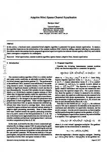
FIGURE 5-10: REAL COMPONENT OF FIRST PATH OF THE FADING CHANNEL, DOPPLER = 1 HZ. ..................................................................................................................... 104 FIGURE 5-11: DOUBLE ESTIMATION MMSE-DFE STRUCTURE. ...................................... 105 FIGURE 5-12: MMSE-DFE PERFORMANCE FOR UNKNOWN CHANNEL, DOUBLE ESTIMATION VS LINEAR INTERPOLATION, DECISION DIRECTED MODE, SYMBOL SPACED, 64QAM, 72 FRAME INTERLEAVER SIZE, =45, =5, DOPPLER=1 HZ, DELAY SPREAD=5 SYMBOLS. ............................................................................... 105 FIGURE 5-13: ITERATIVE LS CHANNEL ESTIMATION FOR FRACTIONAL SPACED INPUT. ............................................................................................................................. 106 FIGURE 5-14: MMSE-DFE PERFORMANCE FOR UNKNOWN CHANNEL, ITERATIVE LS CHANNEL ESTIMATION VS PERFECT, DECISION DIRECTED MODE, FRACTIONAL SPACED, 64QAM, 72 FRAME INTERLEAVER SIZE, =40*4, =8*4, DOPPLER = 1 HZ, DELAY SPREAD = 5 SYMBOLS. .............................................................................. 107 FIGURE 5-15: ITERATIVE MMSE-DFE EQUALIZER STRUCTURE..................................... 108 FIGURE 5-16: ITERATIVE MMSE-DFE PERFORMANCE WITH ITERATION, SYMBOL SPACED, 64QAM, 72 FRAME INTERLEAVER SIZE, =45, =5, DOPPLER = 1 HZ, DELAY SPREAD = 5 SYMBOLS. .............................................................................. 109
xiv
FIGURE 5-17: ITERATIVE MMSE-DFE PERFORMANCE, 3 ITERATIONS, ALL DATA RATES, 72 FRAME INTERLEAVER SIZE, =56 FOR ZEROS ITERATION AND 45 FOR THE OTHERS, =5, DOPPLER = 1 HZ, DELAY SPREAD = 5 SYMBOLS............................ 109 FIGURE 5-18: ITERATIVE MMSE-DFE PERFORMANCE, 1 ITERATION, FRACTIONAL SPACED VS SYMBOLS SPACED, 64QAM, 72 FRAME INTERLEAVER SIZE, =40*4 FOR FRACTIONAL SPACED AND FOR SYMBOL SPACED, =8*4 FOR FRACTIONAL SPACED AND 5 FOR SYMBOL SPACED, DOPPLER = 1 HZ, DELAY SPREAD = 5 SYMBOLS. .......................................................................................... 111 FIGURE 6-1: LINEAR FREQUENCY DOMAIN EQUALIZER STRUCTURE FOR SINGLE CARRIER ............................................................................................................... 114 FIGURE 6-2: LINEAR FD PERFORMANCE, REAL WAVEFORM, QPSK & 8PSK, 72 FRAME INTERLEAVER SIZE, DOPPLER = 1 HZ, DELAY SPREAD = 5 SYMBOLS. .................. 116 FIGURE 6-3: LINEAR FD PERFORMANCE, SAME SIGNS TRAINING, QPSK & 8PSK, 72 FRAME INTERLEAVER SIZE, DOPPLER = 1 HZ, DELAY SPREAD = 5 SYMBOLS. ...... 116 FIGURE 6-4: LINEAR FD PERFORMANCE, SAME SIGNS TRAINING, QPSK & 8PSK & 16QAM, 72 FRAME INTERLEAVER SIZE, DOPPLER = 0.5HZ, DELAY SPREAD = 5 SYMBOLS. ............................................................................................................. 117 FIGURE 6-5: ADAPTIVE LINEAR FREQUENCY DOMAIN EQUALIZER FOR SINGLE CARRIER ............................................................................................................... 118 FIGURE 6-6: ADAPTIVE LINEAR FD PERFORMANCE, REFERENCE MODE, QPSK & 8PSK, 72 FRAME INTERLEAVER SIZE, DOPPLER = 1 HZ, DELAY SPREAD = 5 SYMBOLS. ...... 119 FIGURE 6-7: ADAPTIVE LINEAR FD PERFORMANCE, REFERENCE MODE, SAME SIGNS TRAINING, QPSK & 8PSK, 72 FRAME INTERLEAVER SIZE, DOPPLER = 1 HZ, DELAY SPREAD = 5 SYMBOLS. .......................................................................................... 120 FIGURE 6-8: ADAPTIVE LINEAR FD PERFORMANCE, REFERENCE MODE, SAME SIGNS TRAINING, QPSK & 8PSK & 16QAM, 72 FRAME INTERLEAVER SIZE, DOPPLER = 0.5HZ, DELAY SPREAD = 5 SYMBOLS. ................................................................... 120 FIGURE 6-9: ADAPTIVE LINEAR FD PERFORMANCE, DECISION DIRECTED MODE, SAME SIGNS TRAINING, QPSK & 8PSK & 16QAM, 72 FRAME INTERLEAVER SIZE, DOPPLER = 0.5HZ, DELAY SPREAD = 5 SYMBOLS. ................................................................. 121 FIGURE 6-10: ITERATIVE FREQUENCY DOMAIN DECISION FEEDBACK FOR SINGLE CARRIER ............................................................................................................... 122 FIGURE 6-11: ITERATIVE FD-DFE PERFORMANCE, REFERENCE MODE, QPSK & 8PSK, 72 FRAME INTERLEAVER SIZE, DOPPLER = 1 HZ, DELAY SPREAD = 5 SYMBOLS. ...... 123 FIGURE 6-12: ITERATIVE FD-DFE PERFORMANCE, REFERENCE MODE, SAME SIGNS, ALL DATA RATES, 72 FRAME INTERLEAVER SIZE, DOPPLER = 1 HZ, DELAY SPREAD = 5 SYMBOLS. ............................................................................................................. 124 FIGURE 6-13: ITERATIVE FD-DFE PERFORMANCE, REFERENCE MODE, SAME SIGNS, ALL DATA RATES, 72 FRAME INTERLEAVER SIZE, DOPPLER = 0.5HZ, DELAY SPREAD = 5 SYMBOLS. ............................................................................................................. 124 FIGURE 6-14: ITERATIVE FD-DFE PERFORMANCE, DECISION DIRECTED MODE, SAME SIGNS, QPSK, 72 FRAME INTERLEAVER SIZE, DOPPLER = 0.5HZ, DELAY SPREAD = 5 SYMBOLS. ............................................................................................................. 125 FIGURE 6-15: ITERATIVE FD-DFE THROUGH DECODER FOR SINGLE CARRIER ............. 126 FIGURE 6-16: ITERATIVE FD-DFE THROUGH DECODER, REAL WAVEFORM, QPSK & 8PSK, 72 FRAME INTERLEAVER SIZE, DOPPLER = 1 HZ, DELAY SPREAD = 5 SYMBOLS. .. 126 FIGURE 6-17: ITERATIVE FD-DFE THROUGH DECODER PERFORMANCE, QPSK & 8PSK, 72 FRAME INTERLEAVER SIZE, DOPPLER = 0.5HZ, DELAY SPREAD = 5 SYMBOLS. .... 127
xv
FIGURE 6-18: ITERATIVE FD-DFE THROUGH DECODER PERFORMANCE, SAME SIGNS, ALL DATA RATES, 72 FRAME INTERLEAVER SIZE, DOPPLER = 0.5HZ, DELAY SPREAD = 5 SYMBOLS. .......................................................................................... 127
xvi
List of Tables TABLE 1-1: PARAMETERS USED FOR DIFFERENT DATA RATES IN MIL-STD-188-110B AND STANAG 4285. IS THE CODE RATE, IS THE NUMBER OF BITS PER CHANNEL SYMBOL, AND IS THE BANDWIDTH EFFICIENCY OF THE FRAME PATTERN [9]. .. 9 TABLE 1-2: PARAMETERS USED FOR DIFFERENT DATA RATES IN THE HIGH-RATE WAVEFORMS OF STANAG 4539 AND MIL-STD-110B [9]. ...........................................10 TABLE 1-3: MODULATION USED TO OBTAIN EACH DATA RATE ....................................16 TABLE 2-1: DOPPLER SPREAD AND DELAY SPREAD FOR THE TEST CHANNEL RECOMMENDED BY ITU-R (ITU-R F.520 [16], ITU-R F.1487 [17]) ................................41 TABLE 2-2: HIGH DATA RATE PERFORMANCE REQUIREMENTS .....................................45 TABLE 5-1: HIGH DATA RATE MODE PERFORMANCE COMPARISON BETWEEN MMSEDFE VS STANDARD REQUIREMENTS FOR 1.0E-5 BER. ........................................... 110 TABLE 7-1: COMPARISON BETWEEN DIFFERENT INTRODUCED HF EQUALIZERS WITH RESPECT TO AVERAGE SNR (DB) FOR BER NOT TO EXCEED 1.0E-5. EQUALIZER (A): ITERATIVE BI-DIRECTIONAL KALMAN-DFE. EQUALIZER (B): ITERATIVE MMSE-DFE WITH ITERATIVE DOUBLE CHANNEL ESTIMATION. EQUALIZER (C): ITERATIVE FRACTIONAL MMSE-DFE WITH ITERATIVE LS CHANNEL ESTIMATION. EQUALIZER (D): LINEAR FD. ..................................................................................................... 131 TABLE 7-2: TIME RESPONSE FOR DIFFERENT EQUALIZERS FOR ONE ITERATION FOR THE WORST CASE FOR CONSTELLATION SIZE (64 QAM) AND INTERLEAVER SIZE (72 FRAMES ~ 8.5 SEC) USING MATLAB PROFILER ON A 2.1 GHZ PROCESSOR. EQUALIZER (A): ITERATIVE BI-DIRECTIONAL KALMAN-DFE. EQUALIZER (B): ITERATIVE MMSE-DFE WITH ITERATIVE DOUBLE CHANNEL ESTIMATION. EQUALIZER (C): ITERATIVE FRACTIONAL MMSE-DFE WITH ITERATIVE LS CHANNEL ESTIMATION. EQUALIZER (D): LINEAR FD. .......................................... 131
xvii
Notations and Symbols All signals in time domain are written as lowercase italic letters for scalar, and lowercase bold letters for vectors. Signals in frequency domain are written in uppercase italic for scalar, and uppercase bold for vectors. All parameters are written in uppercase (non italic, non bold). All functions are written as bold italic. The parenthesis [] are used for discrete indexing, () for continuous indexing, and {} for statistical operations. List of Symbols Equalizer forward filter coefficient number at time Vector of Equalizer forward filter coefficients at time Vector of Frequency domain Equalizer forward filter coefficients Mixer carriers amplitudes Equalizer backward filter coefficient number at time Vector of Equalizer backward filter coefficients at time Vector contains Frequency domain of Equalizer backward filter coefficients Coded bit number m at transmitter side Coded bit number m at the receiver side Coded bit returned back from decoder Data bit number Data bit estimated Peak distortion value out of equalizer
xviii
Error signal at time index Error signal in frequency domain Expectation Bit energy Energy of tap of channel Symbol energy Least square error function Continuous frequency index Coherence bandwidth Carrier frequency Sampling frequency Channel tap gain generating filter Continuous Fourier transform of Channel tap gain generating filter g
First generating polynomial output of the convolutional encoder
g
Second generating polynomial output of the convolutional encoder Gradient vector used in LMS algorithm at time Generating polynomial function of the convolutional encoder Channel impulse response for path with delay at time Vector of channel paths at time Channel frequency response vector at time Channel equivalent impulse response including transmitter and receiver filters Discrete channel delays index Identity matrix Imaginary component of complex number MMSE cost function Discrete frequency index Index for current bit in a coded symbol Index for any bit except current bit in a coded symbol Modulation index multiplied by the coding rate xix
Kalman gain vector Equalizer taps index Log Likelihood Ratio Index of coded bits after interleaver Index of coded bits before interleaver Channel impulse response length Discrete time index Index for symbols before interleaver Discrete samples of complex baseband Gaussian process Discrete samples of the in-phase component of complex Gaussian process Discrete samples of the quadrature-phase of a complex Gaussian process Low pass continuous in-phase component of Gaussian process Low pass continuous quadrature-phase component of Gaussian process Pass band white Gaussian noise Total number of equalizer taps Number of equalizer forward taps Number of equalizer backward taps Noise power spectral density Number of training symbols Pass band noise power spectral density Number of precursor taps in equalizer filter Number of postcursor taps in equalizer filter Data bits index Average power of transmitted symbols Probability density function Discrete probability function Inverse of the correlation matrix in Kalman algorithm
xx
Equivalent filter for channel and equalizer Modulation index Discrete time received signal Vector of received signal samples Discrete Fourier transform of the received signal Vector of frequency domain samples of the received signal Spaced frequency correlation function of the channel spaced-time correlation function of the channel Receiver filter Coding rate column in the correlation matrix in MMSE Size of the alphabet Doppler power spectral density Multipath intensity profile Doppler spectrum of a tap Continuous time index Training symbols Vector of training symbols Transmitter filter Sampling frequency Coherence time Channel sampling rate Symbol time Correlation function used in Kalman algorithm Signal variance Noise bandwidth Signal bandwidth Transmitted signal samples Vector of transmitted signal samples Discrete Fourier transform of transmitted signal xxi
Vector of transmitted signal in frequency domain Estimated transmitted signal (soft equalizer output) Estimated transmitted signal returned back from the decoder Hard decisions of estimated transmitted signal Average of the transmitted signal Cross-correlation vector used in Kalman algorithm Z domain samples index Iteration factor in the iterative frequency domain DFE equalizer Square root raised cosine roll-off factor Small positive constant used in Kalman algorithm Small positive number used in LMS algorithm AWGN discrete noise samples AWGN continuous noise samples Factor to simplify the MMSE equation when using a priori input Correlation matrix used in MMSE Correlation matrix for the forward filter in a DFE MMSE equalizer Correlation matrix for the backward filter in a DFE MMSE equalizer Small positive number used in frequency domain LMS equalizer Matrix contains the training symbols Doppler frequency Doppler spread Mean value of the Doppler spectrum Vector contains received samples and hard decisions of the previous symbols Noise variance Channel path delay (continuous time) Delay spread The channel output during training sequence Vector of equalizer forward and backward filter coefficients
xxii
Abbreviations 2G
Second Generation
3G
Third Generation
AGC
Automatic Gain Control
ALE
Automatic Link Establishment
AM
Amplitude modulation
AWGN
Additive White Gaussian Noise
BCJR
Bahl, Cocke, Jelinek and Raviv algorithm for maximum a posteriori decoding
BER
Bit Error Rate
BLOS
beyond Line of Sight
BW
Band Width
CIR
Channel Impulse Response
CMA
Constant Modulus Algorithm
DFE
Decision Feedback
DO
Design Objective
ECC
Error-correcting code
FBF
Feedback Filter
FD
Frequency Domain
FFF
Feed Forward Filter
FFT
Fast Fourier Transform
FIR
Finite Impulse Response
FRLS
Fast Recursive Least Squares
FSE
Fractionally Spaced Equalizer xxiii
FSK
Frequency shift keying
HF
High Frequency
IFFT
Inverse Fast Fourier Transform
IIR
Infinite Impulse Response
ISI
Inter Symbol Interference
ITU
International Telecommunications Union
LLR
Log Likelihood Ratio
LMS
Least Mean Square
LOS
Line of Sight
LS
Least Square
LSB
Lower Sideband or Least Significant bit
MAP
Maximum A posteriori Probability
MIL-STD
Military Standard (series published by US DoD)
MLSE
Maximum Likelihood Sequence Estimator
MMSE
Minimum Mean Square Error
MSB
Most Significant bit
OFDM
Orthogonal Frequency Division Multiplexing
OSI
Open Systems Interconnection
PAR
Peak to Average power Ratio
PSK
Phase Shift Keying
QAM
Quadrature Amplitude Modulation
QPSK
Quadrature Phase Shift Keying
RLS
Recursive Least squares
RX
Receiver
SC-FDE
Single Carrier Frequency Domain Equalization
SISO
Soft Input Soft Output
SNR
signal to Noise Ratio
SRRC
Square Root Raised Cosine filter
SSB
Single Sideband
STANAG
Standardization Agreement (series published by NATO)
TX
Transmitter xxiv
UHF
Ultra High Frequency
US DoD
United States Department of Defense
USB
Upper Sideband
VHF
Very High Frequency range
VLSI
Very Large Scale Integration
VoIP
Voice over Internet Protocol
WMF
Whitened Matched Filter
WSSUS
Wide Sense Stationary Uncorrelated Scattering
XOR
Exclusive OR
ZF
Zero Forcing
xxv
Chapter 1
Introduction to HF Communications 1
Introduction to HF co mmunications
1.1 Principles of HF radio communications 1.1.1 Radio frequency spectrum In the radio frequency spectrum (Figure 1-1), the usable frequency range for radio waves extends from about 20 kHz (just above sound waves) to above 30000 MHz (A wavelength ranges from 15 kilometers long at 20 kHz to 1 centimeter at 30000 MHz). The HF band is defined as the frequency range of 3 to 30 MHz. In practice, most HF radios use the spectrum from 1.6 to 30 MHz. Most long-haul communications in this band take place between 4 and 18 MHz. Higher frequencies (18 to 30 MHz) may also be available from time to time, depending on ionospheric conditions and the time of day. In the early days of radio, HF frequencies were called short wave because their wavelengths (10 to 100 meters) were shorter than those of commercial broadcast stations. The term is still applied to long-distance radio communications.
1
Figure 1-1: Radio frequency spectrum [1]
1.1.2 Modulation Today’s common methods for radio communications include amplitude modulation (AM), where the information is contained in amplitude variations. AM is a relatively inefficient form of modulation, since the carrier must be continually generated. The majority of the power in an AM signal is consumed by the carrier that carries no information, with the rest going to the information carrying sidebands. In a more efficient technique, single sideband (SSB), the carrier and one of the sidebands are suppressed. Only the remaining sideband, upper (USB) or lower (LSB), is transmitted. An SSB signal needs only half the bandwidth of an AM signal and is produced only when a modulating signal is present. Thus, SSB systems are more efficient both in the use of the spectrum, which must accommodate many users, and of transmitter power. All the transmitted power goes into the information-carrying sideband.
2
1.1.3 Radio wave propagation Propagation describes how radio signals radiate outward from a transmitting source. The action is simple to imagine for radio waves that travel in a straight line. The true path radio waves take, however, is often more complex. There are two basic modes of propagation: ground waves and sky waves. As their names imply, ground waves travel along the surface of the earth, while sky waves “bounce” back to earth. Figure 1-2 shows the different propagation paths for HF radio waves. Ground waves consist of three components: surface waves, direct waves, and ground-reflected waves. Surface waves travel along the surface of the earth, reaching beyond the horizon. Eventually, surface wave energy is absorbed by the earth. The effective range of surface waves is largely determined by the frequency and conductivity of the surface over which the waves travel. Absorption increases with frequency. Direct waves travel in a straight line, becoming weaker as distance increases. They may be bent, or refracted, by the atmosphere, which extends their useful range slightly beyond the horizon. Transmitting and receiving antennas must be able to “see” each other for communications to take place, so antenna height is critical in determining range. Because of this, direct waves are sometimes known as line-of-sight (LOS) waves. Ground-reflected waves are the portion of the propagated wave that is reflected from the surface of the earth between the transmitter and receiver. Sky waves make beyond line-of-sight (BLOS) communications possible. At certain frequencies, radio waves are refracted (or bent), returning to earth hundreds or thousands of miles away. Depending on frequency, time of day, and atmospheric conditions, a signal can bounce several times before reaching a receiver. Using sky waves can be tricky, since the ionosphere is constantly changing.
3
Figure 1-2: Propagation paths for HF radio waves [1]
1.2 Importance of HF communications From the advent of radio communications in the late 19th century until the 1960’s, radio communications using frequencies in and below the HF band was the only alternative for long-range communication. And even after the advent of other means of long-range communication, HF radio still has several important advantages over other communications media. Government and private organizations involved in emergency and remote communications are continually searching for the most flexible, reliable and cost effective solutions for their communications needs. HF communication provides all of these proprieties which make it a vital and irreplaceable wireless communications tool for these organizations. We can summarize the advantages of HF communication over other communications media in the following points,
4
Long range communications capability Whilst VHF and UHF radio is also commonly used for short-range line-of sight (LOS) communications, HF is capable of communicating over distances of 3000 km or more (often inter-continental). Minimal infrastructure requirements Unlike conventional, VoIP, cellular and satellite telephony, which all rely upon land-based infrastructure or satellite, an HF radio network requires minimal infrastructure. As such it is often the only reliable means of communication when disaster strikes. Full mobility HF radio is simple and quick to deploy and provides communications capability for users no matter where they are. Fixed base stations can be used to communicate with other bases or to provide command and control for mobile (vehicle-mounted) and portable (man-pack) users in the field. Low cost of ownership Compared with satellite telephony, the most common alternative technology for communications of last resort, HF radio is the economical choice. Once the initial investment in equipment is made, there are no call costs or ongoing monthly line or equipment rentals. Also, HF radio equipment is built tough to withstand the extreme conditions, which proves to be very cost-effective. Security and reliability Satellite transponders are vulnerable to jamming from the earth as well as small countries, like Egypt, cannot always be guaranteed capacity on a satellite owned by another country. Which make HF communications the last resort in emergencies and when disaster strikes.
5
New standards for HF communications The introduction of several new standards for HF communications in 1990’s, as well as the rapid development of digital signal processing during the last decade make HF communication more easier to operate and also improve the performance in terms of availability and data rates.
1.3 Standards in military HF communications Standards for military communications are being developed by NATO (North Atlantic Treaty Organization), and by US DoD (United States Department of Defense). The STANAG (Standardization Agreement) series is published by NATO, and the MIL-STD (Military Standard) series is published by US DoD. STANAGs often have MIL-STD counterparts, with only subtle differences.
1.3.1 HF house NATO has developed a reference framework to describe the relationship between the different standards for HF communications. This framework is called “the HF house”, and is shown in Figure 1-3 The HF house relates to the lower three layers of the OSI (Open Systems Interconnection) Framework: The physical layer (layer 1), the data link layer (layer 2), and the network layer (layer 3). At the physical layer there are different waveform standards, and at layers 2 and 3 there are standards for automatic repeat request, networking, link setup, and link maintenance. Interfaces to higher layers of the OSI framework are also included in the HF house.
6
Figure 1-3: HF house (included in most of the recent NATO STANAGs on HF communications)
In particular, 2G systems like STANAG 5066 [2] were developed for maritime communications, whereas 3G systems like STANAG 4538 [3] were designed for ground tactical communications. It is also possible to combine 2G and 3G systems.
1.3.2 Waveform standards Most frequency assignments in the military HF bands have a bandwidth of 3 kHz. This is for historical reasons; 3 kHz was the bandwidth needed for analog voice using SSB (single sideband) modulation. Also, HF modems are often connected to the audio (voice) interface of an HF radio, which has a bandwidth of approximately 2.7 kHz. This bandwidth limitation puts constraints on the maximum available data rate for HF modems. In HF terminology, the word “waveform” is used to describe the entire baseband signal processing at the physical layer in the transmitter, i.e., the conversion from data bits to the signal delivered to the audio interface of the radio. This encompasses e.g. pulse shaping, signal constellations, frame
7
structure, and error correcting coding. HF radios use SSB modulation to convert the input audio signal (the “waveform”) to the transmitted RF signal. When designing HF waveforms, three fundamentally different approaches are used: Frequency shift keying (FSK), parallel-tone waveforms, and serial-tone waveforms. FSK is inefficient in terms of power as well as bandwidth, and is currently used mainly in the link setup waveforms in 2G ALE. Parallel-tone waveforms (OFDM) are described in optional appendices to MIL-STD-188110B [4]: Appendix A describes a 16-tone waveform, and Appendix B describes a 39- tone waveform. Most other waveforms included in the HF house are serial-tone waveforms. Nieto in [5] has compared the characteristics and performance of serial-tone and parallel-tone waveforms. His conclusion is that the basic performance of the two approaches is similar, but the ECC (error-correcting code) used in the serial-tone waveform standards performs better than the ECC used in the parallel-tone waveform standards. For this reason, serial-tone waveforms have gained popularity. However, serial-tone receiver requires adaptive equalization as an essential component, which is more complex than the receiver used in parallel-tone. In this work, we concentrate on serial-tone waveforms, as these are the most commonly used waveforms for military HF communications. In the following sections, different serial-tone waveforms are described.
1.3.2.1 Robust low rate HF waveforms A very robust low-rate waveform with an information data rate of 75 bps is described in STANAG 4415 [6]. The same waveform is also defined for 75 bps in MIL-STD-188-110B, but the performance requirements are much stricter in STANAG 4415 a modem which is compliant to STANAG 4415 is a good choice under severe conditions at high latitudes, if one needs high probability of being able to communicate and can cope with the low data rate. 8
1.3.2.2 Medium rate serial tone HF waveforms Two different medium-rate waveforms can be found within the HF house; one is described in MIL-STD-188-110B (this waveform was also included in the older version of the standard, MIL-STD-188-110A), and the other is described in STANAG 4285 [7]. The newer NATO waveform standard STANAG 4539 [8], which includes all data rates in the range 75-12800 bps, points to MILSTD-188-110B for data rates of 2400 bps and below. Table 1-1 summarizes the code rate, signal constellation size, and frame pattern used for each data rate in MIL-STD-188-110B and STANAG 4285. Both standards also define one data rate above 2400 bps, which does not use any ECC. These waveforms suffer from very high bit error rates because they are un-coded, and they are therefore seldom used in practice. The 75 bps waveform in MIL-STD-188-110B is similar to the robust waveform.
Table 1-1: Parameters used for different data rates in MIL-STD-188-110B and STANAG 4285. and
is the code rate,
is the number of bits per channel symbol,
is the bandwidth efficiency of the frame pattern [9].
9
1.3.2.3 High rate serial tone HF waveforms High rate serial tone HF waveforms are described in Annex B of STANAG 4539 and in Appendix C of MIL-STD-188-110B. These two standards describe identical high-rate waveforms; the only difference is that the performance requirements of STANAG 4539 are stricter. Table 1-2 summarizes the parameters for each data rate in the high-rate waveforms (compare to Table 1-1 for the medium-rate waveforms). 12800 bps can be achieved if the ECC is omitted, but for all the other data rates (32009600 bps), the only parameter that is changed is the signal constellation.
Table 1-2: Parameters used for different data rates in the high-rate waveforms of STANAG 4539 and MIL-STD-110B [9].
1.4 Current HF standard (Transmitter model) Figure 1-4 shows the structure of the transmitter for High rate serial tone HF (Annex B of STANAG 4539 and Appendix C of MIL-STD-188-110B). In the following, we go through each block.
11
Block Processing
d [o ]
Convolution Encoding
Blocking
ct [m]
Interleaving
Frame Processing
ct [m]
Scrambling
Modulation
Initial Preamble
MiniProbes
Modulation (8 PSK)
Framing
Reinserted Preamble
Upsample
x[n]
SRRC Filter
Figure 1-4: HF Transmitter structure
1.4.1 Blocking The blocking is responsible of dividing the raw bits to blocks of size dependent on the Rate and the Inter-leaver length (shown in table C-XIV in [4]). Each code block shall be interleaved within a single inter-leaver block of the same size. The boundaries of these blocks shall be aligned such that the beginning of the first data frame following each reinserted preamble shall coincide with an inter-leaver boundary.
1.4.2 Convolutional encoding The full-tail-biting and puncturing techniques shall be used with a rate 1/2 convolutional code to produce a rate 3/4 block code that is the same length as the inter-leaver. A constraint length 7, rate 1/2 convolutional code shall be used prior to puncturing. Figure 1-5 is a pictorial representation of the encoder. The two summing nodes in the figure represent modulo 2 additions. For each bit input to
11
the encoder, two bits are taken from the encoder, with the upper output bit,
taken first.
To implement the full-tail-biting, the encoder shall be preloaded by shifting in the first six input data bits without taking any output bits. These six input bits shall be temporarily saved so that they can be used to flush the encoder. The first two coded output bits shall be taken after the seventh bit has been shifted in, and shall be defined to be the first two bits of the resulting block code. After the last input data bit has been encoded, the first six (saved) data bits shall be encoded. The encoded bits shall be the final bits of the resulting (unpunctured) block code. Prior to puncturing, the resulting block code will have exactly twice as many bits as the input information bits. Puncturing of the rate 1/2 code to the required rate 3/4 shall be done prior to sending bits to the interleaver. In order to obtain a rate 3/4 code from the rate 1/2 code used, the output of the encoder must be punctured by not transmitting 1 bit out of every 3. Puncturing shall be performed by using a puncturing mask of
, applied to the
bits output from the encoder. In this notation a 1 indicates that the bit is retained and a 0 indicates that the bit is not transmitted. For an encoder generated sequence of, g
g
g
g
g
g
g
g
The transmitted sequence shall be, g
g
1.4.3 Interleaving Convolutional codes perform well when bit errors are uncorrelated, but are less effective than block codes in bursty error patterns. On HF channels, such bursty error patterns are caused by fading and impulsive noise and interference, and Convolutional codes would be a bad choice unless further precautions were taken. 12
G1(D) +
INPUT
D6
D 5 D4
D 3 D2 D
1
OUTPUT
+
G2 (D) Constraint length = 7 Generator Polynomials:
G1 (D) D6 D4 D3 D 1 G2 (D) D6 D5 D4 D3 1
Figure 1-5: Tail biting Convolutional encoder
For this reason, an interleaver is used. The block interleaver used is designed to separate neighboring bits in the punctured block code as far as possible over the span of the interleaver with the largest separations resulting for the bits that were originally closest to each other. Generally, a longer interleaver gives better performance, and the interleaver should at least be longer than the maximum duration of a fade or noise burst. But, a longer interleaver also gives a larger delay (latency), which is undesirable for some applications. The interleaver shall consist of a single dimension array, numbered from its
to
. The array size shall depend on both the data rate and 13
interleaver length (as shown in table C-XV in [4]). Defining the first punctured block code bit to be Load Location = (
, then the load location for
is given by:
* Interleaver Increment Value) Modulo (Interleaver Size in Bits)
where, Interleaver Increment Value is specified in (table C-XVI in [4]). These increment values have been chosen to ensure that the combined cycles of puncturing and assignment of bit positions in each symbol for the specific constellation being used is the same as if there had been no interleaving. This is important, because each symbol of a constellation contains "strong" and "weak" bit positions, except for the lowest data rate. Bit position refers to the location of the bit, ranging from MSB to LSB, in the symbol mapping. A strong bit position is one that has a large average distance between all the constellation points where the bit is a 0 and the closest point where it is a 1. Typically, the MSB is a strong bit and the LSB a weak bit. An interleaving strategy that did not evenly distribute these bits in the way they occur without interleaving could degrade performance. The fetching sequence for all data rates and interleaver lengths shall start with location 0 of the interleaver array and increment the fetch location by 1. This is a simple linear fetch from beginning to end of the interleaver array.
1.4.4 Scrambling Data symbols for the 8PSK symbol constellation (3200 bps, 4800 bps) shall be scrambled by "modulo 8 additions" with a scrambling sequence. The data symbols for the 16QAM, 32QAM, and 64QAM constellations shall be scrambled by using an "exclusive or (XOR) operation". In all cases, the scrambling sequence generator polynomial shall be
and the
generator shall be initialized to 1 at the start of each data frame. A block diagram of the scrambling sequence generator is shown in Figure 1-6.
14
For 8PSK symbols (3200 bps and 4800 bps), the scrambling shall be carried out taking the modulo-8 sum of the numerical value of the binary triplet consisting of the last (rightmost) three bits in the shift register, and the symbol number (transcoded value). For 16QAM symbols, scrambling shall be carried out by XORing the 4 bit number consisting of the last (rightmost) four bits in the shift register with the symbol number.
0
D8
0
D7
0
D6
0
D5
0
D4
0
D3
0
D2
0
D
1
+ Scrambling Symbols
Figure 1-6: Scrambler
For 32QAM symbols, scrambling shall be carried out by XORing the 5 bit number formed by the last (rightmost) five bits in the shift register with the symbol number. For 64QAM symbols, scrambling shall be carried out by XORing the 6 bit number formed by the last (rightmost) six bits in the shift register with the symbol number. After each data symbol is scrambled, the generator shall be iterated (shifted) the required number of times to produce all new bits for use in scrambling the next symbol (i.e., 3 iterations for 8PSK, 4 iterations for 16QAM, 5 iterations for 32QAM and 6 iterations for 64QAM). Since the generator is iterated after the bits are use, the first data symbol of every data frame shall, therefore, be scrambled by the appropriate number of bits from the initialization value of “00000001”.
15
The length of the scrambling sequence is 511 bits. For a 256 symbol data block with 6 bits per symbol, this means that the scrambling sequence will be repeated just slightly more than 3 times, although in terms of symbols, there will be no repetition.
1.4.5 Modulation 1.4.5.1 Data symbols For data symbols, the modulation used shall depend upon the data rate. The Table 1-3 specifies the modulation that shall be used with each data rate.
Table 1-3: Modulation used to obtain each data rate
The 3200 bps quadrature phase-shift keying (QPSK) constellation is scrambled to appear, on-air, as an 8PSK constellation. Both the 16QAM and 32QAM constellations use multiple PSK rings to maintain good peak-to-average ratios, and the 64QAM constellation is a variation of the standard square QAM constellation, which has been modified to improve the peak-to-average ratio. 1.4.5.1.1 PSK data symbols For the PSK constellations, a distinction is made between the data bits and the symbol number for the purposes of scrambling the QPSK modulation to appear 16
as 8PSK, on-air. Scrambling is applied as a modulo-8 addition of a scrambling sequence to the 8PSK symbol number. Transcoding is an operation which links a symbol to be transmitted to a group of data bits. Transcoding for both 3200 and 4800 bps user data rate are specified in table C-III and table C-IV in [4] respectively. PSK symbol mapping is shown in Figure 1-7.
Figure 1-7: PSK symbol mapping
1.4.5.1.2 QAM data symbols For the QAM constellations, no distinction is made between the number formed directly from the data bits and the symbol number. Each set of 4 bits (16QAM), 5 bits (32QAM) or 6 bits (64QAM) is mapped directly to a QAM symbol. The mapping of bits to symbols for the QAM constellations has been selected to minimize the number of bit errors incurred when errors involve adjacent signaling points in the constellation.
17
The constellation points which shall be used for 16QAM are shown in the Figure 1-8 and specified in terms of their In-phase and Quadrature components in table C-V in [4]. As can be seen in the Figure 1-8, the 16 QAM constellation is comprised of two PSK rings: 4 PSK inner and 12 PSK outer. The constellation points which shall be used for 32QAM are shown in the Figure 1-9 and specified in terms of their In-phase and Quadrature components in table C-VI in [4]. This constellation contains an outer ring of 16 symbols and an inner square of 16 symbols. The constellation points which shall be used for the 64QAM modulation are shown in Figure 1-10 and specified in terms of their In-phase and Quadrature components in table C-VII in [4]. This constellation is a variation on the standard 8 x 8 square constellation, which achieves better peak to average without sacrificing the very good pseudo-Gray code properties of the square constellation.
Figure 1-8: 16QAM Signaling Constellation.
18
Figure 1-9: 32QAM signaling constellation.
Figure 1-10: 64QAM signaling constellation.
19
1.4.5.2 Known symbols For all known symbols, the modulation used shall be PSK, with the symbol mapping shown in table C-I in [4] and Figure 1-7. No scrambling shall be applied to the known symbols.
1.4.6 Framing construction The frame structure that shall be used for the waveforms specified in this protocol is shown in Figure 1-11. An initial 287 symbol preamble is followed by 72 frames of alternating data and known symbols. Each data frame shall consist of a data block consisting of 256 data symbols, followed by a miniprobe consisting of 31 symbols of known data. After 72 data frames, a 72 symbol subset of the initial preamble is reinserted to facilitate late acquisition, Doppler shift removal, and sync adjustment. It should be noted that the total length of known data in this segment is actually 103 symbols: the 72 reinserted preamble symbols plus the preceding 31 symbol mini-probe segment which follows the last 256 symbol data block.
Figure 1-11: Frame structure for all waveforms.
21
1.4.6.1 Synchronization preamble The synchronization preamble is used for rapid initial synchronization. The synchronization preamble shall consist of two parts. The first part shall consist of at least N blocks of 184 8-PSK symbols to be used exclusively for radio and modem AGC. These 184 symbols shall be formed by taking the complex conjugate of the first 184 symbols of the sequence specified below for the second section. The second section shall consist of 287 symbols. The first 184 symbols are intended exclusively for synchronization and Doppler offset removal purposes while the final 103 symbols, which are common with the reinserted preamble, also carry information regarding the data rate and interleaver settings. Expressed as a sequence of 8PSK symbols, using the symbol numbers given in the 8PSK table the synchronization preamble shall be as shown in table C-VIII in [4].
1.4.6.2 Reinserted preamble The reinserted preamble shall be identical to the final 72 symbols of the synchronization preamble. In fact, the final 103 symbols are common between the synchronization preamble and the contiguous block consisting of the reinserted preamble and the mini-probe which immediately precedes it. The 103 symbols of known data (including the 31 mini-probe symbols of the preceding data frame) are shown in table C-XI in [4]. The first 31 of these symbols are the immediately preceding mini-probe, which follows the last of the 72 data blocks.
1.4.6.3 Mini-probes Mini-probes 31 symbols in length shall be inserted following every 256 symbol data block and at the end of each preamble (where they are considered to be part of the preamble). Using the 8PSK symbol mapping, each mini-probe shall
21
be based on the repeated Frank-Heimiller sequence. The sequence that shall be used specified in terms of the 8PSK symbol numbers is given by, 0, 0, 0, 0, 0, 2, 4, 6, 0, 4, 0, 4, 0, 6, 4, 2, 0, 0, 0, 0, 0, 2, 4, 6, 0, 4, 0, 4, 0, 6, 4
This mini-probe will be designated '+'. The phase inverted version of this sequence will be designated ' - ', as the phase of each symbol has been rotated 180 degrees from the '+'. There are a total of 73 mini-probes for each set of 72 data blocks. For convenience, each mini-probe will be sequentially numbered, with mini-probe 0 being defined as the last 31 symbols of the preceding (reinserted) preamble, mini-probe number 1 following the first data block after a (reinserted) preamble. Mini-probe 72 follows the 72nd data block, and is also the first 31 symbols of the next 103 symbol reinserted preamble. Mini-probes 0 and 72 have been defined as part of the reinsertion preamble to have the signs - and + respectively. The data rate and interleaver length information encoded into the synchronization and reinserted preambles shall also be encoded into miniprobes 1 through 72. (For more details refer to section C.5.2.2 in [4]).
1.4.7 Transmitter filter The power spectral density of the modulator output signal should be constrained to be at least 20 dB below the signal level measured at 1800 Hz, when tested outside of the band from 200 Hz to 3400 Hz. The filter employed shall result in a ripple of no more than ±2 dB in the range from 800 Hz to 2800 Hz. The designed filter is a square root raised cosine filter with roll-off 0.25. The impulse response of the filter shown in Figure 1-12 is of length is symbol time (
, where
). The frequency response of the
filter is shown in Figure 1-13.
22
0.4
0.35
0.3
0.25
0.2
0.15
0.1
0.05
0
-0.05
-0.1 -6
-4
-2
the Time unitis T
0
2
4
where T = 1/2400 sec
Figure 1-12: Transmitter filter (SRRC) Impulse Response
Figure 1-13: Transmitter filter (SRRC) frequency response
23
6
1.5 Receiver structure Figure 1-14 shows the receiver basic structure. It starts with the equalization process then the reverse operations for transmitter blocks. The decoder is a Viterbi decoder supporting tail biting initialization. Some blocks are missing in that diagram like time synchronization (detection for frame start) and frequency synchronization (carrier offset cancellation and sampling clock recovery). The receiver filter (SRRC) could be removed if fractional equalizer is used.
r[n ]
Receiver Input
SRRC
De-Framming
t [n ]
Equalizer
Demodulation (Soft Decision)
Deinterleaving
Descrambling
~ d [o ] Decoder
Figure 1-14: Receiver Basic Structure
1.6 Main contributions Iterative Bi-directional Kalman DFE (fractional spaced) o Outperforms conventional Kalman DFE with (~10 dB) for both QPSK and 8PSK. o Works with all data rates, while conventional Kalman DFE can work properly with QPSK and 8PSK only.
24
o Meets standard requirements for (QPSK, 8PSK and 16QAM) with 1~2 dB margin and out of standard for 32QAM and 64QAM with loss 1~2 dB. Iterative MMSE DFE with iterative double channel estimation o Much simpler than turbo equalizer. o Meets the standard requirements with margin ~5.2 dB for 64QAM. Iterative MMSE DFE fractional spaced equalizer with iterative LS channel estimation o Complete and realistic equalizer for HF channel (tested under real poor channel). o Meets the standard requirements with ~2.5 dB for 64QAM. Frequency domain equalization for HF single carrier system o Succeeded only with QPSK with very low complexity linear equalizer. o Linear FD failed to mitigate rates greater than 8PSK, while Iterative FD DFE through decoder can work but out of standard. o Could be an optimum solution for medium data rates standards.
1.7 Outline of the thesis This thesis is a monograph, where chapters 1, 2 and 3 contain material of introductory and tutorial nature, while other chapters contain our major research contributions. In chapter 2 we give an introduction to channel effects and an overview for HF standard channel. In chapter 3 we give a survey for channel equalization. In
25
chapter 4 we tried the conventional Kalman-DFE with current HF standard and present some new ideas to enhance its performance, like bi-directional and iterative processing. In chapter 5 we apply the MMSE algorithm to HF and several new ideas are presented to enhance its performance, like iterative equalization and iterative double channel estimation. The fractional spaced MMSE is also introduced with some modifications in LS channel estimation. In chapter 6 an availability study is presented for frequency domain equalization for the HF channel, also some ideas like iterative equalization is tested. Chapter 7 contains the conclusions for the research and chapter 8 presents some suggestions for future work.
26
Chapter 2
HF Channel 2
HF Cha nnel
In this chapter we discuss the different effects of the channel on wireless transmission. The channel model for these effects is also explained. For more details on these basics, refer to [10], [11], [12] and [13]. Finally, the HF channel model is described including all parameters specified in the current standard.
2.1 Additive White Gaussian Noise (AWGN channel) Studying the AWGN is usually the starting point of understanding the basic performance relationships. The primary source of performance degradation is thermal noise generated in the receiver. AWGN is an additive noise, its power spectral density is assumed to be constant (white) over the signal bandwidth, noise samples have a Gaussian distribution with zero mean and assumed to be statistically independent.
27
2.1.1 Baseband equivalent of band pass Gaussian noise 2.1.1.1 Band pass Gaussian noise In communication system studies, it is common to utilize an additive white Gaussian noise (AWGN) model with double-sided power spectral density for the channel. If white Gaussian noise is passed through an ideal band pass filter, then the result is band pass white Gaussian noise with power spectral density
, shown in Figure 2-1. (2.1)
Wn
No/2
fc
f
fc
Figure 2-1: Band pass Gaussian noise
That is, the noise spectrum is flat over bandwidth frequency . If
in the vicinity of carrier
, then the time domain samples noise
can be
represented as a narrow band stochastic process [13] (2.2)
where
are two independent real low pass Gaussian processes.
2.1.1.2 Baseband equivalent Gaussian noise Baseband equivalence of narrowband pass signal (complex envelope) has been used extensively in analysis and design of digital communication systems, for 28
its simplicity (in both analysis and design) and efficient processing (on a lower processing speed). The general procedure to convert the baseband to equivalent band pass and vice versa is shown in Figure 2-2. To maintain the same energy of the signal in both complex baseband and pass band equivalent,
should be
and hence, the
corresponding power spectral density of the noise in the complex baseband is (or
for real and
for imaginary). Es
Re
2Es /Ac2
No/Ac2
Complex
0 Wn
X
0
2No/Ac2
Ac . cos(2f ct )
Wn
No/2
+
Im
fc
Wn
fc
f
2 c
No/A 0
X
Wn
Ac .sin(2f ct )
Figure 2-2: Convert from band pass to baseband
2.1.2 Signal to Noise ratio The relation of signal to noise in AWGN can be described by different quantities such as,
(Symbol energy to Noise power spectral density).
(Bit energy to Noise power spectral density).
SNR (Signal power to noise power ( signal and noise power respectively).
29
), where,
are the
2.1.2.1 Symbol energy to noise power spectral density (
)
The basic ratio, as noise usually added to transmitted symbols, and can be converted to other ratios as we will see in the following sections.
2.1.2.2 Bit energy to noise power spectral density (
)
The famous quantity used in performance measurements. We can convert simply from (
) to (
) using the following relation,
(2.3)
where,
, and,
2.1.2.3 Signal power to noise power (SNR) Current HF standard uses SNR in its performance measurement. However, to use SNR, we should first specify the bandwidth of noise measurement KHz for HF standard), and then the conversion from
(3
to SNR will be as
follows, (2.4)
(2.5)
(2.6)
For
(where,
is the sampling frequency)
(2.7)
For
and
(HF standard measurements),
31
(2.8)
9 9
2.2 Channel Fading In a wireless mobile communication system, a signal can travel from transmitter to receiver over multiple reflective paths; this phenomenon is referred to as multipath propagation. The effect can cause fluctuations in the received signal’s amplitude, phase, and angle of arrival, giving rise to the terminology multipath fading. Another name, scintillation, which originated in radio astronomy, is used to describe the multipath fading caused by physical changes in the propagating medium, such as variations in the density of ions in the ionospheres' layers that reflect high-frequency (HF) radio signals.
2.2.1 Channel fading effects 2.2.1.1 Delay spread (Time spreading) A multipath propagation results in receiving multiple delayed copies of the signal, the signal's propagation delay that exceeds the delay of the first signal arrival at the receiver is called the excess delay ( ). Maximum excess delay (
) is defined as the time between the first and last received components.
Figure 2-3a shows what is called a multipath intensity profile, delay . delay
versus time
represents the variation of average received power with time variation. Figure 2-3b shows the equivalent Fourier transform of
called spaced frequency correlation function
.
,
can be thought of
as the channel’s frequency transfer function. Therefore, the time-spreading manifestation can be viewed as if it were the result of a filtering process. Knowledge of
helps us to know the correlation between received signals
that are spaced in frequency
. 31
Figure 2-3: Relationship among the channel correlation functions and power spectral functions. [11]
The coherence bandwidth,
, is a statistical measure of the range of
frequencies over which the signal’s spectral components are affected by the channel in a similar manner. Note that
and
are reciprocally related
(within a multiplicative constant). As an approximation, it is possible to say that 32
(2.9)
2.2.1.2 Time variance The time-varying nature of the channel results from the relative motion between a transmitter and receiver, or by movement of objects within the channel. Figure 2-3d shows a Doppler power spectral density function of Doppler frequency shift . Knowledge of
, as a
allows us to know
how much spectral broadening is imposed on the signal as a function of the rate of change in the channel state. The width of the Doppler power spectrum is referred to as the spectral broadening or Doppler spread, denoted by
. The Doppler spread
is also
regarded as the typical fading rate of the channel. In a typical multipath environment, the received signal arrives from several reflected paths with different path distances and different angles of arrival, and the Doppler shift of each arriving path is generally different from that of another path. The effect on the received signal is seen as a Doppler spreading or spectral broadening of the transmitted signal frequency, rather than a shift. viewed in Figure 2-3d corresponds is a result of the dense-scatterer channel model and matches experimental data gathered for mobile radio channels, however, different applications yield different spectral shapes. For example
is a Gaussian shape in HF system (Watterson channel model).
The sharp upper limit on the Doppler shift produced by a vehicular antenna traveling among the stationary scatterers of the dense-scatterer model (magnitude of the frequency shift) is given by, vehicular velocity and
, where,
is the
is the wave length.
Figure 2-3c shows the function
, designated the spaced-time correlation
function; it is the corresponding inverse Fourier for
. Knowing
yields knowledge about the span of time over which two received signals have 33
a strong potential for amplitude and phase correlation. ( ) was described as the expected time duration over which the channel’s response is essentially invariant, and is called coherence time. We should note also that
and
are
reciprocally related, therefore, the approximate relationship can be as . Another definition for
as the time to traverse a distance
/2 (two
adjacent nulls) when travelling at a constant velocity ,
(2.10)
2.2.2 Degradation categories due to signal Time-spreading In a fading channel, the relationship between maximum excess delay time, and symbol time,
,
, can be viewed in terms of two different degradation
categories,
2.2.2.1 Flat fading A channel is said to exhibit frequency nonselective or flat fading if
.
In this case, all the received multipath components of a symbol arrive within the symbol time duration; hence, the components are not resolvable. Here, there is no channel-induced ISI distortion, since the signal time spreading does not result in significant overlap among neighboring received symbols. There is still performance degradation since the irresolvable phasor components can add up destructively to yield a substantial reduction in SNR. Another view in frequency domain, that flat fading degradation occurs whenever
. Hence, all of the signal’s spectral components will be
affected by the channel in a similar manner (e.g., fading or no fading). We should also note that signals which classified as exhibiting flat fading can sometimes experience frequency-selective distortion, where the null of the channel’s frequency transfer function occurs at the center of the signal band. 34
2.2.2.2 Frequency selective fading A channel is said to exhibit frequency-selective fading if
. This
condition occurs whenever the received multipath components of a symbol extend beyond the symbol’s time duration. Such multipath dispersion of the signal yields the same kind of ISI distortion caused by an electronic filter. In fact, another name for this category of fading degradation is channel-induced ISI. Also, we can say that a channel is referred to as frequency-selective if
, where the symbol rate,
to the signal bandwidth
is nominally taken to be equal
. Frequency-selective fading distortion occurs
whenever a signal’s spectral components are not all affected equally by the channel. i.e., some of the signal's width will be affected differently (outside coherence bandwidth). In order to avoid channel induced ISI distortion, the channel is required to exhibit flat fading by ensuring that if coherence bandwidth
. Hence, the channel
sets an upper limit on the transmission rate that can be
used without incorporating an equalizer in the receiver.
2.2.3 Degradation categories due to signal Time-variance The time variant nature of the channel or fading rapidity mechanism can be viewed in terms of two degradation categories,
2.2.3.1 Slow fading A channel is referred to as slow fading if the signaling rate is greater than the fading rate, (
. Or, we can say a channel is generally referred to as
introducing slow fading if
. Here, the time duration that the channel
behaves in a correlated manner is long compared to the time duration of a transmission symbol. The primary degradation in a slow-fading channel, as with flat fading, is loss in SNR.
35
2.2.3.2 Fast fading A channel is referred to as fast fading if the symbol rate, equal to the signaling rate or bandwidth (approximately equal to
(approximately
) is less than the fading rate,
); that is, fast fading is characterized by, (
Or, from the other view, fast fading occurs when channel coherence time and
, where
. is the
is the time duration of a transmission symbol.
Then fast fading describes a condition where the time duration in which the channel behaves in a correlated manner is short compared to the time duration of a symbol. Therefore, it can be expected that the fading character of the channel will change several times while a symbol is propagating, leading to distortion of the baseband pulse shape. But here the distortion resulting in a loss of SNR often yields an irreducible error rate. Now, from previous discussion, the channel fading rate
, sets a lower limit
on the signaling rate that can be used without suffering fast fading distortion. A better way to state the requirement for mitigating the effects of fast fading would be that we desire
.
2.3 Tapped delay line channel model Multipath fading channels are commonly modeled using a tapped delay line, as shown in Figure 2-4, where, exhibits the complex gain
is the number of paths, and the
path
and the delay . The received signal is then,
(2.11)
where
is complex baseband additive white Gaussian noise with
variance
36
x[n]
ho [n ]
X
Z-1
h1 [ n ]
x[n 1]
Z-1
Z-1
h2 [ n ]
X
hM1[n]
X
x[n M1]
X
∑
+
r[n]
[n]
Figure 2-4: Tapped delay line channel model
2.3.1 Model assumptions 2.3.1.1 Discrete delays assumption The tapped delay line channel model may be seen is a special case of the Bello system [14] function
called the time-varying impulse response or the
input delay spread function, where, discrete delays is assumed. We assume also that these discrete delays ( ) are integer number of samples.
2.3.1.2 WSSUS assumption To make the channel model mathematically tractable, the assumptions of wide sense stationary (WSS) and uncorrelated scattering (US) are often applied to
. (The notion of (WSSUS) is first proposed by Bello).
Uncorrelated scattering implies that the channel impulse response is independent for different delays. Wide sense stationary implies that the second order statistics of
does not vary with .
37
2.3.1.3 The equivalent channel impulse response Figure 2-5 shows the base band system model including transmitter and receiver filters, assuming the cascade of all components in the radio transmitter and receiver chain (
) is a linear function. To get the time varying
equivalent channel impulse response, we should combine channel impulse response
with the
; i.e.: (2.12)
where * denotes convolution. From equation (2.12) we note that the equivalent channel impulse response is not WSSUS, because the US condition is violated (radio filters introduce correlation between the values of noise
for different values of ). Also, the
is not necessarily white, because of the presence of
For simplicity, we ignore the radio filters, i.e. and
. ,
,
being white noise.
Another way to deal with transmitter and receiver filters (not included in our thesis) is denoted in [13] by using a whitening filter in the receiver to ensure white noise. The equivalent model is called whitened matched filter (WMF).
[n] x[n]
txi
hi [n]
rxi
+
r[n]
Figure 2-5: Base band system model including transmitter and receiver filters
38
2.3.2 Generating the tap gains In a discrete time simulation setup, the tap gains
can be generated as
follows (proposed in [15]), a sampled (discrete time) complex white Gaussian random process
with variance
is passed through a filter with
impulse response
(normally real-valued),
(2.13)
Equivalently, the real and imaginary part can be generated and filtered independently and added in quadrature, in which case the variance of each of the real-valued Gaussian random variables
and
is
. This is
illustrated in Figure 2-6.
gl
nI [n]
+
nQ [n ]
gl
h[n]
X
j
Figure 2-6: Channel tap gain generation
The frequency response
of the filter
is given by the discrete time
Fourier Transform,
(2.14)
39
where,
is the continuous frequency scale
, and
sampling period used in the tap generation the variance of
is equal to the variance of
is the
. In order to ensure that , i.e.
, the filter must
have unit energy gain:
(2.15)
The Doppler spectrum of a tap gain generated using this method is,
(2.16)
(2.17)
When the
are complex Gaussian distributed, the tap gain
(at a
given time n) will also have a complex Gaussian distribution. It can then be shown that the amplitude is Rayleigh distributed and the phase is uniformly distributed on The sampling period used in a simulation setup is usually equal to where
is a small integer and
,
is the symbol period. It will normally be the
case that the Doppler spread is much smaller than
. In this case, the
simulation efficiency may be increased by generating the tap gains with a sampling period
many times larger than
increase the sampling rate of the tap gains from
, and using interpolation to to
.
2.4 Standard channel for HF The Radio communications group of the International Telecommunications Union (ITU-R, previously known as CCIR) has recommended standard test
41
channels for simulating the performance of HF systems. The test channels are based on the Watterson model. All the test channels in the ITU-R recommendations are defined as a tapped delay line with only two taps. The delay difference between the two taps is the delay spread
. The taps are fading independently with a Rayleigh (i.e.
complex Gaussian) probability density function and a Gaussian fading spectrum. The
Doppler spread
is the same for both taps. Table 2-1
shows the Doppler and delay spread of the different test channels.
Table 2-1: Doppler spread and delay spread for the test channel recommended by ITU-R (ITU-R F.520 [16], ITU-R F.1487 [17])
2.4.1 The Watterson model In an ionospheric HF communication system, the transmitter and receiver are not moving (or moving slowly relative to the wavelength), while the radio waves are being reflected by a large number of randomly moving ions. This suggests that the Doppler shift has a Gaussian distribution, as was verified experimentally by Watterson in [18].
41
Consider only a single tap, and normalize the expressions such that the energy
, A Gaussian Doppler spectrum can be written,
(2.18)
where,
is the mean value and
is the variance of the Doppler shift. For a
Gaussian fading spectrum, the Doppler spread
is by convention defined as
twice the standard deviation of the Doppler shift, i.e., (2.19)
Using this definition, and assuming that
is zero, equation (2.19) becomes,
(2.20)
2.4.2 Generating the Gaussian spectrum The frequency response
of the generation filter from equation (2.16) and
(2.20) will be,
(2.21)
By computing the Inverse Fourier Transform of the amplitude of equation (2.21) (i.e.:
) the equation for the time-domain filter taps becomes: (2.22)
Note that the resulting time-domain equation has a Gaussian shape. The taps computed using equation (2.22) should in addition be normalized to provide a
42
power gain equal to one. The normalization factor is computed from equation (2.15). The filter
ideally should be, (2.23)
There has been a problem that the fading spectra of different channel simulators are slightly different, such that the modem performances reported by different vendors cannot be compared directly. Furman and Nieto in [15] address this problem. They have proposed a strict definition on how to generate the tap gains. Important notes are summarized in the following: o The fading spectrum should be generated using a FIR filter. o Operating sampling rate
. All filter taps
smaller than
of the main tap can be truncated using a rectangular window. o
When the sampling period needs to be decreased from
to
, this
should be done using linear interpolation.
2.4.3 Channel test simulation In order to examine the actual spectra achieved by the software implementations of the channel simulators, a 1000 Hz tone was input to the channel simulator. The simulator was set to support a single fading path with a Doppler spread of 1.0 Hz. A large number of output samples (representing several hours of real time operation) were then collected and processed to produce the accompanying spectral plots. Taking a 131,072 point FFT of the output samples and then averaging the magnitude-squared of the resulting spectra generated the output plots. This accounts for the next series of plots having their spectra centered at 1000 Hz. Figure 2-7 displays the spectra measured by using the above measurement technique. Comparing this plot to the ideal plot shows close agreement.
43
Figure 2-7: Watterson measured Doppler spectra
2.5 BER performance (Standard measurements) As presented in section C.6.1 in the current standard, the measured performance of the high data rate mode, using fixed-frequency operation and employing the maximum interleaving period (the 72-frame .Very Long. interleaver), shall achieve coded BER of no more than 1.0E-5 under each of the conditions listed in Table 2-2 (refer to table C-XVII in [4]). Performance shall be tested using a baseband HF simulator patterned after the Watterson Model in accordance with ITU-R 520-2. The AWGN channel shall consist of a single, non-fading path. Each condition shall be measured for at least 60 minutes. The ITU-R Poor channel shall consist of two independent but equal average power Rayleigh fading paths, with a fixed 2 ms delay between
44
paths, and with a fading (two sigma) bandwidth (BW) of 1 Hz. Each condition shall be measured for at least 5 hours. Both signal and noise power shall be measured in a 3 kHz bandwidth. Note that the average power of QAM symbols is different from that of the 8PSK mini-probes and reinserted preambles; the measured signal power shall be the long-term average of user data, mini-probe, and reinserted preamble symbols.
Table 2-2: High data rate performance requirements
45
Chapter 3
Introduction to Equalizers 3
Introduction to Equa lizers
3.1 Channel mitigation methods According to the channel type, performance can be categorized into three major performance categories subtitled; the "good", the "bad", and the "awful" [12]. Figure 3-1 shows the bit error rate versus reasonable amount of
. For the AWGN curve,
good performance results. The middle curve, also
called the Rayleigh limit, shows the performance degradation resulting from a loss in SNR (flat fading or slow fading). The curve is called "bad" as for reasonable values of
, the performance is bad. Last curve shows an error
floor or irreducible level and describes the performance of the frequency selective or fast fading (sever distortion). For the last curve no amount of
will help achieve the desired level of
performance. In such cases, we should use some form of mitigation to remove that distortion. Once the distortion has been mitigated, the "awful" curve should transition towards the "bad" curve. The mitigation method depends on whether the distortion is caused by frequency selective or fast fading. In the following we will summarize the mitigation techniques for each degradation loss.
46
Figure 3-1: Performance categories (The "good", the "bad", and the "awful"). [12]
3.1.1 Mitigation to combat distortion For frequency selective fading distortion the mitigation methods are: Equalization can compensate for ISI induced by frequency selective fading. The process of equalizing the ISI involves some method of gathering the dispersed symbol energy back together into its original time interval. An equalizer not only mitigates the distortion, but also introduces diversity over time. Spread-spectrum techniques can be used to mitigate ISI distortion as the main task of any spread spectrum system is to reject the interference. Orthogonal frequency division multiplexing can be used in frequency selective fading. The main goal is to reduce the symbol rate, on each subcarrier to be less than the channel's coherence bandwidth i.e., each subcarrier suffered from flat fading. 47
,
For fast fading distortion the mitigation methods are: Increase the symbol rate,
, to be greater than the fading rate,
, by adding signal redundancy. Use of a robust modulation (non-coherent or differential coherent) that does not require phase tracking. Error-correction coding and interleaving can provide mitigation, and the error flooring will be lowered than increasing the energy of un-coded signals.
3.1.2 Mitigation to combat loss in SNR After compensating the distortion loss, some diversity may be required to move the bad curve towards the AWGN. Following are some ways of diversities: Time diversity – transmit the signal on different time slots with time separation of at least
. This can be implemented using an interleaver
with error correction coding. Frequency diversity – transmit the signal on different carriers with frequency separation of at least . Band width expansion is a form of frequency diversity, i.e., frequency selective fading with equalization adding diversity. For OFDM, interleaving in frequency domain (subcarriers) with error correction coding is used to add frequency diversity. Spread spectrum is also a form of frequency expansion. Spatial diversity is usually accomplished through the use of multiple receive antennas separated at least 10 wavelengths for a base station and much less for mobile station. Polarization diversity is also a way to achieve additional uncorrelated samples of the signal. As our channel is frequency selective, then our main task is equalization. In the following we will discuss different types of equalizers and categorize them, such that facilitate the choice of suitable equalizer. 48
3.2 Equalization in conventional receivers (Separate equalization and decoding) 3.2.1 Trellis-based equalizers These equalizers use various forms of the classical maximum likelihood receiver structure (MLSE), using a channel impulse response simulator within the algorithm. The MLSE tests all possible data sequences (rather than decoding each received symbol by itself), and chooses the data sequence with the maximum probability as the output. Then the MLSE is optimal in the sense that it minimizes the probability of a sequence error. Using the MLSE as an equalizer was first proposed by Forney [19], in which he setup a basic MLSE estimator structure and implement it with the Viterbi algorithm. In the presence of the inter-symbol interference, the MLSE criterion is equivalent to the problem of estimating the state of a discrete time finite-state machine, the finite-state machine in this case is the equivalent discrete time channel, and its state at any instant in time is given by the most recent inputs with channel length. The metrics used in the trellis search are akin to the metrics used in soft-decision decoding of Convolutional codes. Then MLSE requires knowledge of the channel characteristics in order to compute the metrics for making decisions, also it requires the knowledge of the statistical distribution of the noise corrupting the signal. The computational complexity of the MLSE is proportional to the size of the symbol alphabet of the modulation and
(where,
is
is the length of
channel impulse response in unit symbol interval), then the MLSE usually has a large computational requirement, especially when the delay spread is large and higher order modulations is used (for 64QAM mode in HF-standard, it will be proportional to
).
49
MAP (Maximum a posteriori probability) algorithm is more generic than MLSE as it considers the a priori of the input. The MAP algorithm can be implemented using BCJR [20]. It is more complicated than Viterbi algorithm as it traverses the trellis in the two directions. The performance of the MLSE and MAP equalization is quite similar for conventional receivers, and therefore, the simpler MLSE is more frequently used.
3.2.2 Filter-based equalizers Due to the large complexity of the optimal (or suboptimal) algorithms (Trellisbased), equalizers based on filtering is a natural choice. (Basic references are [13], [21] and [9]).
3.2.2.1 Basic types for filters 3.2.2.1.1 Linear equalizer The simplest type of a linear equalizer can be implemented as an FIR filter, and is known as the transversal equalizer. In such an equalizer, the current and past values of the received signal are linearly weighted by the filter coefficient and summed to produce the output, as shown in Figure 3-2. r[n N1]
aN1
X
Ts aN11
Ts X
a0
r [n ]
X
r[n N2 1]
aN 2 1
X
Ts aN 2
r[n N2 ]
X
xˆ[n]
Figure 3-2: Linear equalizer structure
51
~ x [ n]
(3.1)
where
represents the complex filter coefficients or tap weights,
output at time index ,
is the
is the input received signal at time , and
is the number of taps. The values
and
denote the number of
taps used in the forward and reverse portions of the equalizer, respectively. The linear equalizer can also be implemented as a lattice filter, two main advantages of the lattice equalizer is its numerical stability and faster convergence. Also, the unique structure of the lattice filter allows the dynamic assignment of the most effective length of the lattice equalizer. 3.2.2.1.2 Decision feedback equalizer (DFE) DFE equalizers are used in applications where the channel distortion is too severe for a linear equalizer to handle, and are commonplace in practical wireless systems. Linear equalizers do not perform well on channels which have deep spectral nulls; the linear equalizer places too much gain in the vicinity of the spectral null, thereby enhancing the noise present in those frequencies. The basic idea behind decision feedback equalization is that once an information symbol has been detected and decided upon, the ISI that it induces on future symbols can be estimated and subtracted out before detection of subsequent symbols. The DFE also can be realized in either the direct transversal form or as a lattice filter. The direct form is shown in Figure 3-3. It consists of a feed forward filter (FFF) and a feedback filter (FBF). The FBF is driven by decisions on the output of the detector, and its coefficients can be adjusted to cancel the ISI on the current symbol from past detected symbols. The equalizer has
taps in the feed forward filter and
feedback filter, and its output can be expressed as:
51
taps in the
r[n Na ]
a N a
X
Ts a Na 1
Ts r[n]
Ts
a0
X
X
+
~ x [n]
xˆ[n]
~ x [n N b ]
X
Ts bN b
Ts X
b2
Ts X
b1
Figure 3-3: Decision feedback equalizer (DFE) structure
(3.2)
where
are tap gains,
is the input, and
is the previous
decision made on the detected signal.
3.2.2.2 Adaptation structure For an unknown and time-varying channel, equalizer requires a specific algorithm to update the equalizer coefficients and track the channel variations. There are two basic approaches for adaptation structures, separate channel estimation and equalization, and, direct adaptation of the filter coefficients. 3.2.2.2.1 Separate channel estimation and equalization In this approach, shown in Figure 3-4, the channel estimation is done first (separately), then provides equalizer with estimates
52
] of the channel
impulse response and may be
of the noise variance (if needed). The
channel estimation algorithm should minimize the error function defined as,
(3.3)
When training symbols have been transmitted with
can of course be replaced
. Between the training sequences, when data symbols have been
transmitted, hard-decided symbols
generated from the output
of the
equalizer are often used as an input signal to the channel estimator, in which case error propagation will degrade the performance of the receiver. If the channel is slowly varying, it may suffice to update the channel estimate only once per some block of received symbols (i.e.: no need to use the harddecided symbols
).The channel estimate can either be kept constant
between the training sequences, or interpolation can be used to generate a channel estimate which also varies between the training sequences. If the channel is varying fast relative to the interval between training sequences, an adaptive algorithm must be used to update the channel estimate every symbol interval.
Equalizer
xˆ [ n ]
h[n ]
n2[n]
r[n ] +
+
-
h[n ]
e[ n ]
~ x [n] Training symbols t[n]
Figure 3-4: Separate channel estimation and equalization adaptation structure
53
3.2.2.2.2 Direct adaptation of equalizer The second approach, shown in Figure 3-5, is to use an algorithm for adaptive filtering to adapt the equalizer coefficients directly. In this case we seek to minimize the error signal: (3.4)
Now
is the desired signal,
(and also past decisions
for the
case of a DFE) is the input signal. For filter-based equalizers, direct adaptation is simpler to implement than separate channel estimation, but the ability to track channel variations is worse, for two reasons: Firstly, the number of parameters (coefficients) estimated by the adaptive filter is generally larger (
for direct adaptation as opposed to
for separate channel estimation) because the length of the equalizer must be a few times larger than the length of the CIR for the equalizer to perform well. Secondly, channel variation is smoother (no jumps) and slower than filter coefficients and the behavior can be expected. The fact that separate channel estimation outperforms direct adaptation in HF communication systems is proved in our thesis, also, was demonstrated by several researchers [22] and [23].
r[n ]
Equalizer
xˆ [ n ]
e[ n ]
-
+
+
~ x [n] Training symbols t[n]
Figure 3-5: Direct adaptation structure 54
3.2.2.3 Optimization criteria The equalizer coefficients adaptation algorithms can be divided according to the available amount of training data into non-blind equalization and blind equalization. Non-blind equalization algorithms assume that a known training sequence is transmitted to the receiver for the purpose of initially adjusting the equalizer coefficients, however, blind equalization algorithms don't require training sequences. These algorithms are able to acquire equalization through property restoral techniques of transmitted data (e.g.: constant modulus algorithm,
CMA,
used
for
constant
envelope
modulations
blind
equalization).blind equalizers also is more efficient for system resources (bandwidth). Since the non-blind equalizers have been widely used in digital communications, we will focus on their algorithms in the following sections. For more details about blind equalization refer to [24] and [13]. The designed algorithm for non-blind equalization can be either a batch processing algorithm that basically processes a batch of data at a time, or an adaptive algorithm that basically processes one data sample or a small block of data at a time. The performance of the former can be much superior to the latter, while the latter (especially preferable in digital communications) is more capable of tracking the system (channel) when the system (channel) is slowly time varying. Surely, once the batch processing algorithm is obtained, its adaptive processing counterpart can also be obtained with some performance loss. 3.2.2.3.1 Batch processing algorithms Zero Forcing (peak distortion criteria) The peak distortion is simply defined as the worst case inter-symbol interference at the output of the equalizer. The cascade of the discrete-time linear filter model having an impulse response 55
and an equalizer having an
impulse response
can be represented by a single equivalent filter having the
impulse response:
(3.5)
That is,
is simply the convolution of
and
. The equalizer is assumed to
have an infinite number of taps. Its output at the
sampling instant can be
expressed in the form,
(3.6)
The first term in equation (3.6) represents a scaled version of the desired symbol. For convenience, we normalize
to unity. The second term is the
inter-symbol interference. The peak value of this interference, which is called the peak distortion, is
(3.7)
With an equalizer having an infinite number of taps, it is possible to select the tap weights so that
, i.e.,
for all
except
. That is, the
inter-symbol interference can be completely eliminated. The values of the tap weights for accomplishing this goal are determined from the condition,
(3.8)
By taking the Z transform of equation (3.8), we obtain, (3.9)
56
Or, simply, (3.10)
Note that the equalizer, with transfer function to the linear filter model
, is simply the inverse filter
. We call such a filter a zero-forcing filter.
The zero forcing equalizer has the disadvantage that the inverse filter may excessively amplify noise at frequencies where the folded channel spectrum has high attenuation. The ZF equalizer thus neglects the effect of noise altogether. However, it performs well for static channels with high SNR. Minimum mean square error (MMSE) In the MSE criterion, the tap weight coefficients
of the equalizer are adjusted
to minimize the mean square value of the error, (3.11)
where, and
is the information symbol transmitted in the
signaling interval
is the estimate of that symbol at the output of the equalizer. When the
information symbols
are complex-valued, the performance index for the
MSE criterion, denoted by , is defined as, (3.12)
where
defined as,
(3.13)
Filter coefficients that minimizes error function , can be determined by invoking the orthogonality principle. That is, we select the coefficients
57
to
render the error
orthogonal to the input signal
for
. (3.14)
where
denotes expectation. Substitution for
yields to,
(3.15)
Last equation is a well-known equation called (Wiener-Hopf equation); means that, convolution of equalizer filter coefficients (minimizes error function ) with auto-correlation of equalizer input should equal the cross-correlation between equalizer input and desired signal
. In other words, the cross-
correlation between equalizer input and output should equal the crosscorrelation between equalizer input and desired output signal to minimize the mean square error. (See the derivation in [25]). For infinite length equalizer, the Z-transform for equalizer coefficients can be defined as,
(3.16)
We observe that the only difference between this expression for
and the
one based on the peak distortion criterion is the noise spectral density factor (assume signal power average is normalized). When
is very small in
comparison with the signal, the coefficients that minimize the peak distortion are approximately equal to the coefficients that minimize the MSE performance index . That is, in the limit as
, the two criteria yield the
same solution for the tap weights. Consequently, when
, the
minimization of the MSE results in complete elimination of the inter-symbol interference. On the other hand, that is not the case when
58
. In general,
when
, there is both residual inter-symbol interference and additive
noise at the output of the equalizer. For finite length equalizer, it is convenient to express the set of linear equations in matrix form. Thus, (3.17)
where,
is the
channel convolution matrix and
is the
column of . The derivation for MMSE equations for finite length equalizer length is found in [13], [26]. Also, detailed equations for both linear and DFE MMSE equalizers are found in chapter (5). 3.2.2.3.2 Adaptive processing We describe two algorithms for performing the optimization automatically and adaptively. Least Mean Square (LMS) In the minimization of the MSE, the optimum equalizer coefficients are determined from the solution of the set of linear equations expressed in MMSE section, an iterative procedure that avoids the direct matrix inversion may be used to compute the optimum filter coefficients. Probably the simplest iterative procedure is the method of steepest descent, in which the values of the coefficient vector [n] are obtained according to the relation: (3.18)
(3.19)
The vector
represents the set of coefficients at the is the error signal at the
59
iteration,
iteration, is the vector of
received signal samples that make up the estimate
, and
is a positive
number chosen small enough to ensure convergence of the iterative procedure. The basic difficulty with the method of steepest descent for determining the optimum tap weights is the lack of knowledge of the gradient vector which depends on the coefficients
,
of the equivalent discrete-time channel
model and on the covariance of the information sequence and the additive noise, all of which may be unknown at the receiver. To overcome the difficulty, estimates of the gradient vector may be used. That is, the algorithm for adjusting the tap weight coefficients may be expressed in the form, (3.20)
This is the basic LMS (least-mean-square) algorithm for recursively adjusting the tap weight coefficients of the equalizer first proposed by Widrow in [27]. Some of its possible variations are obtained by using only sign information contained in the error signal
and/or in the components of
. Several
other variations of the LMS algorithm are obtained by averaging or filtering the gradient vectors over several iterations prior to making adjustments of the equalizer coefficients. Recursive Least-squares (Kalman) algorithm The major advantage of the steepest-descent algorithm (discussed previously) lies in its computational simplicity. However, the price paid for the simplicity is slow convergence, especially when the channel characteristics result in an autocorrelation matrix whose eigenvalues have a large spread. In another way, the gradient algorithm has only a single adjustable parameter for controlling the convergence rate, namely, the parameter delta ( ). In order to obtain faster convergence, it is necessary to devise more complex algorithms involving additional parameters. In particular, if the autocorrelation matrix is
and has
eigenvalues, we may use an algorithm that contains 61
parameters, one for each of the eigenvalues. In deriving faster converging algorithms, we shall adopt a least-squares approach. In this case, the performance index is expressed in terms of a time average instead of a statistical average. The recursive least-squares (RLS) estimation of be formulated as we wish to determine the coefficient vector
may of the
equalizer (linear or decision-feedback) that minimizes the time-average weighted squared error,
(3.21)
(3.22)
where,
represents a weighting factor
. Thus we introduce
exponential weighting into past data, which is appropriate when the channel characteristics are time-variant. Minimization of coefficient vector
with respect to the
yields the set of linear equations, (3.23)
where,
is the signal correlation matrix defined as,
(3.24)
and
is the cross-correlation vector,
(3.25)
The solution of equation (3.23) is,
61
(3.26)
Solution of last equation to get the filter coefficients recursively is found in [13]. Also, summary of algorithm equations is defined in the next chapter. In the above two algorithms, it has been assumed that the receiver has knowledge of the transmitted information sequence in forming the error signal between the desired symbol and its estimate. Such knowledge can be made available during a short training period in which a signal with a known information sequence is transmitted to the receiver for initially adjusting the tap weights. The length of this sequence must be at least as long as the length of the equalizer so that the spectrum of the transmitted signal adequately covers the bandwidth of the channel being equalized. A practical scheme for continuous adjustment of the tap weights may be a decision-directed mode of operation in which, decisions on the information symbols are assumed to be correct and used in place of error signal becomes
in forming the
. In the decision-directed mode of operation, the error signal . As long as the receiver is operating at low error
rates, an occasional error will have a negligible effect on the convergence of the algorithm.
3.2.2.4 Domain of equalization (Time domain Vs Frequency domain) In the recent advances in VLSI technology and signal processing devices, we can differentiate between the real domain of the communication system and the processing domain (implementation domain). (e.g.: Complex base-band processing for real pass-band). The traditional way to implement a communication system is to consider the processing domain as real domain (Single carrier systems), in which all processing (including equalization) should be in time domain. Processing in time domain has the disadvantage of high complexity implementation, 62
especially, the equalization process (the complexity increases with channel delay spread increasing). However, time domain processing has a great capability to track fast and complicated channels. A lot of features can be gained if we process the signals in frequency domain whether the whole system is designed in frequency domain (OFDM) or some processes (single carrier-frequency domain equalization). In the following sections we will discuss the ability to process in frequency domain (equalization process) and show the advantages and disadvantages. 3.2.2.4.1 Frequency domain equalization The main advantage of equalizing in frequency domain is the simplicity of implementation even for channels with severe delay spread, this is for the following reasons: o The equalization is performed on a block of data in time. o Equalizer parameters estimation is very easy (inverse of the channel). o Equalization process is simply a multiplication process. This for sure a great reduction in processing, but also has a limitation in tracking channels with large Doppler frequency. Orthogonal Frequency Division Multiplexing (OFDM) OFDM transmits multiple modulated subcarriers in parallel. Each occupies only a very narrow bandwidth. Since only the amplitude and phase of each subcarrier is affected by the channel impairments, compensation of frequency selective fading is done by compensating for each sub channel's amplitude and phase. Then the direct way to equalize OFDM signal is to use frequency domain equalizer (as the whole system is designed in the frequency domain).
63
OFDM has a main disadvantage which is the high peak to average power ratio (PAR), and this requires an expensive power amplifier. Also, it exhibits sensitivity to carrier frequency offset and phase noise (affects orthogonality). Single carrier frequency domain equalization (SC-FDE) Frequency domain equalization for single carrier signal is simply the frequency domain analogy of what is done by a conventional time domain equalizer, but as discussed previously is computationally simpler than corresponding time domain equalizer. Figure 3-6 shows conventional linear equalization using a transversal filter with
tap coefficients, but with filtering done in the
frequency domain. First, the received signal should be transferred to frequency domain through an FFT operation, to be processed by the frequency domain equalizer. An inverse FFT (IFFT) is used to return the equalized signal again to the time domain, prior to the detection of data symbols. The use of single-carrier modulation and frequency domain equalization, by processing the FFT of the received signal [28] has several attractive features: o Single-carrier modulation has reduced peak-to-average ratio requirements than OFDM thereby allowing the use of less costly power amplifiers. o Its performance with frequency domain equalization is similar to that of OFDM, even for very long channel delay spread. o Frequency domain receiver processing has a similar complexity reduction advantage to that of OFDM: complexity is proportional to log of multipath spread. o Coding, while desirable, is not necessary for combating frequency selectivity, as it is in non-adaptive OFDM.
64
r[n]
FFT
R[k ]
Xˆ [k ]
Forward Filter
~ x [n]
xˆ[n]
IFFT
Figure 3-6: Linear frequency domain equalizer for single carrier
o Single-carrier modulation is a well-proven technology in many existing wireless and wire-line applications and its RF system linearity requirements are well known. o Single carrier and OFDM modems can be configured easily to coexist with one another. Usually, in both OFDM systems and in SC-FDE systems, information is transmitted in blocks, to which a cyclic prefix is added to remove the effect of inter-block interference. The length of the cyclic prefix is the maximum expected length of the channel impulse response. A hybrid time-frequency domain DFE approach [28], which avoids the abovementioned feedback delay problem, would be to use frequency domain filtering only for the forward filter part of the DFE, and use conventional transversal filtering for the feedback part. It could be made as short or long as is required for adequate performance. Figure 3-7 illustrates such a hybrid timefrequency domain DFE topology. This approach could also be used to limit possible DFE error propagation problems. Symbol by symbol Processing
Feedback Filter Frame Processing
r[n]
FFT
R[k ]
Forward Filter
Xˆ [ k ]
-
IFFT
++
xˆ[ n ]
Figure 3-7: Time-frequency domain DFE
65
~ x [ n]
3.2.2.5 Symbol spaced Vs Fractional spaced The equalizers discussed so far have tap spacing at the symbol rate
. It is
well known that the optimum receiver for a communication signal corrupted by Gaussian noise consists of a matched filter sampled periodically at the symbol rate of the message. In the presence of channel distortion, the matched filter prior to the equalizer must he matched to the channel and the corrupted signal. In practice, the channel response is unknown, and hence the optimum matched filter must be adaptively estimated. A suboptimal solution in which the matched filter is matched to the transmitted signal pulse may result in a significant degradation in performance. In addition, such a suboptimal filter is extremely sensitive to any timing error in the sampling of its output [29]. A fractionally spaced equalizer (FSE) is based on sampling the incoming signal at least as fast as the Nyquist rate [13]. For example, if the transmitted signal consists of pulses having a raised cosine spectrum with a roll-off factor , its spectrum extends to
.
This signal can be sampled at the receiver at a rate: (3.27)
and then passed through an equalizer with tap spacing of example, if
, we would have a
spaced equalizer. A digitally
implemented fractionally spaced equalizer has tap spacing of and
are integers and
. Usually, a
. For
where
-spaced equalizer is used in
many applications. The FSE compensates for the channel distortion before aliasing effects occur due to the symbol rate sampling. In addition, the equalizer can compensate for any timing delay for any arbitrary timing phase. In effect, the FSE incorporates the functions of a matched filter and equalizer (symbol spaced) into a single filter structure. Simulation results demonstrating the effectiveness of the FSE over a symbol rate equalizer have been given by [29]. 66
3.3 Iterative & Turbo structure receivers (Joint equalization and decoding) Most of equalizer errors come from the bad reliability of hard decisions of equalizer output, which affect the adaptation process (divergence due to error propagation). The main idea behind iterative or turbo structures is to exchange the information (hard or soft information) between the decoder and the equalizer iteratively (through an interleaver). A returned data from decoder is much more reliable than equalizer output hard decisions and improved with iterations. The main difference between iterative and turbo (in this dissertation) is the type of data exchanged. If hard information is used, we call this Iterative, but the famous expression (Turbo) is used with soft information.
3.3.1 Iterative equalizer In this case, we use the same equalizers and decoders defined in conventional receivers. The main difference as explained previously is to use the data returned from decoder instead of hard decisions of equalizer output. Returned data from decoder should first pass on the interleaver then encoder and finally to the modulator, as shown in Figure 3-8. Iterative structure will enhance the estimated error signal used for equalizer adaptation or in channel estimation (if found). In case of Decision feedback equalizers, use of good quality decoder output data instead of equalizer output decisions will enhance the ISI cancellation process. A new good addition to DFE, is the ability of subtracting the ISI from future symbols (current symbol spread on), and this is called Hard ISI Cancellation. In this case, when the reliability of data returned from the decoder increase, the equalizer function can be transferred simply to a matched filter. 67
r [n ] t[ n ]
~ d [o ] Conventional Equalizer
c[m]
cˆ[m]
De-interleaver
Interleaver
c[m]
Decoder
cˆ[m]
Figure 3-8: Iterative equalizer structure
3.3.2 Turbo equalizer The structure of turbo equalizer is quite similar to the iterative structure except exchanging soft values (LLR) instead of hard decisions. Exchanging soft values will require some modifications for both equalizer and decoder, as both of them should accept soft information at its input and provide soft information as output (SISO modules). Also, the modulator block will be replaced by another block which accepts input soft values and provides both mean and variance for encoded symbols. Figure 3-9 shows the turbo equalizer structure, note that there is no need for encoder block in the reverse path, as the SISO decoder can generate soft values for encoded data at its output. Note also that, the block of soft output demapping (from data symbols to soft code bits) is a part of the SISO equalizer. Finally, Turbo equalizer structure can be viewed as serially concatenated SISO modules.
3.3.2.1 SISO equalizer As shown in Figure 3-9, SISO equalizer process the received symbols a priori soft information
and
of the code bits fed back from the decoder
(from the previous iteration), and outputs soft information code bits.
68
of the
r [n ] t [n ]
SISO Equalizer
E e
L (c[m])
LDe (c[m])
De-interleaver
~ d [o]
L (c[m]) E e
SISO Decoder
LDe(c[m])
Interleaver
Figure 3-9: Turbo equalizer structure
An output LLR
from the SISO module should not be a function of
the a priori LLR
for the same code bit (in order for iterative process
to converge according to the turbo principle). In the zeroth iteration, all the a priori LLRs
input to the equalizer are zeros. If training symbols
known to the receiver have been multiplexed into symbol stream, they are considered as perfect a priori information (i.e. variance = 0) in all iterations including the zeroth iteration. SISO equalizer also can be implemented as trellis-based or filter-based. Following are two examples for both types. 3.3.2.1.1 Trellis-based SISO equalizers (MAP) A
MAP-based
equalizer ,
computes
the
, where
a
posteriori
probabilities
is the modulation index, Or
the a posteriori LLR,
(3.28)
Respectively, this can be broken up into the sum:
(3.29)
69
The first term represents the information about information) and in the bits the
independence
, for all
assumption
on
contained in except
the
improves the information about
,
(channel . Despite
knowledge
about
since the ISI is reduced, and
thus, the channel information is improved. Estimates transmitted bits are obtained from the sign of
of the . When there is a
further receiver component, e.g., a decoder of an ECC, the soft information should be delivered instead of
. This can improve the
performance of the decoder tremendously. But the disadvantage is the high complexity. 3.3.2.1.2 Filter-based SISO equalizers (Linear MMSE using a priori) Linear SISO equalizer, shown in Figure 3-10, first computes estimates the transmitted symbols
of
using a linear filter, whose coefficients are
determined with the MMSE criterion. MMSE equations, when assume a priori input will be as follows (proposed in [26]), (3.30)
where, depends on
is the mean of the input and via
and
is the variance. However, . In order that
from
, for all , we set
computing
, yielding
and
is independent , to
while
. This changes equation (3.30)
to, (3.31)
where,
(3.32)
Last equation can be viewed as linear MMSE with soft ISI cancellation.
71
Finally, a posteriori LLRs,
(3.33)
Linear SISO equalizer
r[n ]
Linear Filter
xˆ[ n ]
Mapper
Le (c[n,])
+
Le (c[n, ] | xˆ[n])
L(c[n, ])
Figure 3-10: Linear SISO equalizer
71
Decision
cˆ[n, ]
Chapter 4
Iterative Bi-directional Kalman DFE 4
Iterative Bi-directional Ka lman DFE
First proposed algorithm is a decision feedback equalizer, directly adapted through recursive least square algorithm (Kalman filter). Use of various types of Kalman DFE in HF channel equalization for medium data rate was proposed by many researches [30], [31], [32] and [33]. In [30], Eleftheriou and Falconer proposed both LMS (least mean square) and FRLS (fast recursive least squares) adaptation algorithms with periodic restart. They indicate that FRLS adaptation yields superior performance to LMS in rapid fading conditions. Also, fade rates greater than about 1 Hz produce relatively high error rates, irrespective of which adaptation method was employed. A more numerically stable algorithm for fixed point implementation is the square root Kalman, presented by HSU in [33]. Also, it was found by HSU, Lim and Mueller that fast Kalman algorithm is unstable (worse than conventional Kalman algorithm), however, Eleftheriou and Falconer in [30] show that FRLS with periodic restart is stable and yields very little in error performance to the much more complex square-root Kalman algorithm. 72
We choose to implement conventional Kalman algorithm [13], as we are aiming first to check the Kalman adaptation performance with high data rate HF transmission. In the following sections we will introduce different structures for adaptation procedure (forward, backward and bidirectional). Both symbol space and fractional spaced are tested. Finally, iterative structure (through the decoder) is examined.
4.1 Forward Kalman filter First, we introduce the normal operation for the Kalman filter which is the case of adapting in the forward direction. Figure 4-1 shows the equalizer structure, where,
[n] is the equalizer input (received data),
equalizer filter coefficients with length the equalizer soft output,
forward and
and
are the
in feedback,
is
is the hard decision output symbol and
is
the corresponding error signal. Following equations describe the Kalman algorithm as introduced in [13], First, define the vector
which contains the data received following to current
symbol and past decisions with lengths
respectively; . The vector total length is
. Also define a vector of equalizer forward and backward filter coefficients;
Compute the equalizer soft output, (4.1)
73
r[n Na ]
Ts
Ts
Ts
Adapt
r[n ]
a,b
e[n]
aNa
X
aNa 1
a0
X
X
+
+
~ x[n]
xˆ[n]
~ x[n Nb ]
X
Ts
bN b
Ts X
b2
Ts X
b1
Figure 4-1: Kalman DFE Structure
Now, define the Kalman gain vector as follows,
(4.2)
where,
represents a weighting factor
the correlation matrix
, and
is the inverse of
(defined in previous chapter) and can be calculated
recursively as follows, (4.3)
Finally, update the filter coefficients, (4.4)
Or, (4.5)
74
The initial value
as defined in [34] and implicitly in [13], where,
is a small positive constant whose value is small for high SNR and large for low SNR, and is the identity matrix. Also, the initial value for filter taps is all zeros except the position of the output which may be start with 1. Note that previous equations and equalizer structure consider the case of the symbol spaced model. The corresponding fractional model will be discussed later.
4.1.1 Reference mode Start considering the case of reference mode, where the perfect data are fed back instead of the hard decisions. It is an important starting point for testing adaptive equalizer for two reasons: First, examine the equalizer performance limitation (get the best performance). Second, an easy way to set an optimum values for equalizer parameters. In the following sections, we go on different equalizer parameters, studying the effect of each one on the overall performance and compute the optimum values in different cases. Number of forward and backward coefficients No doubt that increasing the forward number of taps should improve the equalizer performance, as we get closer to the ideal case of the infinite length filter. However, this not only complicates the design, but also introduces more adaptation noise and we cannot ensure the convergence while increasing the tap length, and then we have a limit on that length. As indicated in [30] it will be the major source of performance limitation for the directly adapted equalizers. Choosing the optimum number of taps for both forward and backward filters is a major problem in the finite length equalizers [35],[36] and there is no closed form for these lengths. In a classic design of the adaptive equalizer, the filter lengths are usually fixed to some compromise values. Other approaches use an exhaustive search algorithm which increases the complexity with a great amount. Suboptimum search algorithms introduced by [35]. 75
In our simulation we choose to fix the forward and backward number of taps to a suboptimum values, getting it from the simulation. The main parameter that controls the number of filter taps is the channel delay spread results show that the forward number of taps
. Simulation
should not be less than
and the performance is improved with increasing that number but with limit as discussed previously. However, it is sufficient to put the backward equals to
taps
(famous choice as indicated in [35] and [9]). Figure 4-2 shows the
suboptimal values for both
,
for two different channel delay spread values
(2 and 5 symbols) for the case of 64QAM constellation. Tap of decision (decision delay) In finite length adaptive equalizers, decision delay choice is also an interesting problem, especially, for short filter lengths [35-38], and to get an optimum choice, we should study it together with filter lengths [35, 36, 38]. Also, this is not the scope of our thesis and then we will use a fixed suboptimum choice for the decision delay. For the case of forward direction adaptation model we found that last tap is the correct choice in most cases. Choosing the tap of decision to be the last one (in forward direction adaptation) is a famous choice as in [30] and [13]. In this case the data in the forward filter will correspond to the symbols where current symbol was spread on and the backward filter includes the past decisions (i.e.: we collect the spread power from the next symbols in the forward filter and subtract the ISI from the previous symbol in the feedback filter). Figure 4-3 shows that behavior in a graphical way. (Assuming 3-path symbol spaced channel,
76
=3,
=2).
(a) Doppler = 1 Hz, Delay spread = 2 symbols,
=2.
(b) Doppler = 1 Hz, Delay spread = 5 symbols,
=5.
Figure 4-2: Forward Kalman-DFE, suboptimal values for both
,
for two
different channel delay spread, Reference mode, 64QAM, 72 frame interleaver size. 77
h0 x[0]
h0 x[1] h0 x[2]
h0 x[3]
h0 x[n] h0x[n 1] h0 x[n 2]
h1x[0]
h1 x[1]
h1x[2]
h1x[n 1] h1 x[ n ] h1x[n1]
h2 x[0]
h2 x[1]
h2 x[n 2] h2x[n 1] h2 x[n]
r[n ] r[n 1] r[n2] X
a0
X
a1
X
a2
+ + X
b2
+ X
b1
~ x[n2] ~ x[n1]
Figure 4-3: Forward Kalman-DFE behavior, delay of decision is the last tap, 3paths symbol spaced channel,
=3,
=2.
Periodic restart We choose to periodically restart the filter taps and all related variables each training sequence. Our simulation shows that there is a slight change in the performance (loss) if we continue without restarting, as the mini-probe length (31 symbols) is sufficient in all cases to achieve initial convergence. Figure 4-4 shows the initial convergence for different fading statistics (different equalization quality, i.e., different MSE of equalizer output). We can notice that initial convergence is achieved for all cases (even for bad fading statistics). Adaptation rate Adaptation rate depends mainly on the channel variation speed (fading rate) and the transmission data rate. Figure 4-5 shows the dependence of the adaptation rate on the fading rate for the case of 64 QAM. As expected, the adaptation rate should be increased (decrease w) with fading rate increase. The
78
dependence on the data rate is shown in the final result for all data rate at the end of this section. There are other parameters indirectly control the adaptation rate (like the SNR and quality of the feedback data) and it will be discussed in the next section.
(a) Total MSE = 0.0048
(b) Total MSE = 0.0063 79
(c) Total MSE = 0.1302
(d) Total MSE = 0.2086 Figure 4-4: Transient Response for Kalman-DFE, Hard decision, 64QAM, 72 frame interleaver size,
=11,
=5, SNR = 33 dB, Doppler = 1 Hz, Delay spread
= 2 msec and w=0.93. Total MSE is measured between equalizer output and hard decisions (during data).
81
(a) Doppler = 0.5Hz, Delay spread = 5 symbols,
=11,
=5.
(b) Doppler = 1 Hz, Delay spread = 5 symbols,
=11,
=5.
Figure 4-5: Forward Kalman-DFE, dependence of the adaptation rate on the fading rate, Reference mode, 64QAM, 72 frame interleaver size, suboptimum value for adaptation rate =0.93 81
Finally, Figure 4-6 shows the final results (after optimizing the equalizer parameters) for all supported rates. The BER curves show a critical margin (0.5-3.5 dB) to the standard requirements.
Figure 4-6: Forward Kalman-DFE performance, Reference mode, all data rates, 72 frame interleaver size,
=11,
=5, Doppler = 1 Hz, Delay spread = 5
symbols. Adaptation rate = 0.99 for QPSK, 0.98 for 8PSK, 0.97 for 16QAM, 0.96 for 32QAM and 0.93 for 64QAM.
4.1.2 Decision directed mode In the previous section we discussed the reference mode and the optimum performance in that case. Now, let us test the more realistic scenario by replacing the perfect data in the feedback by the hard decision one. Simulation results show that Kalman DFE adapting in the forward direction cannot cope with our channel parameters (Poor channel) for all supported rates. Also a big margin (more than 7 dB) is required to meet the standard requirements.
82
Figure 4-7 shows the BER curves for all rates after re-optimizing the equalizer parameters (some changes are needed in the realistic scenario like the adaptation rate). Also, we note that only QPSK and 8PSK can work properly.
Figure 4-7: Forward Kalman-DFE performance, Decision directed mode, all data rates, 72 frame interleaver size,
=11,
=5, Doppler = 1 Hz, Delay spread
= 5 symbols. Adaptation rate = 0.99 for QPSK, 0.97 for 8PSK, 0.93 for 16QAM, 0.86 for 32QAM and 0.72 for 64QAM.
4.1.3 Fractional spaced model So far the simulation assumes the approximate symbol spaced channel model, but in the practical case the channel delay spread is not an integer number of symbols (fractional spaced channel), and hence we should upgrade our model to the so-called fractional spaced model. Fractional spaced model also has the advantage of insensitivity to the timing error as discussed in the previous chapter.
83
In the fractional spaced model the input signal
is sampled at a sampling
rate greater than twice the symbol rate (i.e.: at least two samples per symbol). However, the feedback is still symbol spaced. In this case, we should increase the number of filter taps to achieve the same performance of the symbol spaced model (e.g.: double the number of taps in case of two samples per symbol). But we found a limitation on the number of taps, and we should use the same number of taps used in symbol spaced model to ensure the adaptation convergence. Figure 4-8 shows the results of the fractional spaced reference mode for practical channel (fractionally spaced) for all data rates. We noticed some degradation when compared to the symbols spaced (model and channel) due to the limitation in the filter length.
4.2 Backward Kalman filter In the current standard specification we found a similarity for training sequences around the data frame. This property gives us the ability to adapt the Kalman filter in the reverse direction. Figure 4-9 discusses the behavior of the backward equalizer compared to the forward one (Assuming 3-path symbol spaced channel,
=3,
=2).
The most important parameter that we have to change in the backward case is the tap of decision (decision delay). As shown in Figure 4-9, the tap of decision should be transferred to the first tap (especially in fractional spaced model where the forward filter has only duration of one symbol). For simplicity we will concentrate on the more realistic fractional spaced model and real fractional spaced channel parameters. Figure 4-10 shows the performance for the fractional spaced (model and channel) backward Kalman for all supported rates assuming reference mode. 84
Figure 4-8: Forward Kalman-DFE performance, Reference mode, Fractional spaced model, all data rates, 72 frame interleaver size,
=11,
=5, Doppler = 1
Hz, Delay spread = 2 msec. Adaptation rate = 0.99 for QPSK, 0.98 for 8PSK, 0.97 for 16QAM, 0.96 for 32QAM, and 0.93 for 64QAM.
We notice an improvement in performance for the backward over the forward, but we still far from the standard specifications and there is no need to test the real decision directed mode. The reason of that improvement may be due to the fact of consistency between the data in the feed forward and feedback filters (in backward case) as illustrated in Figure 4-9.
4.3 Bi-directional Kalman filter A new efficient structure for the equalizer can be achieved by combining the two previous structures (forward and backward). In this case, the equalizer is running in the two directions (for each data frame) then chooses the best result by comparing the mean square error between soft equalizer output and corresponding hard decisions.
85
h0 x[0]
h0 x[1] h0 x[2]
h0 x[3]
h0 x[n] h0x[n 1] h0 x[n 2]
h1x[0]
h1 x[1]
h1x[2]
h1x[n 1] h1 x[ n ] h1x[n1]
h2 x[0]
h2 x[1]
h2 x[n 2] h2x[n 1] h2 x[n]
r[n ] r[n 1] r[n2] a2
X
a1
X
a0
X
+ +
+ b1
X b2
~ x[n 1]
X
~ x[n2]
Figure 4-9: Backward Kalman-DFE adaptation behavior. 3-path symbol spaced channel,
=3,
=2.
Figure 4-10: Backward Kalman-DFE performance, Reference mode, Fractional spaced, all data rates, 72 frame interleaver size,
=11,
=5, Doppler = 1 Hz,
Delay spread = 2 msec. Adaptation rate = 0.99 for QPSK, 0.98 for 8PSK, 0.97 for 16QAM, 0.96 for 32QAM, and 0.93 for 64QAM. 86
The new structure introduces a real diversity in the results as we found that convergence may be achieved in a direction while the other is failed. Block diagram for the model is shown in Figure 4-11. Adapt a1 & b1 e1
+
1
Input Frame
a1
MS
1
+
Compare & Select 2
Final output
b1 Adapt a2 & b2 e2 Reverse Frame
+
2
a2
MS
+ b2
Figure 4-11: Bi-directional Kalman-DFE structure
4.3.1 Reference mode The reference mode simulation results for Bi-directional equalizer for all data rates (after parameters optimization) are shown in Figure 4-12. Simulation results show a great improvement in the results between Bi-directional and one directional (forward or backward) equalizer.
4.3.2 Decision directed mode Now, test the practical mode for operation for the new equalizer structure. Figure 4-13 shows the simulation results for decision directed bi-directional equalizer. Although we have a big enhancement compared to one directional structure. Unfortunately, we far from standard specifications with a margin. 87
Figure 4-12: Bi-directional Kalman-DFE, Reference mode, Fractional spaced, all data rates, 72 frame interleaver size,
=11,
=5, Doppler = 1 Hz, Delay spread
= 2 msec.
Figure 4-13: Bi-directional Kalman-DFE, Decision directed mode, Fractional spaced, all data rates, 72 frame interleaver size, Delay spread = 2 msec. 88
=11,
=5, Doppler = 1 Hz,
4.4 Iterative equalizer Previous tests and results show that using the hard decision data in the feedback (real decision directed mode) degrades the performance (from ideal reference mode) with a big margin. Iterative equalization through the decoder aims to enhance these hard decisions by feeding back the decoder enhanced results. No doubt that iterative structure will increase the complexity and latency of the system with a great amount as each iteration should wait for the entire block of data (interleaver block) to be de-interleaved and decoded then interleave and encode the decoder output again to input to the equalizer (System model for one direction is shown in Figure 4-14). Adapt a & b e[n]
+ Input Frame
a
Demodulation + Deinterleaving + Decoding
+ First iteration
b Other iteration
Modulation + Interleaving + Ecoding
Figure 4-14: Iterative Kalman-DFE structure (one direction)
Simulation results show a great enhancement in the BER curve (with iteration) as shown in Figure 4-15 for the 64QAM constellation. But we notice that zeroth iteration always limits the performance after iterations, i.e., if the BER of the zeroth iteration is less than (10-3), a great enhancement can be achieved with iterations; otherwise no improvement can be achieved.
89
Figure 4-15: Iterative Kalman-DFE performance with iterations, Decision directed mode, 64QAM, 72 frame interleaver size,
=11,
=5, Adaptation rate
= 0.91 for first iteration and 0.93 for other iterations, Doppler = 1 Hz, Delay spread = 2 msec. Limit for performance enhancement about 10-3.
The BER curves for all data rates for the iterative structure of the bi-directional Kalman equalizer are shown in Figure 4-16. The final performance now meets the standard specifications for QPSK, 8PSK and 16QAM with margins about 2 dB, 0.5 dB and 1 dB respectively, but out of standard for both 32QAM and 64QAM with losses about 1 dB and 2 dB respectively.
91
Figure 4-16: Iterative Bi-directional Kalman-DFE performance, Decision directed mode, Fractional spaced, all data rates, 72 frame interleaver size, =11,
=5, Doppler = 1 Hz, Delay spread = 2 msec. Adaptation rate = 0.99 for
QPSK, 0.98 for 8PSK, 0.96 for 1st iteration and 0.97 for others for 16QAM, 0.94 for 1st iteration and 0.96 for others for 32QAM, and 0.91 for 1st iteration and 0.93 for others for 64QAM.
91
Chapter 5
Iterative MMSE DFE with Iterative Double Channel Estimation 5
Iterative MMSE DFE w ith Iterative Do uble Cha nnel Estimation
Second proposed equalizer is a decision feedback indirectly adapted through minimum mean square error criteria (MMSE). The main advantage for MMSEDFE over Kalman-DFE is the adaptation structure as discussed in the previous chapter (recall the advantages of the indirect adaptation over the direct adaptation). Another advantage is that MMSE criteria consider the channel statistical properties. However, MMSE equalizer is more complex than Kalman equalizer because it requires a matrix inversion to calculate the filter coefficients every symbol time (complexity proportional to reduced to
and may be
using a recursion algorithm), also, MMSE criteria can be
considered as a perfect solution under assumption that the channel is white (the channel is colored in general and this is not the practical case), but the direct adaptation introduces the practical solution for general practical colored channel if it converges. In the Indirect structures we first estimate the channel from training symbols, then calculate the filter coefficients through the MMSE criteria. Channel estimation can be done using adaptive algorithm (LMS or RLS), and this will be necessary if the channel is varying rapidly. Otherwise, the channel can be 92
calculated each training sequence using suitable criteria like least square (LS) channel estimation and during the data frame it may be kept constant or interpolation can be used (in the case of HF poor channel it may be a good assumption). Linear MMSE with soft ISI cancellation in a turbo equalization structure is proposed by Roald Otnes in [9] for HF medium data rate standard, and he extends his results for high data rates in [39]. In the following sections we will test the MMSE-DFE equalizer, first, for known channel parameters and then move to the more practical case of unknown channel. Fractional spaced model is also tested but with some modifications in the channel estimation algorithm. Finally, the iterative structure for MMSE-DFE is tested.
5.1 MMSE-DFE equalization for known channel parameters First, assume the channel is known and time varying. This will help us to test the applicability of using the MMSE-DFE in our problem, i.e., we should have enough margins in the BER curves to continue with real unknown channel varying model, also we can test the optimum value for some parameters like number of filter taps. The structure of the MMSE-DFE equalizer is the same as Kalman-DFE shown in Figure 4-1 except that filter coefficients in the MMSE-DFE should be calculated from the estimated channel (not adaptively using error signal) as shown in Figure 5-1. The filter coefficients are calculated from the estimated channel according to the MMSE criteria as follows, Assume both channel impulse response
and noise variance
are known, and
i.i.d. random variable with zero mean and unit variance. 93
is assumed to be
r[n ]
a
xˆ [ n ]
+
~ x [n]
b Calculate Filters coefficients using MMSE criteria
Perfect Channel (h)
Figure 5-1: MMSE-DFE structure for known channel parameters
For a DFE, the MMSE optimal filter coefficients are normally calculated assuming that the past symbol decisions filter coefficients for forward filter
are correct. The MMSE-optimal
, (5.1)
where,
denotes the complex conjugate transpose,
channel convolution matrix of the form (5.2), of
, and
is a
is a is the
column
diagonal matrix where the first
diagonal elements are 1 and the remaining
diagonal
elements are 0.
(5.2)
The corresponding coefficients of the feedback filter
are: (5.3)
where
is the
matrix 94
(5.4)
Finally, the equalizer output will be, (5.5)
where,
, and
. Note that for each row in the convolution matrix (5.2) at instance , the channel should be taken at delayed instances
, as the channel is
time varying, but for simplicity we assume same channel for all instances. Next simulation will cover the cases of ideal reference and decision directed modes for symbol spaced model. The fractional spaced decision directed mode is also tested. A very good approximation used in our simulation is to update the filter coefficients each amount of symbols (not symbol by symbol). In all simulations we update the filter coefficients each 16 symbol (i.e.: we compute the matrix inversion only 16 times each data frame instead of 256 times), and each one of these estimations is used for 8 previous symbols and 8 next symbols.
5.1.1 Reference mode As discussed for Kalman-DFE equalizer the reference mode can be made simply by replacing the hard decisions (feedback data) by the corresponding perfect one (i.e.: assume all data is training). We start the reference mode simulation by testing the optimum number of taps of the equalizer filters. Figure 5-2 shows the BER curves for different number 95
of taps
for the case of 64QAM. It is clear from simulation that indirect
adaptation allows the increase of the equalizer forward number of taps without affecting the convergence. For the case of reference mode, the optimum performance can be achieved when length
is more than five times the channel
. However, there is no need to increase
than the channel length
for all cases. In Figure 5-3 we test the reference mode for all data rates, at the optimum number of taps. Previous simulation shows relatively big margins between the MMSE-DFE reference mode results and the standard specifications (about 8 dB margin for 64QAM).
5.1.2 Decision directed mode When moving to the real decision directed mode, we found a large degradation in the performance, this degradation is expected due to the error propagation comes from inaccurate feedback hard decisions. However, we can overcome large amount of that degradation by increasing the number of taps in the forward filter, this will enhance the accuracy of the results without any effects on the convergence. Figure 5-4 shows the performance of the decision directed mode for 64QAM while increasing the number of forward taps. Simulation results show that enhancement occurs when increasing the number of taps of the forward filter by amount equals to the channel delay spread as the equalizer can collect the spread symbol power from more symbols. The BER curves for all data rates for the decision directed MMSE-DFE after optimizing the number of taps, are shown in Figure 5-5. BER curves shows that after the degradation in the performance due to hard decision inaccuracies, we still have a margin to the standard requirements.
96
Figure 5-2: MMSE-DFE performance for known channel, Reference mode, 64QAM, 72 frame interleaver size,
=5, varying
, Doppler = 1 Hz, Delay
spread = 5 symbols. Optimum value for
>=25
Figure 5-3: MMSE-DFE performance for known channel, Reference mode, all data rates, 72 frame interleaver size,
=25,
= 5 symbols. 97
=5, Doppler = 1 Hz, Delay spread
Figure 5-4: MMSE-DFE performance for known channel, Decision directed mode, 64QAM, 72 frame interleaver size,
=5, varying
Delay spread = 5 symbols. Suitable value for
, Doppler = 1 Hz, >=40.
Figure 5-5: MMSE-DFE performance for known channel, Decision directed mode, all data rates, 72 frame interleaver size,
=40,
=5, Doppler = 1 Hz,
Delay spread = 5 symbols. (About 2 dB margin for 64QAM). 98
5.1.3 Fractional spaced model Fractional spaced model can be implemented directly for the MMSE-DFE by input the oversampled signal, i.e., equalizer works on the sampling rate not symbol rate. In this case fractional version of the MMSE-DFE is very complex as the direct mapping for the forward and backward filters scales the convolution matrix by a factor of sampling rate. To reduce that huge number of computations, forward filter should work on a rate equals only to twice the symbol rate. However, decreasing the equalizer sampling rate means less accurate channel is used and then performance decreases. For current channel delay spread resolution we found that at least 4 samples per symbols are required, which increases the equalizer complexity. Also, feedback filter should work on the symbol rate only but this will require some modifications in the MMSE equations, for more information refer to [40]. Note that in our model the feedback hard decisions should be convolved with TX and RX filters before input to equalizer. An algorithm to avoid the matrix inversion is proposed in [26]. This algorithm computes each new matrix inversion from the old one recursively, and then we may require one matrix inversion only at the start of the frame. Figure 5-6 shows the BER curve for fractional spaced decision directed MMSE-DFE for the case of 64QAM. We noticed small enhancements in performance when comparing with symbol spaced model.
5.2 MMSE-DFE equalization for unknown channel parameters Now, return to the more realistic scenario for the MMSE-DFE which is the unknown channel parameters. Here we should estimate the channel then use it to estimate the filter coefficients as shown before. 99
Figure 5-6: MMSE-DFE performance for known channel, Symbol spaced Vs Fractional, Decision directed mode, 64QAM, 72 frame interleaver size, symbol spaced and 40*4 for fractional,
=40 for
=5 for symbol spaced and 5*4 for
fractional, Doppler = 1 Hz, Delay spread = 5 symbols for symbol spaced and 2msec for fractional.
The system model here is similar to the case of known channel parameters except adding the block of channel estimation as shown in Figure 5-7. Channel estimation algorithm introduced, works on two stages: first, estimate the channel from the training sequences using least square (LS) channel estimation [41]. Second, interpolate linearly between these estimates to use it during data frame. Equations describe the LS channel estimation are as follows: For channel symbols
of length
of a length
, assume the system equation during the training is, (5.6)
111
r[n ]
a
xˆ [ n ]
+
~ x [n]
b
Training symbols
LS Channel estimation + Linear Interpolation
h[n ]
Calculate Filters coefficients using MMSE criteria
Figure 5-7: MMSE-DFE structure for unknown channel parameters
where,
is the channel output during training
sequence, and
, and
is a
matrix containing the
training symbols,
(5.7)
It is also preferable to neglect the first
instances from the output signal
we don't know complete information about then, and then neglect first
as rows
from matrix . The least square estimation for the channel h is, (5.8)
Note that MMSE requires information about channel statistics, i.e., noise variance
, but we see from our simulation that it is possible to fix it to a
constant value for each data rate. In the following simulation, the values for SNR used in MMSE are: 10 dB for QPSK, 12 dB for 8PSK, 18 dB for 16QAM, 20 dB for 32QAM, and 28 dB for 64QAM. 111
Like previous, simulation will contains tests for both reference and decision directed modes for symbol spaced model. Fractional spaced is also discussed. Finally, a new addition introduced to overcome the cases in which the linear interpolation approximation is far from the correct response, called "double estimation".
5.2.1 Reference mode Figure 5-8 shows the degradation in performance occurs when using the practical estimated channel instead of the ideal perfect one for the case of ideal reference mode. We noticed a small degradation in performance for reference mode scenario.
5.2.2 Decision directed mode Here, we almost reach the practical situation for the symbol spaced model. Degradation should increase as a result of using the hard decisions instead of ideal one. However, we can combat a considerable amount of that degradation by increasing the number of forward taps. Figure 5-9 shows the enhancement in the BER for the 64QAM while increasing the number of forward taps. We note from previous test that the standard specification satisfied for
=56 which
may be too large, but this result is also verified in [39]. Also, we have a small margin between that result and current standard requirements (less than one dB).
5.2.3 Double Estimation In case of poor channel, we noticed that linear interpolation is not a good assumption during transient changes. Such cases appear in Figure 5-10 when the channel again is estimated from the output hard decisions of the equalizer.
112
Figure 5-8: MMSE-DFE, Unknown channel Vs Known channel, Reference mode, Symbol spaced, 64QAM, 72 frame interleaver size, and 40 for unknown channel,
=25 for known channel
=5, Doppler=1 Hz, Delay spread = 5 symbols.
Figure 5-9: MMSE-DFE performance for Unknown channel, Decision directed mode, Symbol spaced, 64QAM, 72 frame interleaver size, varying =5, Doppler = 1 Hz, Delay spread = 5 symbols. 113
=[40 45 56],
Figure 5-10: Real component of first path of the fading channel, Doppler = 1 Hz.
In previous simulation, estimation from hard decisions is done using LS channel estimation with a moving window of length 25 symbols and updated each symbol. The new double estimation algorithm is shown in Figure 5-11, Start equalize using linear interpolation between training sequences, then, estimate the channel again from the equalizer output hard decisions, smooth it and reequalize again using new estimation. Finally, compare the MSE for the two equalized sequences and choose the best one. Figure 5-12 shows the enhancement in the BER for 64QAM after using double estimation.
5.2.4 Fractional spaced model The equivalent fractional spaced model for MMSE-DFE was tested in section (2.1.3) but assuming known channel. The direct mapping for the channel estimation procedure from the symbol spaced to fractional spaced is not valid, as LS channel estimation algorithm failed when used with oversampled signal. 114
a
Received symbols
+
Equalizer Output
MSE Calculation/ Decide the best result
b
Training symbols
LS Channel estimation + Linear Interpolation
First time equalizing
LS Channel estimation during the data frame + smoothing
Second time equalizing
Hard decision symbols
Calculate Filters coefficients using MMSE criteria
Data frame hard decision after equalizing using Linear interpolated channel
Figure 5-11: Double Estimation MMSE-DFE structure.
Figure 5-12: MMSE-DFE performance for unknown channel, Double estimation Vs Linear interpolation, Decision directed mode, Symbol spaced, 64QAM, 72 frame interleaver size,
=45,
=5, Doppler=1 Hz, Delay spread=5 symbols.
115
We propose a good modification to estimate the required oversampled channel from the received oversampled signal. This algorithm uses the LS channel estimation for the down sampled received signal not only at the correct sample of decision but for all samples of decision, then, select the maximum path and consider it as the first path (neglecting the interference from other paths). After that, subtract the interference of that largest path from other paths, i.e., subtract the responses of the TX and RX filters scaled with that path value from the received signal. The previous operation can be repeated until reach the required number of paths. Figure 5-13 shows the structure of the algorithm. Received Oversampled signal
Z-1
+
+-
1 Tm
Training symbols
LS channel estimation
Z-1
Z-1
1 Tm
LS channel estimation
1 Tm
LS channel estimation
Choose Maximum Path
TX-RX filter Raised cosine
Figure 5-13: Iterative LS channel estimation for fractional spaced input.
Note that when the channel response is not integer number of symbols, the estimated first path will still has considerable amount of interference from other paths, thus, it is very useful to repeat the estimation again (iteratively) after subtracting the effect of all paths from the first path. No doubt that performance degrades when increasing the number of estimated paths than the real number. In our simulation to get acceptable performance we choose to estimate 3 paths only. Also, good enhancement detected when 116
increasing the feedback filter length with more than one tap; as more accurate waveform is fed back. Figure 5-14 shows the BER for fractional spaced (equalizer and channel) with new channel estimation approach.
Figure 5-14: MMSE-DFE performance for unknown channel, Iterative LS channel estimation Vs perfect, Decision directed mode, Fractional spaced, 64QAM, 72 frame interleaver size,
=40*4,
=8*4, Doppler = 1 Hz, Delay
spread = 5 symbols.
5.3 Iterative MMSE-DFE As we discussed with Kalman-DFE that the main task of the iterative structure is to enhance the feedback data, as we can see from previous simulations a large degradation in the performance appears due to feedback the hard decisions. Another task here for the iterative structure is to enhance the channel estimate from the data returned back from the decoder, iteratively, and then compare it with last estimated channel, i.e., compare the MSE for the equalized
117
data of the two estimates. The system model describes the iterative MMSEDFE is shown in Figure 5-15.
5.3.1 Symbol spaced model In symbol space simulation we combined iterative and double estimation, i.e., first time equalization (zeroth iteration) uses double estimation approach. Figure 5-16 shows the performance improvement with iteration, for the case of 64QAM. The final result for all data rates for the iterative MMSE-DFE using three iterations is shown in Figure 5-17. We can see that last performance not only meets the current standard specifications, but also satisfies the design objectives for the more strict standard defined by NATO [8]. MSE Calculation/ Decide the best result
Received symbols
a
+
Equalizer Output
b
Training symbols
LS Channel estimation + Linear Interpolation
First and second iteration
LS Channel estimation during the data frame
Second iteration
Calculate Filters coefficients using MMSE criteria
Demodulation + Deinterleaving + Decoding
First time
during iterations
Modulation + Interleaving + Ecoding
Data frame hard decision after equalizing using Linear interpolated channel
Figure 5-15: Iterative MMSE-DFE equalizer structure
118
Figure 5-16: Iterative MMSE-DFE performance with iteration, Symbol spaced, 64QAM, 72 frame interleaver size,
=45,
=5, Doppler = 1 Hz, Delay spread =
5 symbols.
Figure 5-17: Iterative MMSE-DFE performance, 3 iterations, all data rates, 72 frame interleaver size,
=56 for zeros iteration and 45 for the others,
Doppler = 1 Hz, Delay spread = 5 symbols. 119
=5,
The final performance of the symbol spaced model for poor channel and 72 interleaver size compared with standard requirements is summarized in Table 5-1. Design objective (DO) indicated in this table, reflecting the performance that is known to be achievable.
Average SNR (dB) for BER not to exceed 1.0E-5 Rate (bps)
MIL_STD_110b(APP.C) STANAG4539(ANNEX.B)
Iterative MMSE-DFE
3200
15
15
11.9
4800
20
21 (DO:18)
15.5
6400
24
24
18.75
8000
28
28 (DO:25)
22.75
9600
33
32 (DO:29)
27.8
Table 5-1: High data rate mode performance comparison between MMSE-DFE Vs standard requirements for 1.0E-5 BER.
5.3.2 Fractional spaced model Figure 5-18 shows the BER for fractionally spaced iterative MMSE-DFE, for the case of 64QAM. We tried only one iteration as we face a very large complexity for iterative fractional spaced MMSE-DFE. Also, it is clear that final model, fractionally spaced, can meet the standard specifications with a good margin.
111
Figure 5-18: Iterative MMSE-DFE performance, 1 iteration, Fractional spaced Vs Symbols spaced, 64QAM, 72 frame interleaver size, spaced and
for symbol spaced,
=40*4 for fractional
=8*4 for fractional spaced and 5 for symbol
spaced, Doppler = 1 Hz, Delay spread = 5 symbols.
111
Chapter 6
Frequency Domain Equalizer (Availability Study) 6
Frequency Do ma in Equa lizer (Availa bility St udy)
Last solution introduced is the frequency domain equalization. Basic structure and operation of the frequency domain equalizer was discussed in chapter 3. In this section we will test the availability of the frequency domain equalization for the current HF standard (wave forms and channel specifications). As we know that frequency domain equalization works on frame by frame (each frame with FFT size), this reflects on our system with two impacts: o Each frame should have a cyclic prefix. In the current standard, waveform structure includes a training sequence at the start and end of each data frame but they may have a different signs, and this will add some interference (in case of different signs). We will discuss that effect by make additional trials assuming same signs for all training sequences. o The equalizer will assume constant channel during processed frame. We will study the effect of that assumption for our channel parameters. Also, we will try some modifications to solve that problem. In the following sections we will introduce three different structures for the frequency domain equalization trying to solve previous problems. The three
112
structures use MMSE to calculate the filter coefficients from the corresponding channel, except that the last will change to matched filter with iterations. Note that all trials assume the symbol spaced channel model and the symbol spaced equalizer as we test the availability only, and converting symbol spaced to corresponding fractional will be simple as we discussed in the two previous techniques.
6.1 Linear frequency domain equalizer Linear filter is always the simplest type of equalizers. Adding to that the facilities of processing in frequency domain make it the simplest equalizer overall types. However, it has some limitations in performance as discussed previously. In linear FD we start by estimating the channel response from the training sequences at the beginning and end of each data frame, then taking the average between them and assign this value to the current processed frame. Finally, apply FFT on the estimated channel and calculate the equivalent frequency domain of the filter coefficients using MMSE criteria. Equalizer structure is shown in Figure 6-1, where frequency domain for the input received signal frequency index, and finally,
is the equivalent and
is the discrete
is the frequency domain of the estimated channel
,
is the filter coefficients for the frequency domain equalizer.
The filter coefficients can be calculated simply from frequency domain channel using MMSE as follows, (6.1)
113
r[n ]
FFT
R[k ]
A[k ]
Xˆ [k ]
IFFT
xˆ[ n ]
~ x [n]
MMSE
Received training
H[k ]
Training sequence
LS channel estimation + Averaging
h[n]
FFT
tr[n]
Figure 6-1: Linear frequency domain equalizer structure for single carrier
where,
is a vector contains frequency domain filter coefficients with a length
of FFT size (i.e.: Data frame length + training length),
is a vector contains
the channel frequency response with a length of FFT size. SNR is the signal to noise ratio estimated during current frame, and as the case of time domain it is possible to put it constant for each data rate. In the following simulation, the values for SNR used in MMSE are: 10 dB for QPSK, 20 dB for 8PSK, 22 dB for 16QAM, 24 dB for 32QAM, and 28 dB for 64QAM. Finally, the output frame in frequency domain
can be obtained by the
following simple multiplication, (6.2)
where,
is a vector contains the frequency domain of the received signal with
a length of FFT size. In the following, we will simulate the standard waveform (real training sequences) with the current standard channel parameters (poor channel approximated in symbols), then try the same tests assuming same signs transmitted training sequences, and finally try less than poor channel parameters.
114
6.1.1 Poor channel Testing the poor channel and real waveform is the target test, but simulation results in Figure 6-2 shows that the equalizer can work properly only in the case of QPSK (Satisfies the standard specifications), and almost failed to mitigate the channel for constellations above QPSK (works very poorly with 8PSK).
6.1.2 Same signs training sequences In this test we examine the interference comes from different signs training sequences (not equal cyclic prefix) by assuming same signs for all training sequences (perfect cyclic prefix). Simulation results show a visible advance in the performance, shown in Figure 6-3, but for only QPSK and 8PSK (8PSK still out of standard).
6.1.3 Less than Poor channel and same signs training sequences Finally, we test the effect of constant channel assumption during data frame in equalizer processing by reducing the Doppler rate to half. It is clear from the simulation results that assuming constant channel during data frame is not a good assumption especially for high data rates and/or high Doppler rate, and this is an expected result. The results in Figure 6-4 shows better results for both 8PSK and 16QAM constellations, but also still out of standard specifications and almost no change in QPSK constellation results.
115
Figure 6-2: Linear FD performance, Real waveform, QPSK & 8PSK, 72 frame interleaver size, Doppler = 1 Hz, Delay spread = 5 symbols.
Figure 6-3: Linear FD performance, same signs training, QPSK & 8PSK, 72 frame interleaver size, Doppler = 1 Hz, Delay spread = 5 symbols.
116
Figure 6-4: Linear FD performance, same signs training, QPSK & 8PSK & 16QAM, 72 frame interleaver size, Doppler = 0.5Hz, Delay spread = 5 symbols.
6.2 Adaptive linear frequency domain equalizer First modification to enhance the linear FD equalizer is to adapt the estimated channel using hard decisions. The adaptive algorithm could be LMS or RLS. We will discuss here the adaptive LMS Linear FD equalizer proposed in [42]. Equalizer structure is shown in Figure 6-5. As explained in [42] the LMS adaptation can be described as follows, assume we have an initial value for filter coefficients , compute the equalizer output, (6.3)
117
FFT
R[k ]
Forward Filter
Xˆ [ k ]
IFFT
xˆ[ n ]
~ x [ n]
Ad
ap
t
r[n]
E[k ]
+ +
Training sequence tr[n]
Replace the training by the perfect one
~ X [k ] FFT
Figure 6-5: Adaptive linear frequency domain equalizer for single carrier
Then, compute the error signal via, (6.4)
Now, update the channel again for the same frame by, (6.5)
where,
is the step size. For
filter coefficients
, put
to get the initial value for the
or we can get it using channel estimated from
training sequences as in equation (6.1). In adaptive FD we choose to simulate the reference mode for cases of poor channel with real and signs waveform, and less than poor channel with same signs training. Finally, we try the real decision directed mode for case of less than poor channel with same signs training, as the enhancements appear in that case.
118
6.2.1 Reference mode As we proceed with any adaptive structure, we start by testing the reference mode.
Figure 6-6 shows the reference mode results for the case of poor
channel with real waveform. Unfortunately, the performance is so bad (worse than linear FD). Assuming same signs for training, Figure 6-7 shows the results of reference mode for the case of poor channel and Figure 6-8 for less than poor channel. We see a noticeable advance compared to linear FD. Last results show how the interference from the cyclic prefix could affect the behavior of the adaptive equalizer as no gain can be achieved in the case of real wave form.
6.2.2 Real decision directed mode From the last test we saw some advance for adaptive FD equalizer when assuming same signs for training. Hence, we will try the real case of that test. Figure 6-9 shows the failure of the adaptive FD equalizer when work in the real case of hard decisions even for less than poor channel.
Figure 6-6: Adaptive Linear FD performance, Reference mode, QPSK & 8PSK, 72 frame interleaver size, Doppler = 1 Hz, Delay spread = 5 symbols. 119
Figure 6-7: Adaptive Linear FD performance, Reference mode, same signs training, QPSK & 8PSK, 72 frame interleaver size, Doppler = 1 Hz, Delay spread = 5 symbols.
Figure 6-8: Adaptive Linear FD performance, Reference mode, same signs training, QPSK & 8PSK & 16QAM, 72 frame interleaver size, Doppler = 0.5Hz, Delay spread = 5 symbols.
121
Figure 6-9: Adaptive Linear FD performance, Decision directed mode, same signs training, QPSK & 8PSK & 16QAM, 72 frame interleaver size, Doppler = 0.5Hz, Delay spread = 5 symbols.
6.3 Iterative FD- DFE Second enhancement for FD equalizer to mitigate the HF standard requirement for both channel and current wave form is the iterative FD- DFE. No doubt that performance of DFE is much better than linear equalizers especially for the cases of the deep fading (as discussed in chapter (3)). In frequency domain we have two choices for the DFE as discussed in [43]. First, implementing the feedback part in the time domain as shown in [28], however that structure may limit the number of taps as well as the performance. The second structure is to add the feedback part in the frequency domain (new algorithm proposed in [43]). Here, we choose to implement the second structure (feedback in the frequency domain). Figure 6-10 shows the system model.
121
r [n ]
FFT
R[k ]
A[k ]
+
Xˆ [ k ]
IFFT
B[k ]
~ x[n]
xˆ [ n ]
~ X[k]
FFT
Figure 6-10: Iterative frequency domain decision feedback for single carrier
Another addition proposed in [43] is the iterative structure, where the forward filter estimation criteria changes iteratively from MMSE at the first iteration to end with matched filter. The system can be described by the following equations: First, compute the forward and backward filters as follows,
(6.6)
(6.7)
Finally, the equalizer output is, (6.8)
Note that, the channel can be estimated similar to the case of linear FD. For the iterative FD-DFE we will test both reference and decision directed modes, then test the iterative mode through decoder.
122
6.3.1 Reference mode Reference mode here is equivalent to test one path (no iterations) with matched filter only (end state), as we assume perfect data in the feedback. Figure 6-11 shows the reference mode for poor channel with real waveform, and we notice very good results for QPSK but saturation for the above (8PSK). Figure 6-12 shows the performance when deleting the effect of different signs cyclic prefix, and we note that iterative FD-DFE has higher sensitivity for that interference. Also, we note that higher rates could work with iterative FD-DFE. Finally, Figure 6-13 is testing the effect of channel variation by testing less than poor channel for the case of the same signs. We note a little enhancement than poor channel.
6.3.2 Decision directed mode Now, moving to the decision directed mode. Figure 6-14 shows clear failure when using hard decisions in the feedback even for the best scenario for both channel and waveform.
Figure 6-11: Iterative FD-DFE performance, Reference mode, QPSK & 8PSK, 72 frame interleaver size, Doppler = 1 Hz, Delay spread = 5 symbols. 123
Figure 6-12: Iterative FD-DFE performance, Reference mode, same signs, all data rates, 72 frame interleaver size, Doppler = 1 Hz, Delay spread = 5 symbols.
Figure 6-13: Iterative FD-DFE performance, Reference mode, same signs, all data rates, 72 frame interleaver size, Doppler = 0.5Hz, Delay spread = 5 symbols.
124
Figure 6-14: Iterative FD-DFE performance, Decision directed mode, same signs, QPSK, 72 frame interleaver size, Doppler = 0.5Hz, Delay spread = 5 symbols.
6.3.3 Iterative mode through decoder The alternative way of using hard decisions is to feedback the decoder output again. The structure of the equalizer is shown in Figure 6-15. In the next simulation we use 5 iterations for the previous structure. Also, we noted that ending at the state preceding matched filter gives better results than ending with complete matched filter. Figure 6-16 shows the results for poor channel with real wave form. As all previous frequency domain structures, the results for poor channel and real waveform is so bad (no advance than linear FD structure). In Figure 6-17, when testing with same signs trainings, we get the same result appeared in adaptive FD that different signs in cyclic prefix not only decreasing the performance but also preventing the adaptive algorithms from working properly.
125
r[n]
FFT
R[k ]
A[k]
+
Xˆ [k]
IFFT
xˆ[n]
Demodulation + Deinterleaving + Decoding
Modulation + Interleaving + Ecoding
B[k ]
X[k]
FFT
x[n]
Figure 6-15: Iterative FD-DFE through decoder for single carrier
We can see also a clear advance for iterative FD-DFE when compared with linear FD. Finally, try the less complex channel parameters with same signs assumption. Figure 6-18 shows the BER curves for all data rates. Here, simulation results show a clear advance than linear FD. Also, we can see that higher rates can work here, but still out of standard requirements.
Figure 6-16: Iterative FD-DFE through decoder, Real waveform, QPSK & 8PSK, 72 frame interleaver size, Doppler = 1 Hz, Delay spread = 5 symbols. 126
Figure 6-17: Iterative FD-DFE through decoder performance, QPSK & 8PSK, 72 frame interleaver size, Doppler = 0.5Hz, Delay spread = 5 symbols.
Figure 6-18: Iterative FD-DFE through decoder performance, same signs, all data rates, 72 frame interleaver size, Doppler = 0.5Hz, Delay spread = 5 symbols.
127
Chapter 7
Conclusions 7
Conclusio ns
Direct adaptation equalizers suffer from instability problem due to error propagation for incorrect decisions. This problem dominates the performance especially when higher constellations are transmitted and poor channel parameters (large delay spread and Doppler rate) is tested. In our simulation, we tested the DFE-Kalman equalizer and found that direct adaptation is not sufficient to cope with current standard specifications, and also, big margin is required. A great enhancement is achieved when replacing the hard decisions with the more reliable decoder output data. However, simulation shows that after that great enhancement, zeroth iteration is still dominating (limiting) the performance after iterations. A new introduced approach (suitable for the current frame structure) is to adapt the equalizer in the two directions (forward and backward). This for sure will add a diversity for results, as adaptation may fail in a direction but success in the other one, and then improves the performance with considerable margin even in the zeroth iteration. When combining bidirectional with iterative structure, great enhancement appears in the BER curves. Unfortunately, the BER after that great 128
enhancement is still out of standard requirements for both (32QAM and 64QAM) but with small loss (~1 dB for 32QAM and ~2 dB for 64QAM). On the other hand, indirect adaptation structure is tested for DFE using MMSE criteria. Indirect adaptation for sure outperforms the direct adaptation with relatively big margin, especially, for the high constellations and poor channel. MMSE-DFE is able to meet the standard requirements without any iterations used and using a simple channel estimation algorithm (Least squares with linear interpolation between estimates), but we found that high complexity is required (large number of filter taps 56+5 taps) and small margin is achieved. When iterative structure is tested, a great enhancement is achieved in the BER curves. Also, we added some efficient ideas to enhance the channel estimation for zeroth iteration (resolving the cases of linear interpolation failure) and iteratively. The final performance for iterative MMSE-DFE when combined with channel estimation enhancements algorithms is very acceptable as it overcomes the standard requirements with a margin of ~5.2 dB for 64QAM, and meets the design objective for all standards. Also, when compared with more complex turbo structure proposed in [39], we found about 4dBs gain for turbo over the iterative. Practical fractional spaced model is tested for both Kalman-DFE and MMSEDFE. It was simply added to Kalman-DFE, however, MMSE-DFE fractional spaced model requires important modifications in the channel estimation algorithms, and also, suffers from very large complexity. The success for indirect adaptation over the direct adaptation was also verified in [22, 23, 44], but we showed that difference for the case of high data rate standards. We should note also that indirect adaptation suffers from high complexity due to matrix inversion operation.
129
As equalization in frequency domain has a lot of benefits and much simpler than time domain equalization, an availability study is introduced for frequency domain equalization with various structures (Linear, adaptive, and iterative) for current standard waveform and channel. Two main problems appear: First, the training sequence at the start and end of each data frame (considered as cyclic prefix) may have different signs, which adds large interference degrading the performance with great amount, and also prevents adaptive techniques from working properly. Second, frequency domain equalizers consider the channel constant during FFT-frame. However, this is not a good assumption for current standard channel specifications. For these reasons, frequency domain equalization fails to satisfy current standard requirements for all rates except QPSK. However, it may be suitable for the medium data rate standard, and also frame structure will be more suitable in terms of frequency domain equalization. Finally, a comparison between different HF equalizers introduced in current thesis (in its final shape) is shown in Table 7-1 with respect to average SNR (dB) for BER not to exceed 1.0E-5 and Table 7-2 with respect to time response. The time response is measured for one iteration for the worst case for constellation size (64 QAM) and interleaver size (72 frames ~ 8.64 sec). It is measured using Matlab profiler on a 2.1 GHz processor. We note that time response is not acceptable for all equalizers except frequency domain (the processing for each 72 frame for all iterations should be finished within 8.64 sec), however, this is not the implementable code but for simulation purpose only. If we translate it directly to C-language code, we can get at least factor of 100 reduction in time. Other simplifications could be done on algorithms (some ideas presented in chapter 8).
131
Rate (bps)
Average SNR (dB) for BER not to exceed 1.0E-5 Equalizer (A) Equalizer (B) Equalizer (C) Equalizer (D)
3200
13.21
11.9
14.05
14.37
4800
17.35
15.5
16.95
Not Working
6400
22.93
18.75
20.06
Not Working
8000
28.95
22.75
24.78
Not Working
9600
35.36
27.8
31.45
Not Working
Table 7-1: Comparison between different introduced HF equalizers with respect to average SNR (dB) for BER not to exceed 1.0E-5. Equalizer (A): Iterative Bidirectional Kalman-DFE. Equalizer (B): Iterative MMSE-DFE with Iterative Double Channel Estimation. Equalizer (C): Iterative Fractional MMSE-DFE with Iterative LS Channel Estimation. Equalizer (D): Linear FD.
Equalizer Type Time Response (sec)
Equalizer (A)
Equalizer (B)
Equalizer (C)
Equalizer (D)
7.3924
13.5475
34.6602
0.0893
Table 7-2: Time response for different equalizers for one iteration for the worst case for constellation size (64 QAM) and interleaver size (72 frames ~ 8.5 sec) using Matlab profiler on a 2.1 GHz processor. Equalizer (A): Iterative Bidirectional Kalman-DFE. Equalizer (B): Iterative MMSE-DFE with Iterative Double Channel Estimation. Equalizer (C): Iterative Fractional MMSE-DFE with Iterative LS Channel Estimation. Equalizer (D): Linear FD.
131
Chapter 8
Future Work 8
Future Wor k
Future works may be classified into two main lines: First, Enhancements for algorithms to achieve better performance, o Add the ability of soft information exchange (turbo) to the KalmanDFE, as it has lower complexity than MMSE-DFE and performance is near from the standard requirements. o Add the ability of hard ISI cancellation for iterative MMSE-DFE. o Test the bidirectional structure with MMSE-DFE. o Try the hybrid time-frequency domain equalizer, i.e., feedback in time domain, as it may solve the assumption of constant channel. Second, Enhancements for algorithms to achieve lower complexity, o Try the recursive algorithm defined in [26] to avoid matrix inversion in MMSE-DFE. o Combine between techniques, e.g., use complex MMSE-DFE in the zeroth iteration and continue with simpler Kalman-DFE. o Try to simplify the fractional spaced MMSE-DFE. This may be done by enhancing the channel estimation algorithms.
132
References ] [
Harris, Radio Communications in the Digital Age. USA: Harris Corporation, RF
Communications Division, 1996. ] [
NATO, "STANAG 5066: profile for High Frequency (HF) Radio Data
Communications," vol. Version 1.2, ed: NATO, 1999. ] [
NATO, "STANAG 4538 :Technical Standards for an Automatic Radio Control
System (ARCS) for HF Communication Links," ed: NATO, 2000. ] [
DOD, "MIL-STD-188-110B: Interoperability and Performance Standards for Data
Modems," ed. USA: US Department of Defense, 2000. ] [
J. Nieto, "Does modem performance really matter on HF channels? An
investigation of Serial-Tone and Parallel-Tone Wareforms," Sixth Nordic HF Conference,
HF 01, 2001. ] [
STANAG, "STANAG 4415: Characteristics of a Robust, Non-Hopping, Serial Tone
Modulator/Demodulator for Severely Degraded HF Radio Links," ed: NATO, 1999. ]7[
STANAG, "STANAG 4285: Characteristics of 1200/2400/3600 Bits Per Second
Single Tone Modulators/Demodulators for HF Radio Links," ed: STANAG, 1989. ]8[
STANAG,
"STANAG
4539:
Technical
Standards
for
Non-Hopping
HF
Communications Waveforms," ed: STANAG, 2000. ]9[
R. Otnes, "Improved receivers for digital High Frequency communications:
Iterative channel estimation, equalization, and decoding," Ph.D. thesis, Department of Telecommunications, Norwegian University of Science and Technology, Trondheim, Norway, 2002. ]
[
W. Zhang and M. J. Miller, "Baseband Equivalents in Digital Communication
System Simulation," IEEE Transactions on Education, vol. 35, pp. 376-382, Nov 1992.
133
]
[
B. Sklar, "Rayleigh fading channels in mobile digital communication systems.
Part I: Characterization," IEEE Communications Magazine, vol. 35, pp. 90-100, Jul 1997. ]
[
B. Sklar, "Rayleigh fading channels in mobile digital communication systems.
Part II: Mitigation," IEEE Communications Magazine, vol. 35, pp. 148 - 155, Sep 1997. ]
[
J. G. Proakis and M. Salehi, Digital communications, 5th ed. Boston: McGraw-Hill,
2008. ]
[
P. A. Bello, "Characterization of Randomly Time-Variant Linear Channels," IEEE
Transactions on Communications Systems vol. 11, pp. 360-393, December 1963. ]
[
W. N. Furman and J. Nieto, "Understanding HF channel simulator requirements
in order to reduce HF modem performance measurement variability," Sixth Nordic HF
Conference, HF 01, 2001. ]
[
ITU, "ITU-R F.520 (withdrawn): Use of high frequency ionospheric channel
simulators," ed: ITU Recommendations, 1992. ] 7[
ITU, "ITU-R F.1487: Testing of HF modems with bandwidths of up to about 12
KHz using ionospheric channel simulators," ed: ITU Recommendations, 2000. ] 8[
C. C. Watterson, J. R. Juroshek, and W. D. Bensema, "Experimental Confirmation
of an HF Channel Model," IEEE Transactions on Communication Technology, vol. 18, pp. 792-803, December 1970. ] 9[
G. D. Forney and Jr., "Maximum-likelihood sequence estimation of digital
sequences in the presence of intersymbol interference," IEEE Transactions on
Information Theory, vol. IT-18, pp. 363-378, May 1972. ]
[
L. R. Bahl, J. Cocke, F. Jelinek, and J. Raviv, "Optimal decoding of linear codes for
minimizing symbol error rate," IEEE Transactions on Information Theory, vol. 20, pp. 284 - 287, Mar 1974. ]
[
T. S. Rappaport, Wireless communications : principles and practice, 2nd ed.
Upper Saddle River, N.J.: Prentice Hall PTR, 2002. ]
[
S. A. Fechtel and H. Meyr, "An investigation of channel estimation and
equalization techniques for moderately rapid fading HF-channels," IEEE International
Conference on Communications, ICC '91, vol. 2, pp. 768-772, Jun 1991. 134
]
[
P. K. Shukla and L. F. Turner, "Channel-estimation-based adaptive DFE for fading
multipath radio channels," IEE Proceedings In Communications, Speech and Vision, vol. 138, pp. 525-543, Dec. 1991. ]
[
C. Y. Chi, Blind equalization and system identification : batch processing
algorithms, performance and applications. London: Springer, 2006. ]
[
J. G. Proakis and D. G. Manolakis, Digital signal processing, 4th ed. Upper Saddle
River, N.J.: Pearson Prentice Hall, 2007. ]
[
M. Tüchler, A. C. Singer, and R. Koetter, "Minimum Mean Squared Error
Equalization Using A Priori Information," IEEE Transactions on Signal Processing, vol. 50, pp. 673-683, Mar 2002. ] 7[
B. Widrow, "Adaptive Filters I: Fundamentals," Stanford University1966.
] 8[
D. Falconer, S. L. Ariyavisitakul, A. Benyamin-Seeyar, and B. Eidson" ,Frequency
domain
equalization
for
single-carrier
broadband
wireless
systems,"
IEEE
Communications Magazine, vol. 40, pp. 58-66, Apr 2002. ] 9[
S. U. H. Qureshi, G. D. Forney, and Jr., "Performance and properties of a T/2
equalizer," National Telecommunication Conference Record, 1977. ]
[
E. Eleftheriou and D. D. Falconer, "Adaptive Equalization Techniques for HF
Channels," IEEE Journal on Selected Areas in Communications, vol. 5, pp. 238 - 247, Feb 1987. ]
[
D. Falconer, A. U. H. Sheikh, E. Eleftheriou, and M. Tobis, "Comparison of DFE and
MLSE Receiver Performance on HF Channels," IEEE Transactions on Communications, vol. 33, pp. 484-486, May 1985. ]
[
F. M. Hsu, A. A. Giordano, H. E. Depedro, and J. G. Proakis, "Adaptive equalization
techniques for high-speed transmission on fading dispersive HF channels," National
Telecommunications Conference, vol. 3, pp. 58.1.1-58.1.7, November 1980. ]
[
F. M. Hsu, "Square root Kalman filtering for high-speed data received over fading
dispersive HF channels " IEEE Transactions on Information Theory, vol. 28, pp. 753 763, Sep 1982.
135
]
[
R. B. Casey, "Blind Equalization of an HF Channel for a Passive Listening System,"
Ph.D, Electrical Engineering, Texas Tech University, Texas, 2006. ]
[
N. Al-Dhahir and C. Fragouli, "How to Choose the Number of Taps in a DFE ?,"
Conference on Information Sciences and Systems, 2002. ]
[
Y. Gong, C. F. N. Cowan, and J. Chen, "An Adaptive Linear Equalizer With
Optimum Filter Length and Decision Delay," Maths Signal Processing ,December 2006. ] 7[
S. Qureshi, "Adaptive Equalization," IEEE Communication Magazine, vol. 73, pp.
1349 - 1387, Sept. 1985. ] 8[
P. A. Voois, I. Lee, and J. M. Cioffi, "The Effect of Decision Delay in Finite-Length
Decision Feedback Equalization," IEEE Transactions on Information Theory, vol. 42, pp. 618-621, Mar 1996. ] 9[
R. Otnes and N. Bauer, "Evaluation of turbo equalization for the high-rate HF
waveforms of STANAG 4539," HF Radio Systems and Techniques. Ninth International
Conference., pp. 114-119 ,June 2003. ]
[
R. Otnes, "Fractionally Spaced Linear MMSE Turbo Equalization," European
Signal Processing Conference, pp. 465-468, September 2004. ]
[
S. M. Kay, Fundamentals of statistical signal processing. Englewood Cliffs, N.J.:
Prentice-Hall PTR. 99 , ]
[
M. V. Clark, "Adaptive Frequency-Domain Equalization and Diversity Combining
for Broadband Wireless Communications," IEEE Vehicular Technology Conference, vol. 1, pp. 409 - 413, May 1998. ]
[
F. S. Agathe and H. Sari, "Single-Carrier Transmission with Iterative Frequency-
Domain Decision-Feedback Equalization," European Signal Processing Conference, Sept. 2005. ]
[
B. F. Boroujeny, "Channel Equalization via Channel Identification: Algorithms
and Simulation Results for Rapidly Fading HF Channels," IEEE Transactions on
Communications, vol. 44, pp. 1409-1412, Nov 1996.
136