Adaptive Error Control Using ARQ and BCH Codes in Sensor Networks Using Coverage Area Information João Henrique Kleinschmidt
Walter da Cunha Borelli
Department of Computer Science Federal University of Technology – Paraná - UTFPR Ponta Grossa, Brazil
[email protected]
Department of Telematics FEEC – UNICAMP Campinas, Brazil
[email protected]
Abstract — This paper proposes adaptive error control strategies for wireless sensor networks using informational value of messages. The informational value is based on sensors coverage area. Important packets are protected by more powerful error control schemes than less important packets. BCH codes and retransmission schemes were analyzed using OQPSK modulation in Rayleigh fading channels. The results obtained show that the adaptive schemes improve the reliability of packets with high informational value without a significant increase in the energy consumption. Keywords-error control; sensor networks; energy consumption; reliability; informational value.
I.
INTRODUCTION
The advances in wireless communications and digital electronics led to the implementation of low power and low cost wireless sensors. These devices can be grouped to form a sensor network [1]. Energy constraints are the driving factors in the design of wireless sensor networks. The wireless radio channel is time varying and can have high bit error rates. In order to improve the reliability of the data sent in the wireless channel, many techniques can be employed, such as automatic repeat request (ARQ), forward error correction (FEC) or transmission power control. Although an error control strategy improves the reliability of a packet, the energy consumed due to the transmission of the additional bits in these coded schemes contributes to increase the energy consumption. FEC employs error-correcting codes to combat bit errors by adding parity bits (redundancy) to information packets before they are transmitted. This redundancy is used by the receiver to detect and correct errors. In ARQ only error detection capability is provided and no attempt to correct any packets received in error is made. The packets received in error are requested to be retransmitted [8]. The error detection is usually made by a CRC (Cyclic Redundancy Check) code. Since energy is a limited resource in wireless sensor networks, using unnecessarily error control wastes energy. Some works have analyzed the problem of energy consumption for some error control schemes in wireless
sensor networks [3], [4], [5], [6], [7], [10], [11], [13] and [14]. In [4], [10], [11] and [13] the energy efficiency of different error control techniques was evaluated for sensor networks with a commercial radio transceiver using an analytical model. In [4] the energy efficiency of balanced channel codes was analyzed for different bit error probabilities. In [10] the energy efficiency was used as the metric for packet size optimization. Other works [5], [14] analyze different error control codes in wireless sensor networks. In [6] the energy efficiency of Bluetooth error control strategies was studied in Nakagami-m fading channels. The best option is to use adaptive schemes that change the type of error control according to some variable [6], [7]. In [6] some adaptive schemes are proposed; such schemes change the error control according to the number of hops and the quality of the wireless channel. In [7] a similar strategy is used: a packet is protected according to its informational value. This informational value is based on the number of hops that the packet traversed in the network. For a high number of hops, more robust error control has to be applied. These works [6], [7] consider the packets with higher number of hops as the most important, since they already spent a lot of energy to be transmitted in the sensor network. If they are received with errors at the sink node, all the energy spent in the previous hops was wasted. However, this approach to evaluate the information value has several limitations. Usually the sensors are not distributed in a uniform manner in the region to be observed, causing some areas to be monitored by many sensors and others by only a few. In this work a novel approach to evaluate the informational value is proposed, using information of coverage area. Based on the informational value of the packet, a different error control scheme is applied. The concept of informational value is presented in Section II. Section III describes the packet error rate evaluation and the simulation model, while Section IV presents the proposed adaptive error control schemes using ARQ and BCH codes. The obtained results are discussed in Section V and finally, the concluding remarks are given in Section VI.
II.
INFORMATIONAL VALUE
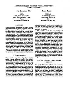
In order to quantify the informational value, the best choice is to know the application of the network. Since sensor networks have many applications, the informational value may change for each one. One of the methods used to quantify the information is count-based measure. The number of aggregated sensor readings in a packet is used as a countbased measure to quantify the information value. When a sensor 1 sends a data measure to a sensor 2, the informational value V is one. If the sensor 2 aggregates in the packet another measure, the informational value will be two. If the sensor 2 only retransmits the data sent by sensor 1 to the next node, the informational value remains the same (one). At each data aggregation the value V is increased by one unit. This was the approach used in [6] and [7] to evaluate V. In this section a novel method is proposed to evaluate the informational value using coverage area. The informational value using count-based measure has some disadvantages. If the sensors are randomly distributed in a region, some areas may be observed by many sensors and others by few sensors. Fig. 1 shows a network scenario where the sensors are not uniformly distributed. The network is formed by eight sensors, but five sensors cover a small area and only three sensors cover another larger region.
be applied when V is high and less or none error control will be applied for low V. The value of the probability pk will be closer to 1 (one) when a low variation in the measured quantity occurs and closer to 0 (zero) when great variation in the measured quantity occurs. The informational value Vk increases when the value of probability pk decreases. Thus, it will be higher when the variation in the value of physical quantity in the kth measure is high. III.
SIMULATION MODEL
The data packet of the link layer is the communication unit between the sensor nodes of the network. It contains a header with h bits, a trailer with tr bits and a payload with d bits of data. The payload also contains a 16 bit CRC code for error detection. The return packet used to acknowledge the transmission has the same format, but without the data. A received packet is not accepted when any of the five events happens: (A) the header of the received packet is corrupted; (B) the destination fails to synchronize with the trailer of the received packet; (C) the data of the received packet are corrupted after the channel code, if any, is decoded, causing the CRC check to fail; (D) the header of the return packet is corrupted and (E) the source is unable to synchronize with the trailer of the return packet. It is being assumed that the errors are statistically independent. The header is properly received if all the bits are correctly received: h (3) P[ A ] = 1 − p (γ f ) ,
[
Figure 1. Network with sensors unequally distributed
If the count-based measure was used, the left side of the network of Fig. 1 would contribute with more information. However, this is not true, since the right side covers a larger region with less sensors and this might be considered in the informational value. One option for this problem is to measure the value V based on the area observed by the sensors. The proposal in this section to the evaluation of V is to use the concept of spatial density, defined by the number of sensors ns in a given area A:
n ds = s . A
]
where p(γf) is the bit error probability of the forward channel for a given instantaneous signal-to-noise ratio (SNR) and γf denotes the instantaneous SNR of the forward channel. The
(1)
The informational value Vk of the kth measure of a sensor is given by: 1 (2) Vk = . ds For instance, consider a region with 100 m2 being monitored by 50 sensors. The total area is divided in smaller sub-areas that are monitored by a determined number of sensors. If the sub-area 1 with 20 m2 is covered by 5 sensors: ds1=ns1/A1=5/20=0.25 sensors/m2. A sub-area 2 with 15 m2 monitored by 20 sensors has ds2=ns2/A2=20/15=1.33 sensors/m2, and so on. The higher the number of sensors covering an area, the higher will be the spatial density and lower will be the value of V. A more robust error control will
event A indicates the complement of event A and P[A] is the occurrence probability of event A. The forward channel is used to send data packets and the reverse channel used to send ACK packets, indicating the success or not of the transmission. Since the ACK packet also has a header of h bits, the probability for event D has the same form: h (4) P [ D ] = [1 − p (γ r ) ] ,
where p(γ r ) is the bit error probability of the reverse channel. The events B and E occur if any bits of the synchronization trailer are received with errors: t (5) P [ B ] = 1 − p (γ f ) r
[
]
t (6) P [ E ] = [1 − p (γ r ) ] r The most probable error is that defined by event C, which occurs when any of the data bits are received with error:
[
]
[
] [
d (7) P [ C ] = 1 − p (γ f ) , For packets protected by an error correcting code, the probability of event C is evaluated considering the error correction capacity of the code. For a BCH (n,k,t) code capable of correcting up to t errors in a code word: t n k n−k P [ C ] = ∑ ⋅ p (γ f ) ⋅ 1 − p (γ f ) . (8) k k =0
]
The bit error probability p (γ ) depends of the modulation used by the nodes in the transmission. In this work is being assumed that the sensor nodes have OQPSK (Offset Quadrature Phase-Shift Keying) modulation. This modulation is used in the IEEE 802.15.4 standard for wireless sensor networks. Then, the bit error probability for the OQPSK modulation is given by [12]: (9) p (γ ) = Q 2γ ,
energy, where each transmitted bit consumes 1 unit of energy and each received bit consumes 0.75 units of energy: (16) E / E b = H .n pac (nbits + nbits 0.75 + E DEC / E b ), where nbits is the total number of bits of a packet, including the access code, header and payload. On the other hand, for the packets with ARQ the energy E/ Eb is the total number of bits transmitted and received, including the retransmissions: E / Eb = H.n pac [nbits + nack + (nbits + nack )0.75 + EDEC / Eb ], (17)
where Q (x ) :
where nack is the total number of bits of the return packet. The energy Edec/Eb for a BCH code (n,k,t) with m memories can be evaluated using the number of instructions needed for the microprocessor to execute the decoding process [2]. The number of instructions ninst is given by [2]: n inst = kt ( t + 1) m + 2 tm + (( k + 2 ) t ( t + 1) + ( 3t − 2 ) n + (18)
( )
− u2 (10) du. 2 2π x Thus, the packet error probability of the forward channel, PERf, and reverse, PERr, can be defined as: Q( x ) =
1
∞
∫ exp
∞
PER f = 1 − ∫ f (γ f ) P[ A] P[ B] P[ C] dγ f ,
(11)
0
∞
PER r = 1 − ∫ f (γ r ) P[ D] P[ E] dγ r ,
(12)
0
where f(γf) and f(γr) are the probability density functions and γf and γr are the SNR of the forward and reverse channels, respectively. The wireless channel is modeled using the Rayleigh fading, whose probability density function is given by: γ 1 (13) f (γ ) = exp − , for γ ≥ 0 γ γ where γ is the average received SNR. The error probabilities of each packet can be evaluated using equation (13) in (11) and (12). It is assumed that the propagation conditions between the transmitter and the receiver are the same in both directions. The reliability R is the normalized throughput, given by the percentage of the sent packets being delivered correctly to the sink node and it may be evaluated as: (14) R = [(n pac − nerror ) / n pac ], where npac is the total number of transmitted packets originated by a sensor node and nerror is the number of packets received with errors at the sink node. Since no specific hardware is being used, the energy consumption in the transmission and reception of the packets is expressed only in normalized terms. Only the energies consumed in the communication (transmission and reception) process and decoding process are considered. The energy spent in the encoding process is considered to be negligible, since it is a simple task and consumes less energy than the decoding process [6] [10]. The same model of [6] is considered, where the energy consumed per bit (Eb) is constant and the reception of a determined number of bits consumes approximately 75 per cent of the energy spent to transmit the same number of bits. The minimum energy consumed Emin/Eb for H hops is evaluated for a packet without error control: (15) E min / E b = H .n pac (nbits + nbits 0.75 ), where nbits is the total number of bits of a packet with no error control. The total energy consumed E/Eb in a sensor network for a packet with FEC and without ARQ corresponds to the total number of bits transmitted and received and the decoding
2 ( t + 1)( t + 3 )) + ( kt (t + 1) + ( 3t − 2 )( n − 1) + 2 t ( t + 1))
The consumed energy in the transmission of a bit is many times higher than the consumed energy used by the processor to execute one instruction [9], [10]. In this paper the parameters of [11] are considered, where the energy to transmit one bit is approximately 2 700 higher than the energy spent to execute one instruction. Thus, the decoding energy is: n (19) E dec / E b = inst 2700 IV.
ADAPTIVE ERROR CONTROL
A different error protection will be chosen for the message according to the informational value V. When the value of V is high, a strong error correction has to be used. There is a relation between the informational value and the chosen protection V → P (V). The problem is how to do this mapping, since the properties of P are unknown. Using a function could be a solution. This function would receive as input parameter the value V and would return the protection value P, indicating that a code capable of correcting P errors has to be used, for instance. However, finding an adequate function that would lead to an optimum efficiency is not an easy task [7]. Another option is to use a table for the mapping V → P (V). For each value or range of values V, a specific error protection is applied. This is the approach used in this paper to choose the appropriate error control. Each application may have a different table. Before sending data, the sensor node evaluates the informational value V and finds in the table the corresponding protection P. This is the error control to be applied in the packet. FEC and ARQ are the two basic categories of error control techniques. ARQ is simple and achieves reasonable throughput levels if the error rates are not very large. However, ARQ leads to variable delays which are not acceptable for real-time applications. FEC schemes maintain constant throughput and have bounded time delay. However, the decoding error rate rapidly increases with increasing channel error rate. In order to obtain high system reliability, a variety of error patterns must be corrected. Then a powerful
long code is necessary, which imposes a high transmission overhead. For the adaptive error control using informational value for area-based measures, three different regions were defined: 1) High density region: ds ≥ 1 sensors/m2; 2) Normal density region: 0.5 < ds < 1 sensors/m2; 3) Low density region: ds ≤ 0.5 sensors/m2. Each data packet originated by a sensor of a different region will have a different error control, based on the spatial density ds. Based on spatial density ds, the informational value V can be evaluated. Three adaptive schemes are proposed, using ARQ, BCH codes and hybrid FEC/ARQ, as shown in Table I. For the BCH code, the higher the value V the higher will be the error correcting capability t. For an ARQ system, the number of retransmissions increases for higher informational values. In order to find the table for mapping V → P (V), several simulations were made with different values of t (1-10) and number of retransmissions (1-10). The results were analyzed and the adaptive schemes being improved based on these results, until achieve the schemes of Table I. Table I. Adaptive error control
Error Control Informational value
V≤1 1