sion of the Cartesian space for robot i (nx) can be smaller than nq. Therefore, assuming that Ji has full row rank, the joint velocity vector Ëqi can be decomposed ...
Proceedings of the 2004 IEEE International Conference on Robotics & Automation New Orleans, LA • April 2004
Adaptive Force-motion Control of Coordinated Robots Interacting with Geometrically Unknown Environments Mehrzad Namvar and Farhad Aghili Canadian Space Agency 6767 route de l’Aeroport, St. Hubert Quebec, J3Y 8Y9, Canada mehrzad.namvar (farhad.aghili)@space.gc.ca
Abstract— Most studies on adaptive coordination of multirobot systems assume exact knowledge of system kinematics and deal with dynamic uncertainties. However, many industrial applications involve tasks in which a multi-robot system interacts with geometrically unknown environments. In this paper we consider a multi-robot system grasping a rigid object which is in contact with a frictionless surface with unknown geometry. The proposed adaptive hybrid force-motion controller guarantees asymptotic tracking of desired motion and force trajectories while ensuring exact identi£cation of tangential and normal directions to the constraining surface without persistency of excitation condition. The control signal is smooth and no projection is used in parameter update law. A simulation example is presented to illustrate the results.
I. I NTRODUCTION Coordination of multiple robots is essential in many applications such as manufacturing and assembly tasks which often include the situations where multiple arm robots are grasping an object in contact with environment, as shown in Fig.1. Examples are scribing, grinding, contour following and plotting. The purpose of controlling the coordinated system is to control the contact force between the environment and object in the constrained direction and the motion of the object in unconstrained directions, while maintaining internal forces that do not contribute to system motion to desired values. Several approaches in the literature have been proposed to address robot coordination problem. In [1], [15] a master/slave approach was considered where position of master robot was controlled and slave robots were under force control to maintain kinematic constraints. A linear system approach to the problem was considered in [16], [21]. The concept of internal force space was introduced by [9] and the relationship between the load distribution in object and internal forces was further explored in [17]. Force-motion setpoint problem for multiple robots was studied in [19] and the tracking problem was analyzed in [12] and [20] in the case of environmental constraints. To deal with uncertainty in system dynamics, adaptive controllers were proposed in [5], [18] where measurement of joint accelerations was used. This requirement was relaxed later in [6] and [7]. In [23] a systematic adaptive control
0-7803-8232-3/04/$17.00 ©2004 IEEE Canadian Crown Copyright
strategy based on the concept of virtual decomposition was introduced to handle a variety of control objectives. An adaptive synchronized control approach was presented in [14] to address the coordination problem when the robots are not kinematically constrained but perform a common task. Most adaptive schemes on robot control deal with uncertainty in system dynamics and assume that exact kinematics of interconnected system is known. However, in practice, due to imperfect knowledge of system parameters, the uncertainty in system kinematics can affect system stability and performance. In general, kinematic uncertainty is translated into uncertainty in robot Jacobian matrix or object Jacobian matrix. If the object is in contact with unknown and rigid environment, then kinematic uncertainty is translated into uncertainty in constraint Jacobian matrix. The uncertainty in robot Jacobian matrix was addressed in [2] for setpoint position control of a single arm robot in free space. The proposed PD controller with gravity compensation used an approximate nominal Jacobian matrix and included a saturation term making it robust against kinematics uncertainty. However, uncertainty in environment geometry which corresponds to uncertainty in constraint Jacobian matrix, has not been addressed in the literature so far. This problem arises in many applications such as scribing or grinding in which the motion of scriber or grinder on the surface together with the contact force are to be controlled while exact knowledge of contacting surface geometry is not usually available due to complexity of surface geometry or possible change in location and orientation of surface. In this paper we consider a multi-arm robot system manipulating an object in contact with a frictionless surface described by a smooth manifold which contains unknown parameters. The proposed adaptive control law estimates the unknown parameters and controls object motion and contact force between object and the constraining surface, while maintaining the internal forces to desired levels. Asymptotic convergence of force-motion errors to zero is guaranteed and it is shown that the error in estimation of constrain Jacobian matrix converges to zero without any persistency of excitation requirement. Moreover, the control signal is smooth and no projection is
3061
used in parameter update law. The proposed method also exploits redundancy in robot kinematics in order to keep the overall interconnected system in desired con£gurations during its operation. q22
where τi ∈ Rnq is the vector of joint torques and fi ∈ Rnx denotes the interacting force between robot end-effector and the object. The inertia matrix Mi ∈ Rnq ×nq is assumed to be a bounded and positive de£nite matrix. C i q˙i ∈ Rnq represents the Centrifugal and Coriolis forces and gi ∈ Rnq is a bounded vector representing gravitational forces. It is assumed that M˙ i − 2Ci is skew-symmetric [3]. Due to possible redundancy in robot kinematics, the dimension of the Cartesian space for robot i (nx ) can be smaller than nq . Therefore, assuming that Ji has full row rank, the joint velocity vector q˙i can be decomposed by [4], [11] q˙i = Ji+ Ji q˙i + Ji− q˙i
(3)
where Ji+ = JiT (Ji JiT )−1 and Ji− = I −Ji+ Ji . Since Ji Ji− = 0, it is clear that Ji− q˙i belongs to the null space of Ji and thus it has no effect on robot end-effector velocity x˙ i . This redundancy in robot kinematics can be exploited to specify desired joint trajectories qid that allow each robot to avoid reaching singular con£gurations or to maintain distance from its joint limits while keeping its task space motions unaltered [3]. B. Constraining surface Let xt ∈ Rnx with nx ≤ 6 be the vector of position and orientation of the object tip which is in contact with a frictionless environment. We assume that xt is decomposed by � � χ (4) xt = η
x1
xo
F
χ
Robot 1
q12
Object tip
q11 χ 2
q21
d0
Fig. 1.
(2)
x2
Robot 2
l
A. Robot dynamics
qi + Ci (qi , q˙i )q˙i + gi = τi − JiT fi Mi (qi )¨
f1
y0
We consider m robots (possibly redundant) grasping tightly a rigid object at m speci£ed points such that there is no relative translational motion between the end-effectors of robots and the object. We assume that all positions and orientations are represented with respect to the world frame denoted by Ow . It is assumed that one point of the object, denoted by object tip, is kinematically constrained by a rigid and frictionless environment.
where Ji (qi ) ∈ Rnx ×nq with nx ≤ nq is the robot Jacobian matrix. The dynamics of ith robot is described by
η
f2
II. D ESCRIPTION OF INTERCONNECTED SYSTEM
It is assumed that each robot grasps the object at its endeffector whose vector of position and orientation is denoted by xi ∈ Rnx . Denoting qi as the vector of joint angles of robot i, robot end-effector velocities are related to joint angle velocities by Ji (qi )q˙i = x˙ i (1)
q13
χ3
q23
0
x0
d0
A two-robot interconnected system in R2
where χ ∈ Rnχ denotes those components of xt that are constrained by a nχ − nφ dimensional manifold φ(χ, θ) = 0 ∈ Rnφ
(5)
with nφ < nχ . Also, η ∈ R denotes the unconstrained components of xt . For example, in the interconnected system shown in Fig. 1, χ ∈ R2 represents the Cartesian position of object tip and the angle η ∈ R1 represents object orientation. The parameter vector θ is assumed to be unknown but constant and it belongs to a compact parameter set Ω. Differentiating (5) with respect to time and de£ning the constraint Jacobian matrix J ∈ Rnφ ×nχ by nη
J (χ, θ) := κ(χ, θ) where κ(χ, θ) := �
∂φ(χ, θ) ∂χ
∂φ(χ, t) −1 � , ∂χ
(6)
(7)
yields J (χ, θ)χ˙ = 0. The scalar valued function κ(χ, θ) is a measure of the curvature of the constraining surface at χ. Note that with this de£nition, the constraint Jacobian matrix J has unit Euclidian norm. The velocity vector χ˙ belongs to the nχ − nφ -dimensional plane St which is tangential to the constraining surface at χ, as shown in Fig. 2. It is known that the tangential plane speci£es the null space of J , i.e. S t = null(J ). Equivalently, rows of J span the nφ -dimensional orthogonal complement of St denoted by St⊥ [4]. We de£ne the matrix P(χ, θ) as the orthogonal projection onto St P(χ, θ) := I − J T (J J T )−1 J which indicates that for any vector y in Rnχ , Py ∈ St and (I − P)y ∈ St⊥ . Obviously, since χ˙ belongs to St , its orthogonal projection onto St is χ˙ itself
3062
P(χ, θ)χ˙ = χ˙
(8)
If θˆ denotes the estimate of parameter vector θ, then the ˆ estimated constrained Jacobian matrix is denoted by Jˆ(χ, θ). ˆ Due to the mismatch between J and J , the constrained velocity χ˙ does not necessarily belong to null(Jˆ), indicating that the projection of χ˙ onto null(Jˆ) differs from χ˙ or ˆ χ˙ �= χ. ˆ P(χ, θ) ˙ Therefore, in order to have a measure of mismatch between J and Jˆ, we de£ne velocity projection error by (9) eχ := Pˆ χ˙ − χ˙ which can be evaluated through measurements (See Fig. 2). 1) Constraint motion: Obviously, for the unconstrained component η, one can specify any reference trajectory ηd without knowing J . However, in case of constrained component χ, one needs to know the geometry of constraining surface in order to be able to specify a desired trajectory χd . It is then reasonable to specify a desired velocity trajectory χ˙ d and expect that the object tip velocity χ˙ tracks the image of χ˙ d on the tangential plane St ; or equivalently χ˙ → P χ˙ d . Since in this case only the velocity vector χ˙ is controlled, we make the following assumption: Assumption 1: The set of all constrained coordinates reachable by the object tip, de£ned by � � S := χ : φ(χ, θ) = 0, θ ∈ Ω (10) is bounded. 2) Contact force: Since the object tip is constrained by environment, the force F ∈ Rnχ is exerted to the object tip at the contact point. The contact force belonging to St⊥ can be expressed in terms of a nφ -dimensional vector denoted by Lagrange multiplier λ F = J (χ, θ)T λ
(11)
which by orthonormality of J implies �F � = �λ�
(12)
In standard hybrid force-motion control where J is assumed known, control of contact force is achieved by specifying a desired trajectory λd (t) and controlling λ. Given the measured force F , the value of λ(t) used in control law can be calculated from (11). However, when geometry of the constraining surface and consequently J are unknown, computation of λ(t) from measured F is not straightforward. In addition, it is not obvious in this case how the speci£ed λ d (t) is interpreted in terms of a desired force Fd (t). To resolve these concerns, it is necessary to relax the problem in such a way that a direct relationship between F and λ can be established without knowing J . For this purpose, in the sequel we consider the following assumptions. Assumption 2: i) dim St⊥ = 1, ii) The constraining surface belongs to a class of differentiable manifolds described by φ(χ, θ) := χ3 + h(χ1 , χ2 )θ + b = 0 3
(13)
where χ = [χ1 χ2 χ3 ] ∈ R is the Cartesian position of object tip and h(χ1 , χ2 ) is a known and continuously differentiable function on R×R, and b is a constant scalar, T
f1 Robot 2
Robot 1
F
Estimated tangential plane
x1 f2
x2
xo
Tangential plane
Object tip
Fig. 2.
Object and constraining surface
iii) For any θ ∈ Ω and χ ∈ S, 0 < κ ≤ κ(χ, θ) where κ is a known scalar. According to Assumption 2-i, λ is a scalar and J is a gradient vector perpendicular to the constraining surface at χ, and pointing towards the surface φ(χ, θ) = where > 0. By Assumptions 2-i and 2-ii, it is possible to establish a unique relationship between λ and F without any need for knowing the geometry of constraining surface. Notice that by the assumption, the constraint Jacobian matrix becomes (14) J T = κ(χ, θ)(Eθ + ν) �T � � �T ∂h ∂h 0 where E := , ν := 0 0 1 and ∂χ1 ∂χ2 κ(χ, θ) = �Eθ + ν�−1 . If F3 is the components of F along χ3 axis then by virtue of (11), it is inferred that F3 = κλ which in view of (12) implies that λ = �F � sgn(F3 )
(15)
Therefore, the relationship between Lagrangian multiplier and F is established without knowing J and besides, λ is computable from measured F . Moreover, it is possible now to establish a meaningful relationship between λd and Fd which must satisfy (15). As an example, consider the case where the object is known to be located always above the constraining surface or in a subset of R3 speci£ed by Φ + := {χ | φ(χ, θ) > 0, ∀θ ∈ Ω}. Then, at each instant of time, the magnitude of λd (t) determines the desired magnitude of force signal Fd (t). Also, the sign of λd (t) determines whether Fd (t) is a pulling or pushing force with respect to the surface, e.g. a pushing force corresponds to a negative value of λd (t). Assumption 2-iii is mainly for technical reasons and indicates that the slope of constraining surface along χ3 axis is £nite for all χ ∈ S. 3) Force projection error: A new concept similar to velocity projection error in (9) can be introduced as force projection error (16) eF := J˜T λ = JˆT λ − F which is also a measure of mismatch between Jˆ and J and it can be calculated from measurements. The difference between velocity and force projection error is that in the former the error in constraint Jacobian J˜ is measured by means of velocity signal while in the latter the error is measured through using force signal (See Fig. 2). From implementation point of
3063
view, the use of velocity signal is advantageous since it is normally less noisier than force signal. However, as discussed in sections III-C and III-D, convergence of eF is stronger than that of eχ in a sense that convergence to zero of eF is suf£cient for convergence to zero of �J˜�, but only in particular cases convergence of eχ implies convergence of �J˜�. This fact indicates that for identi£cation of constraining surface geometry, force signal is more informative than velocity signal. C. Identi£cation of environment geometry Before proceeding further, it is worthwhile here to discuss the necessity of an adaptive approach to the problem. First, notice that force signal F can be used to determine the projection matrix P at any instant of time. In fact, since F is an element of St⊥ and P projects any vector in Rnχ onto St , then the projection matrix can be determined from F as follows FFT P(χ, θ) = I − (17) �F �2 One may now wonder if the projection matrix is already known from (17), why it should be estimated through identi£cation of θ. The answer to this question relies on the fact that in most hybrid force-motion control methods in literature [11], [10], [6], [22], [23] the derivative of projection or Jacobian matrices are used in control design. Obviously, when geometry of constraining surface is known, one can simply differentiate P(χ, θ) and express P˙ in terms of χ˙ and θ. However, when θ is unknown, calculation of P˙ through (17) will involve computation of force derivative F˙ . The necessity of an adaptive approach to the problem then becomes obvious since in this approach and in the control signal, P˙ is replaced d ˆ ˆ whose computation does P(χ, θ) by the estimated matrix dt ˙ not require knowledge of F . 1) Notations: Before proceeding into description of other system components, some notations and de£nitions are introduced. De£ning the estimated Jacobian by JˆT := ˆ θˆ+ ν), the error in Jacobian matrix can be expressed κ ˆ (χ, θ)(E by ˆ θ˜ + κ ˆ (χ, θ)E ˜ Eθ + κ ˜ν (18) J˜T = κ ˆ − κ(χ, θ). The augmented constraint where κ ˜ = κ ˆ (χ, θ) Jacobian matrix Jt is constructed from J as � � Jt := J 01×nη (19) which clearly implies that Jt x˙ t = 0. The estimated augmented Jacobian Jˆt can be de£ned in an obvious way. For simplicity ˆ + = JˆT (JˆJˆT )−1 . We in notation, we de£ne Tˆ := [Jˆ(χ, θ)] also de£ne the augmented matrices Pˆ and Tˆ as � � � � Pˆ 0 Tˆ ˆ ˆ P := and T := (20) 0 Inη 0nη ×1 Also, P and T are de£ned similarly. The augmented velocity and force projection errors are de£ned by � � � � eχ eF e¯χ := , e¯F := (21) 0nη ×1 0nη ×1
Obviously, each variable has the same magnitude as its augmented variable. Also, all projection matrices such as P are idempotent i.e. P 2 = P . D. Object dynamics The object is assumed to be a rigid body contacting at m distinct points, xi , with end-effector of robots. The coordinate of object center-of-mass is denoted by xo ∈ Rnt and it is assumed that x˙ o and object tip velocity vector x˙ t are related by (22) x˙ o = R(xt )x˙ t where R(xt ) ∈ Rnt ×nt is assumed invertible. Also, x˙ i and x˙ o are related by x˙ i = Ai (xo )x˙ o , i = 1, ..., m
(23)
where Ai ∈ Rnx ×nt is the object Jacobian matrix. The dynamics of object is then described by xo +Co (xo , x˙ o )x˙ o +go = Mo (xo )¨
m
ATi fi +R−T JtT λ (24)
i=1
where Mo ∈ Rnt ×nt denotes the inertial matrix assumed to be bounded and positive de£nite. C o ∈ Rnt ×nt is the Coriolis and Centrifugal matrix, and go ∈ Rnt represents the vector of gravitational forces. Both Co and go are assumed to be bounded and in addition M˙ o − 2Co is skew-symmetric. De£ning the augmented object Jacobian matrix as AT = [AT1 , ...., ATm ] ∈ Rnx ×mnt and the interacting force vector by T T ] ∈ Rmnt f = [f1T , ..., fm
then we can decompose f as f = A+T AT f + A− f
(25)
where A+T = A(AT A)−1 , and the projection matrix A− is de£ned by A − = I − AA+T . Observing that AT A− = 0, it is inferred that A− f lies in the null space of AT and thus it does not contribute on the motion of object. The force component A− f is commonly called in literature as the internal force [9], [17]. The internal forces can contribute in internal strain buildup in the object. By specifying some desired force trajectories such as fd , the internal forces can be effectively controlled in order to provide e.g. suf£cient friction forces in the contact points between the object and robots [13]. III. S YNTHESIS OF CONTROL LAW We start the synthesis of the control law by constructing the overall system dynamics. First, we notice that in view of (25) and the object dynamics (24), the interacting force between the robot i and object, can be calculated by [6] ¨o + Co x˙ o + go − R−T JtT λ) + (A− )i f (26) fi = (A+T )i (Mo x
3064
where (A+T )i and (A− )i ∈ Rnx ×nt are obtained by partitioning A− and A+T as (A+T )1 (A− )1 .. .. − A+T = , A = . . (A− )m (A+T )m An important property of A− which will be used later is �m T − that i=1 Ai (A )i = 0. Incorporating (26) in the robot dynamics (2) gives the complete dynamical equations of the interconnected system ¨o + Co x˙ o + go − R−T JtT λ) Mi q¨i + Ci q˙i + gi + JiT (A+T )i (Mo x +JiT (A− )i f = τi
and sqi := q˙i − vqi , sλ := Gλ ∗ (λ − λd ) where Gλ (s) is any stable and stably invertible transfer function such that sGλ (s) is proper. As an example consider the transfer function s+a1 where a1 , a2 > 0. Note that Gλ (s) and Gλ (s) = s(s+a 2) Gf (s) are such that the computation of s˙ λ and s˙ f , used in control signal, does not involve knowledge of force derivatives λ˙ and f˙, respectively. A. Control signal Based on signal error descriptions in the last section a new composite error signal can be de£ned by s := Pˆ sx + β Tˆsλ − e¯χ
(27)
To see which terms in (27) should be controlled and which terms can be cancelled by the control torque τi , we will project ¨o onto orthogonal spaces determined by the q˙i , q¨i , x˙ o and x Jacobian matrices Ji and Jt [11]. Therefore, in view of (4) and (9), we can decompose object tip velocity and acceleration ¨t as follows vectors x˙ t and x x˙ t = Pˆ x˙ t − e¯χ
(28)
where β is a positive scalar. The composite error signal represents the error in object tip force and motion, and consists of two orthogonal terms Pˆ sx and β Tˆsλ − e¯χ . In view of the signal decompositions speci£ed by (29), (30), (32) and (32), and signal error de£nitions, we consider the following control law Mi ari + Ci vir + gi +JiT (A+T )i [Mo aor + Co vro + go − R−T (JˆtT λ − u)]
τi =
˙ x ¨t = Pˆ x ¨t + Pˆ x˙ t − e¯˙χ
−Li (Ji+ Ai Rs + Ji− sqi + γJiT (A− )i sf ) d −Mi (Ji+ Ai R)s − Mi J˙i− sqi dt ˙ + JiT (A− )i f −JiT (A+T )i Mo Rs
where e¯χ and Pˆ are given by (21) and (20), respectively. Then, by virtue of (22) we obtain x˙ o = R(Pˆ x˙ t − e¯χ )
(29)
˙ x ¨o = R(Pˆ x ¨t + Pˆ x˙ t − e¯˙χ ) + R˙ x˙ t
(30)
Similarly, q˙i and q¨i can be decomposed as q˙i
(3)
(1)
Ji+ Ji q˙i + Ji− q˙i = Ji+ x˙ i + Ji− q˙i
(23)
Ji+ Ai x˙ o
= =
q¨i
+
(29) Ji− q˙i =
(31)
Ji+ Ai R(Pˆ x˙ t
�
− e¯χ ) + ��
˙ = Ji+ Ai R(Pˆ x ¨t + Pˆ x˙ t − e¯˙χ ) + Ji− q¨i � �� � + ˙ ˙ ˙ +J (Ai Rx˙ t + Ai x˙ o − Ji q˙i ) i
vir
:=
ari
:=
vro
:=
aor
:=
�
The general idea behind this decomposition is to compensate all underbraced terms while cancelling the remaining terms. For this purpose we de£ne the following signals that will be used in the control law: � � χ˙ d vx := η˙ d − Λη η˜ where χ ˜˙ = χ˙ d − χ, ˙ η˜ = η − ηd and Λη is an arbitrary positive de£nite matrix. Also, v qi := q˙id − Λq q˜i where q˜i = qi − qid with Λq as an arbitrary positive de£nite matrix. Similarly the force error signal is de£ned by s f = Gf ∗ f˜ where f˜ = f − fd and Gf (s) is any stable and strictly proper low-pass transfer a where a > 0. The notation ∗ function such as Gf (s) = s+a stands for convolution operator. Moreover, we de£ne the error signals sx , sqi and sλ by � � χ ˜˙ sx := x˙ t − vx = ˙ (33) η˜ + Λη η˜
(35)
where Li are arbitrary positive numbers and
Ji− q˙i
(32)
(34)
Ji+ Ai R(Pˆ vx − β Tˆsλ ) + Ji− vqi − γJiT (A− )i sf � � Ji+ Ai R Pˆ v˙ x + Pˆ˙ vx − β d (Tˆsλ ) + Ji− v˙ qi dt d T − + −γ (Ji (A )i sf ) + Ji (Ai R˙ x˙ t + A˙ i x˙ o − J˙i q˙i ) dt R(Pˆ vx − β Tˆsλ ) � � R Pˆ v˙ + Pˆ˙ v − β d (Tˆs ) + R˙ x˙ t (36) x
x
dt
λ
with γ > 0. The auxiliary control signal u used for convergence of eχ and eF will be determined later. It can be veri£ed that the control signal τi depends on position, velocity and force signals f and F . Here for simplicity in presentation we have assumed that system dynamic variables Mi , Ci , gi , Mo , Co and go are known. B. Error dynamics Substituting for τi in system dynamics (27) it is possible to show that the error equation is ultimately expressed in standard form by ¯ = −H T + R−T (J˜T λ − u) Meq r˙ + Ceq r + Lr t
(37)
¯ + (H + )T Mo H + and Ceq = C¯ + where Meq = M + T + (H ) Co H + (H + )T Mo (H˙+ ) where H is given by T T ] with Hi = Ji+ Ai . Also, the PseudoH = [H1T , ..., Hm inverse of H is de£ned by H + = (H T H)−1 H T and
3065
¯ = diag(M1 , ..., Mm ), C¯ = diag(C1 , ..., Cm ) and L ¯ = M diag(L1 , ..., Lm ). The error signal ri is de£ned by ri = Hi Rs + Ji− sqi + γJiT (A− )i sf
(38)
r = [r1 , ..., rm ]T and sq = [sq1 , ..., sqm ]T . An important property of the error equation (37) is that Meq and Leq are positive de£nite and in addition M˙eq − 2Ceq is skewsymmetric. C. Design of auxiliary control signal u In the sequel, we will construct the auxiliary control signal u to ensure convergence of e¯F . We start the design procedure by noticing that the RHS term in the error equations (37) ˜ depends on J˜tT which in turn depends on parametric error θ. From (18), the error in augmented Jacobian vector is given by ¯ +κ J˜tT = κ ˆ E¯θ˜ + κ ˜ Eθ ˜ ν¯ (39) � � � E ν where E¯ = , ν¯ = . Note that the 0nη ×nχ 0nη ×1 ˜ due to the Jacobian error is not linear in parameter error θ, presence of κ ˜. To start the design, we consider the following Lyapunov function 1 1 V1 = rT Meq r + θ˜T θ˜ 2 2 whose derivative along (37) becomes �
˙T ¯ − sT λ(ˆ ¯ +κ κE¯θ˜ + κ ˜ Eθ ˜ ν¯) + θ˜ θ˜ + sT u V˙ 1 = −rT Lr where in deriving V˙ 1 we have used Lemma ??-iii, (39) and the fact that M˙eq − 2Ceq is skew-symmetric. Consider now the parameter adaptation law ˙ κλE¯T P e¯F (40) θˆ = κ ˆ λE¯T s − cˆ where c is a positive number to be determined later. Note that P can be constructed from P as (20) and P is computable from F by (17). The £rst term in the parameter adaptation law is a standard gradient term while the second term is to ensure convergence of eF to zero. Incorporating (40) into V˙ 1 yields ¯ − sT λ˜ ¯ + ν¯) − cˆ V˙ 1 = −rT Lr κ(Eθ κλ¯ eTF P E¯θ˜ + sT u The second term in RHS of the above equality depending on κ ˜, is considered as perturbation and its effect will be compensated by u. The term cˆ κλ¯ eTF P E¯θ˜ can be further simpli£ed by replacing for κ ˆ E¯θ˜ from (39) ¯ + ν¯)) cˆ κλ¯ eTF P E¯θ˜ = cλ¯ eTF P (J˜tT − κ ˜ (Eθ P JtT
= 0 and κ is a scalar, then it results that However, since ¯ + ν¯) = 0 and hence, cˆ eTF P JˆtT . On the P (Eθ κλ¯ eTF P E¯θ˜ = cλ¯ other hand, multiplying (16) by P and recalling that PF = 0, yields P e¯F = P JˆtT λ. Therefore, we conclude that eTF P e¯F = c�P e¯F �2 cˆ κλ¯ eTF P E¯θ˜ = c¯ which £nally yields ¯ − c�P e¯F �2 − sT λ˜ ¯ + ν¯) + sT u V˙ 1 = −rT Lr κ(Eθ
The following lemma gives useful upperbounds for −�P e¯F �2 and |˜ κλ| expressed in terms of �¯ eF �. Lemma 1: Under Assumption 2, the following inequalities hold: i) |˜ κλ| ≤ �¯ eF � � 1 2 eF �2 . ii) �P e¯F � ≥ (1 − 1 − κ2 )�¯ 2 Using Lemma 1, V˙ 1 can be bounded by � ¯ c (1− 1 − κ2 )�¯ ¯ ν )�+sT u V˙ 1 ≤ −rT Lr− eF �2 +�s��¯ eF ��(Eθ+¯ 2 The next step is to determine u for compensating the effect of the positive term in V˙ 1 . First, notice that this term can be bounded by ¯ + ν¯)� ≤ 1 �s�2 (�E� ¯ 2 �θ�2 + 1) + 1 �¯ eF �2 �s��¯ eF ��(Eθ 2 2 where in deriving the previous inequality we have used the fact that for any scalars x and y, |x||y| ≤ 12 x2 + 12 y 2 . Moreover, ¯ and ν¯ are orthogonal and �¯ notice that Eθ ν � = 1. The effect 1 2 eF � can be readily compensated by choosing of 2 �¯ � c = 2(1 − 1 − κ2 )−1 (1 + Lf ) (41) where Lf is any arbitrary positive number. The problem now is reduced to compensate the effect of 1 2 ¯ 2 �θ�2 +1) by u. For this purpose we need a known �s� (�E� 2 bound for �θ�. To avoid this requirement, we will use an estimator to estimate �θ�2 , independently. Let ϑˆ stands for the estimate of �θ�2 and choose u as 1 ¯ 2ˆ u = − (�E� ϑ + 1)s (42) 2 ˆ 2 and ϑˆ are not necessarily identical since these Note that �θ� quantities are estimated by independent estimators. This yields 1 ˆ ¯ − Lf �¯ ¯ 2 (�θ�2 − ϑ) V˙ 1 ≤ −rT Lr eF �2 + �s�2 �E� 2 Now, introducing the new Lyapunov function V2 as 1 ˆ2 V2 = V1 + (�θ�2 − ϑ) 2 and the parameter update law 1 ˙ ¯ 2 ϑˆ = �s�2 �E� 2 it results that
¯ − Lf �¯ V˙ 2 ≤ −rT Lr eF �2
(43)
(44) (45)
Note that the additional parameter estimator (44) is £rst order and thus it does not increase signi£cantly the complexity of the overall controller. Its advantage is to relax the need for a priori known upperbound for �θ�. The following result can then be stated. Theorem 1: Consider the control law τi given by (35) together with the auxiliary control signal given by (42), and the parameter adaptation laws (40) and (44). Then, all error signals ˜˙ remain bounded and r, s, eF , eχ , �J˜�, Ji− sqi , (A− )i sf , P χ, ˜ η˜, λ and u converge to zero asymptotically.
3066
Proof: Boundedness of all signals and convergence to zero of r and e¯F follow from (45) and Barbalat’s lemma [8]. Convergence of s, Ji− sqi and (A− )i sf to zero follows from convergence of r and due to the orthogonality of three terms appearing in r. Similarly, orthogonality of the terms in s together with convergence to zero of e¯F (and consequently e¯χ and J˜t ), and the structure of Pˆ and sx , imply convergence to zero of signals as stated by the theorem. � Note that in force regulation case where λ converges to zero, convergence to zero of �J˜� does not necessarily follow from convergence of eF . In fact, in absence of contact force, eF is no longer informative for identi£cation of environment geometry and alternatively the velocity signal should be used as a source of information, as described in the next section. D. Convergence of eχ When λ does not converge to zero, convergence of �J˜�, and consequently eχ , follow from convergence of eF . However, it is possible to modify the control law and achieve convergence of eχ to zero, independently. This can improve system transient response specially for those instants of time where force signal is close to zero and computation of the projection matrix by (17) becomes numerically involved. Theorem 2: Consider the control law τi given by (35) together with the auxiliary control signal given by 1 ¯ 2ˆ u = − (�E� (46) ϑ + 1)s + α¯ eχ 2 and the parameter adaptation laws (44) and ˙ κλE¯T P e¯F + αβsλ κ ˆ E¯T x˙ t (47) θˆ = κ ˆ λE¯T s − cˆ Then, all results of Theorem 1 hold and in addition convergence of eχ to zero is achieved independently of the convergence of eF to zero. IV. S IMULATION EXAMPLE We consider two identical 3-DOF manipulators grasping a rigid object of triangular shape with equal sides of length 0.4m, as shown in Fig. 1. The base of each robot is located at a distance of d0 = 1.9071m from χ3 axis. For each robot the joint angle vector is de£ned by q i = [qi1 , qi2 , qi3 ]T . The length of all robot links are assumed to be l = 1m and the mass of each link is m = 1kg. We denote xi ∈ R2 as the Cartesian position of the end-effector of robot i. It is assumed that the orientation of object is not restricted at xi . The Jacobian matrices Ji and A, as de£ned before, belong to R 2×3 and R4×3 , respectively. The interacting force at xi is denoted by fi ∈ R2 . The object tip position χ = [χ2 , χ3 ] is assumed to be constrained by a second-order polynomial manifold described by φ(χ, θ) = χ3 − y0 + a(χ2 − x0 )2 = 0 The orientation of the object is represented by the angle η and it is assumed to be unconstrained. The constraint Jacobian matrix is expressed by J = κ(Eθ + ν) where � � � � 2χ2 −2 0 E= , ν= 0 0 1
�T � . The true values of parameters are and θ = a ax0 a = 2 and x0 = 0.2m. As initial guess, we have considered ˆ = a ˆ = 0.2 and x ˆ = 0.02m which corresponds to θ(0) � �T0 0.2 0.004 . It assumed that object tip is initially located � �T at χ(0) = 0 y0 where y0 = 1.4407m, and η(0) = 0o . The initial con£guration of robots are such that q 1 (0) = [90o 45o 45o ]T and q2 (0) = [90o − 45o − 45o ]T . The desired object orientation is de£ned as η d (t) = 10o (1 + sin 2πt) while the desired � translational �T velocity for object tip is speci£ed as χ˙ d (t) = sin πt 0 . Obviously, χ˙ d does not belong to the tangential plane St at any time. As a result, the controller makes the object tip velocity χ˙ converge to the image of χ˙ d on St . To control the contact force F , we de£ne λ d (t) = −20 + sin 4πt < 0 which in view of (15) indicates that the desired force Fd is a pushing force with respect to the constraining surface. Moreover, to regulate the internal forces to zero we consider fd (t) = 0 ∈ R4 , ∀t ≥ 0. Due the fact that the orientation of the object is not restricted at xi , the interconnected system has kinematic redundancy. Therefore, to keep the robots not far from their initial con£guration during the operation, we specify q1d (t) = q1 (0) and q2d (t) = q2 (0), ∀t ≥ 0. The following gains have been used in the control law: Λq = ¯ = 10I, Λη = 10, β = 100, α = 10, γ = −10 and 10, L 2 s+1 and Gλ = s(s+2) . c = 2.5. Moreover, Gf = s+2 Fig. 3 demonstrates convergence of error signals r, s and J − sq to zero. It is seen from Fig. 3 that torque control signals τ1 , τ2 and auxiliary control signal u are smooth and in addition, u converges to zero. Fig. 4 demonstrates ˜ and convergence of motion and force errors η˜, �P χ�, ˜˙ λ − �A sf �. Convergence of motion and force projection errors eχ , eF together with �J˜� are seen from Fig. 5. Note that parametric error, as seen in Fig. 5-d, does not convergence to zero. The convergence rate of eχ and eF are mostly affected by the gain c while convergence rate of composite error signal ¯ Evidently, high gains result in r is mainly determined by L. high picks in control signals. V. C ONCLUSION Convergence of force-motion errors in a coordinated system interacting with geometrically unknown environment has been shown. The error in constraint Jacobian matrix converges to zero without persistency of excitation condition. It is also straightforward to extend the results to the case where robot or object dynamics have uncertain parameters. R EFERENCES [1] S. Arimoto, F. Miyazaki, and S. Kawamura. Cooperative motion control of multiple robot arms or £ngers. IEEE Transactions on Robotics and Automation, 9(2):226–231, April 1993. [2] C.C. Cheah, M. Hirano, S. Kawamura, and S. Arimoto. Approximate jacobian control for robots with uncertain kinematics and dynamics. IEEE Transactions on Robotics and Automation, 19(4):692–701, August 2003. [3] C. Canudas de Wit, B. Siciliano, and G. Bastin. Theory of robot control. Springer-Verlag, London, 1996. [4] G.H. Golub and C. F. Van Loan. Matrix computations, Third edition. The Johns Hopkins University press, Baltimore and London, 1996.
3067
3
a
2
b
1 1
0
0.5
1
1.5
0
2 Robot 1 joint torque (N.m.)
Redundant joint space error
0
0.5
0.4 − ||J sq||
0.3 0.2 0.1 0
0.5
1
1.5
2
Robot 2 joint torque (N.m.)
Auxiliary control signal
0 2
u
1 0 −1 −2
0
0.5
1
1.5
2
0
0.5
1
1.5
2
50
0
0.5
1
1.5
2
150 τ
2
100 50 0 0
0.5
1 Time(s)
1.5
a
b Object−tip velocity error (m/s)
Object orientation error (deg.)
−2 −4 −6 −8 −10 −12
0
0.5
1
1.5
0.7 0.6 0.5 0.4 0.3 0.2 0.1 0
2
5 Internal force error index
0.1 Lagrangian error (N)
0 −0.1 −0.2 −0.3 −0.4 −0.5 0
0.2
0.4 0.6 Time(s)
0
0.5
−3
c
0.8
1
1
1.5
2
1.5
2
d
x 10
4 3 2 1 0
0
0.02
0
0.5
1
1.5
5
0
2
0
0.5
c
1 Time(s)
1.5
2
1.5
2
d
1.86 0.6 0.5 0.4 0.3 0.2
1.84
1.82
1.8
0.1 0
0
0.5
1 Time(s)
1.5
2
1.78
0
0.5
1
2
Fig. 3. Pro£les of composite error signals �r�, �s� and �J − sq � together with robot joint torques and auxiliary control signal u.
0
0.04
||e || F 10
Time(s)
Time(s)
2
0.06
1
−50 −100
0.08
0
τ 0
Estimation error in constraint Jacobian
2
15 ||eχ||
Force projection error (N)
1.5
Parametric error
||r||
Velocity projection error (m/s)
0.1
||s||
0.5
1 Time(s)
Fig. 4. a: Object orientation error η˜, b: Object-tip velocity error �P χ�, ˜˙ c: ˜ and d: Internal force error index �A− sf � Lagrangian error λ
[5] Y. R. Hu and A. A. Goldenberg. Dynamic control of multiple coordinated redundant robots. IEEE transaction on systems, man and cybernetic, 22:568–574, 1992. [6] J. H. Jean and L. C. Fu. An adaptive control scheme for coordinated manipulator systems. IEEE Transactions on Robotics and Automation, 9(2):226–231, April 1993. [7] J. H. Jean and L. C. Fu. Adaptive hybrid control strategies for constrained robots. IEEE Transactions on Automatic Control, 38:598– 603, April 1993. [8] H. K. Khalil. Nonlinear Systems. Prentice Hall, New Jersey, 1996. [9] K. Kreutz and A. Lokshin. Load balancing and closed chain multiple arm control. Proc. of ACC, pages 2148–2155, 1988. [10] Y. L. Liu and S. Arimoto. Adaptive and nonadaptive hybrid controllers for rheonomically constrained manipulators. Automatica, 34(4):483– 491, 1998. [11] R. Lozano and B. Brogliato. Adaptive hybrid force-motion control for redundant manipulators. IEEE Transactions on Automatic Control, 37(10):1501–1505, October 1992.
Fig. 5. Error in estimation of environment geometry: a: Velocity projection error �eχ �, b: Force projection error �eF �, c: Error in estimation of constraint ˜ Jacobian �J˜� and d: Parametric error �θ�
[12] N.H. McClamorch and R.H. Cannon. Feedback stabilization and tracking of constrained robots. IEEE Transactions on Automatic Control, 33:419–426, May 1988. [13] Y. Nakamura, K. Nagi, and T. Yashikawa. Dynamics and stability in coordination of multiple robotic mechanisms. International Journal of Robotics, 8(2), April 1989. [14] D. Sun and J.K. Mills. Adaptive synchronized control for coordination of multirobot assembly tasks. IEEE Transactions on Robotics and Automation, 18(4):498–509, August 2002. [15] J.M. Tao, J.Y.S. Luh, and Y.F. Zheng. Compliant coordination control of two moving industrial robots. Proc. IEEE Int. Conf. Robotics and Automation, pages 1407–1412, 1987. [16] T.J. Tarn, A.K. Bejczy, and X. Yun. Design of dynamic control of two cooperating robot arms: closed chain formulation. Proc. IEEE Int. Conf. Robotics and Automation, pages 7–13, 1987. [17] I.D. Walker, R.A. Freeman, and S.I. Marcus. Analysis of motion and internal loading of objects grasped by multiple cooperating manipulators. Int. J. Robotics Res., 10(4):396–409, 1991. [18] M.W. Walker. Adaptive control of manipulators containing closed kinematics loop. IEEE Transactions on Robotics and Automation, 6:10– 19, February 1990. [19] J.T. Wen and K.K. Delgado. Motion and force control of multiple robotic manipulators. Automatica, 28(4):729–743, 1992. [20] B. Yao, W. B. Gao, S.P. Chan, and M. Cheng. VSC coordinated control of two manipulator arms in the presence of environmental constrains. IEEE Transactions on Automatic Control, 37:1806–1812, Nov. 1992. [21] T. Yoshikawa and X.Z. Zheng. Coordinated dynamic hybrid position/force control for multiple robot manipulators handling one constrained object. Int. J. Robotics Res., 12(3):219–230, 1993. [22] J. Yuan. Composite adaptive control of constrained robots. IEEE Transactions on Robotics and Automation, 12(4):640–645, August 1996. [23] W.H. Zhu, Y.G. Xi, Z.J. Zhang, and Z. Bien. Virtual decomposition based control for generalized high dimensional robotic systems with complicated structure. IEEE Transactions on Robotics and Automation, 13(3):411–435, June 1997.
3068