Adaptive Game-Theoretic Agent Programming in Golog - TU Wien

I N F S Y S R

E S E A R C H

R

E P O R T

¨ I NFORMATIONSSYSTEME I NSTITUT F UR A RBEITSBEREICH W ISSENSBASIERTE S YSTEME

A DAPTIVE G AME -T HEORETIC AGENT P ROGRAMMING IN G OLOG

A LBERTO F INZI

T HOMAS L UKASIEWICZ

INFSYS R ESEARCH R EPORT 1843-08-07 AUGUST 2008

Institut fur ¨ Informationssysteme AB Wissensbasierte Systeme ¨ Wien Technische Universitat Favoritenstraße 9-11 A-1040 Wien, Austria Tel:

+43-1-58801-18405

Fax:

+43-1-58801-18493

[email protected] www.kr.tuwien.ac.at

INFSYS R ESEARCH R EPORT INFSYS R ESEARCH R EPORT 1843-08-07, AUGUST 2008

A DAPTIVE G AME -T HEORETIC AGENT P ROGRAMMING IN G OLOG AUGUST 29, 2008

Alberto Finzi 1

Thomas Lukasiewicz 2

Abstract. We present a novel approach to adaptive multi-agent programming, which is based on an integration of the agent programming language GTGolog with adaptive dynamic programming techniques. GTGolog combines explicit agent programming in Golog with multi-agent planning in stochastic games. A drawback of this framework, however, is that the transition probabilities and immediate rewards of the domain must be known in advance and then cannot change anymore. But such data is often not available in advance and may also change over time. The adaptive generalization of GTGolog in this paper is directed towards letting the agents themselves explore and adapt these data, which is more useful for realistic applications. We present an algorithm for learning policies and show that it converges and produces optimal policies. This multi-agent learning algorithm includes as a special case a single-agent learning algorithm for DTGolog. We use highlevel programs for generating both abstract states and optimal policies, which benefits from the deep integration between action theory and high-level programs in the Golog framework.

1

Institut für Informationssysteme, TU Wien, Favoritenstraße 9-11, 1040 Vienna, Austria. Dipartimento di Scienze Fisiche, Università di Napoli Federico II, Via Cinthia, 80126 Naples, Italy; e-mail: [email protected]. 2 Computing Laboratory, University of Oxford, Wolfson Building, Parks Road, Oxford OX1 3QD, UK; e-mail: [email protected]. Institut für Informationssysteme, TU Wien, Favoritenstraße 9-11, 1040 Vienna, Austria; e-mail: [email protected]. Acknowledgements: This work has been partially supported by the Austrian Science Fund (FWF) under the Project P18146-N04 and by the German Research Foundation (DFG) under the Heisenberg Programme. c 2008 by the authors Copyright °

INFSYS RR 1843-08-07

I

Contents 1

Introduction

1

2

Preliminaries 2.1 The Situation Calculus . . . . . . . . . . . . 2.2 Concurrent Actions in the Situation Calculus 2.3 Regression in the Situation Calculus . . . . . 2.4 Golog . . . . . . . . . . . . . . . . . . . . . 2.5 Decision-Theoretic Golog (DTGolog) . . . . 2.6 Matrix Games . . . . . . . . . . . . . . . . . 2.7 Stochastic Games . . . . . . . . . . . . . . . 2.8 Learning Optimal Policies . . . . . . . . . .

. . . . . . . .

. . . . . . . .

. . . . . . . .

. . . . . . . .

. . . . . . . .

. . . . . . . .

. . . . . . . .

. . . . . . . .

. . . . . . . .

. . . . . . . .

. . . . . . . .

. . . . . . . .

. . . . . . . .

. . . . . . . .

. . . . . . . .

. . . . . . . .

. . . . . . . .

. . . . . . . .

. . . . . . . .

. . . . . . . .

. . . . . . . .

. . . . . . . .

. . . . . . . .

. . . . . . . .

. . . . . . . .

4 4 5 6 7 7 8 10 11

3

Adaptive GTGolog (AGTGolog) 11 3.1 Domain Theory of AGTGolog . . . . . . . . . . . . . . . . . . . . . . . . . . . . . . . . . 11 3.2 Syntax of AGTGolog . . . . . . . . . . . . . . . . . . . . . . . . . . . . . . . . . . . . . . 15

4

State Partition Generation

17

5

Learning Optimal Policies 5.1 Learning Algorithm . . . . . . . . . 5.2 Selection Functions . . . . . . . . . 5.3 Updating Step . . . . . . . . . . . . 5.4 Adding Success Probabilities / Flags 5.5 Implementation . . . . . . . . . . .

20 20 20 22 25 25

. . . . .

. . . . .

. . . . .

. . . . .

. . . . .

. . . . .

. . . . .

. . . . .

. . . . .

. . . . .

. . . . .

. . . . .

. . . . .

. . . . .

. . . . .

. . . . .

. . . . .

. . . . .

. . . . .

. . . . .

. . . . .

. . . . .

. . . . .

. . . . .

. . . . .

. . . . .

. . . . .

. . . . .

. . . . .

. . . . .

6

Example

25

7

Convergence Result

29

8

Conclusion

31


1

1

Introduction

During the recent decade, the development of controllers for autonomous agents in real-world environments has become increasingly important in AI. In particular, there has been a significant research progress in the field of mobile robotics on the aspects of flexibility, autonomy, and human interaction. Several very successful real-world projects have shown in particular the feasibility of autonomous vehicles [7], office and museum tour-guide robots [4, 30], as well as robotic assistants for elderly people [26]. Furthermore, robotic vacuum cleaners (see especially http://www.irobot.com) and entertainment robots [40] in the form of toys and pets are already available on the market as successful consumer products. Rodney A. Brooks [3] summarizes “The weight of progress in so many forms of robots for unstructured environments leads to the conclusion that robots will be common in people’s lives by the middle of the century if not significantly earlier”. One of the most crucial problems that we have to face in the development of controllers for autonomous agents in real-world environments is uncertainty, both about the initial situation of the agent’s world and about the results of the actions taken by the agent. One way of designing such controllers is the programming approach, where a control program is specified through a language based on high-level actions as primitives. Another way is the planning approach, where goals or reward functions are specified and the agent is given a planning ability to achieve a goal or to maximize a reward function. Towards combining the advantages of both ways of designing controllers, seminal works by Boutilier, Reiter, Soutchanski, and Thrun [36] and Soutchanski [37] present a generalization of Golog [22, 34], called DTGolog, where agent programming in Golog relative to stochastic action theories in the situation calculus [34] is combined with decision-theoretic planning in Markov decision process (MDPs) [33]. DTGolog allows for partially specifying a control program in a high-level language as well as for optimally filling in missing details through decision-theoretic planning (that is, the program may contain points with multiple possible actions, which are then replaced by a single optimal one). It can thus be seen as a decisiontheoretic extension to Golog, where choices left to the agent are made by maximizing expected utility. From a different perspective, it can also be seen as a formalism that gives advice to a decision-theoretic planner, since it naturally constrains the search space. A limitation of DTGolog, however, is that it is designed only for the single-agent framework. That is, the model of the world essentially consists of a single agent that we control by a DTGolog program and the environment summarized in “nature”. But there are many applications where we encounter multiple agents, which may compete against each other, or which may also cooperate with each other. For example, in robotic soccer, we have two competing teams of agents, where each team consists of cooperating agents. Here, the optimal actions of one agent generally depend on the actions of all the other (adversary and friend) agents. That is, the agents can reason about and adapt to each other, but “nature” cannot do so. In particular, there is a bidirected dependence between the actions of two different agents, which generally makes it inappropriate to model adversaries and friends of the agent that we control simply as a part of “nature”. In [10, 11], we overcome this limitation of DTGolog by presenting the multi-agent programming language GTGolog, which integrates explicit agent programming in Golog with game-theoretic multi-agent planning in stochastic games [29]. GTGolog allows for partially specifying a high-level control program (for a system of two competing agents or two competing teams of agents) in a high-level language as well as for optimally filling in missing details through game-theoretic multi-agent planning. The main idea behind GTGolog can be roughly described as follows for the case of two competing agents. Suppose we want to control an agent and that, to this end, we write or we are already given a DTGolog program that specifies the agent’s behavior in a partial way. If the agent acts alone in an environment,

2


then the DTGolog interpreter from [36] replaces all action choices of our agent in the DTGolog program by some actions that are guaranteed to be optimal. However, if our agent acts in an environment with an adversary, then the actions produced by the DTGolog interpreter are in general no longer optimal, since the optimal actions of our agent generally depend on the actions of its adversary, and conversely the actions of the adversary also generally depend on the actions of our agent. Hence, we have to enrich the DTGolog program for our agent by all the possible action moves of its adversary. Every such enriched DTGolog program is a GTGolog program. How do we then define the notion of optimality for the possible actions of our agent? We do this by defining the notion of a Nash equilibrium for GTGolog programs (and thus also for the above DTGolog programs enriched by the actions of the adversary). Every Nash equilibrium consists of a Nash policy for our agent and a Nash policy for its adversary. Since we assume that the rewards of our agent and of its adversary are zero-sum, we then obtain the important result that our agent always behaves optimally when following such a Nash policy, and this even when the adversary follows a Nash policy of another Nash equilibrium or no Nash policy at all (in the latter case, our agent can do no worse than its Nash policy guarantees). Example 1 (Logistics Domain) Consider an agent a operating in a logistics domain with the goal of bringing to its base as many objects as it can while competing with an adversary o with the same objective. At each step, the two agents may either remain stationary, or move towards one location (for example, p1 , p2 , or p3 ), or pick up or drop one object. Assume the two agents a and o can reach the position p1 and compete for picking up the object obj in that position, or try to go somewhere else, for example, other two reachable positions p2 or p3 . The possible choices of the agent a can then, for example, be specified by the following DTGolog procedure: proc getObject move(p1 ) | move(p2 ) | move(p3 ); pickUp | move(p1 ) | move(p2 ) | move(p3 ) end. Without adversary, the DTGolog interpreter determines one optimal action for each of the two action choices. In the presence of an adversary, however, the actions filled in by the DTGolog interpreter are in general no longer optimal. The GTGolog interpreter can be used for filling in optimal actions in DTGolog programs for agents with adversaries: We first enrich the DTGolog program by all the possible actions of the adversary. As a result, we obtain a GTGolog program, which looks as follows for the above procedure: proc getObject choice(a : move(p1 ) | move(p2 ) | move(p3 ) k choice(o : pickUp | move(p1 ) | move(p2 ) | move(p3 ) | drop) ; choice(a : pickUp | move(p1 ) | move(p2 ) | move(p3 ) k choice(o : pickUp | move(p1 ) | move(p2 ) | move(p3 ) | drop) end. The GTGolog interpreter then specifies a Nash equilibrium for such programs. Each Nash equilibrium consists of a Nash policy for the agent a and a Nash policy for its adversary o. The former specifies an optimal way of filling in missing actions in the original DTGolog program. In addition to being a language for programming agents in multi-agent systems, GTGolog can also be considered as a new language for relational specifications of games: The background theory defines the


3

basic structure of a game, and any action choice contained in a GTGolog program defines the points where the agents can make one move each. In this case, rather than looking from the perspective of one agent that we program, we adopt an objective view on all the agents (as usual in game theory). Example 2 (Logistics Domain cont’d) The following GTGolog program encodes the complete moves of the logistics domain. proc game while ¬gameOver do choice(a : pickUp | move(p1 ) | move(p2 ) | move(p3 ) | drop) k choice(o : pickUp | move(p1 ) | move(p2 ) | move(p3 ) | drop) end. Informally, while the game is not over (that is, there is at least one object to be brought to the base), the two agents concurrently choose and execute one of the possible actions. However, a drawback of GTGolog (and also of DTGolog) is that the transition probabilities and immediate rewards of the domain must be known in advance and then cannot change anymore. However, such pieces of data often cannot be provided in advance in the model of the agents and often also change over time. It would thus be more useful for realistic applications to make the agents themselves capable of estimating and exploring the data of the domain and eventually adapting their model thereof. This is the main motivating idea behind this paper. We present a novel approach to adaptive multi-agent programming, which is an integration of GTGolog with reinforcement learning as in [23]. We use highlevel programs for generating both abstract states and policies over these abstract states. The generation of abstract states exploits the structured encoding of the domain in a basic action theory, along with the high-level control knowledge in a Golog program. A learning process then incrementally adapts the model to the execution context and instantiates the partially specified behavior. To our knowledge, this is the first adaptive approach to Golog interpreting. Differently from classical Golog, here the interpreter generates not only complex sequences of actions, but also an abstract state space for each machine state. Similarly to [2, 19], we rely on the situation calculus machinery for state abstraction, but in our system the state generation is driven by the program structure. Here, we can take advantage from the deep integration between the action theory and programs provided by Golog: deploying the Golog semantics and the domain theory, we can produce a tailored state abstraction for each program state. In this way, we can extend the scope of programmable learning techniques [5, 31, 6, 1, 24] to a logic-based agent [22, 34, 38] and multi-agent [8] programming framework: the choice points of partially specified programs are associated with a set of state formulas and are instantiated through reinforcement learning and dynamic programming constrained by the program structure. The main contributions of this paper can be summarized as follows. • We present the adaptive multi-agent programming language AGTGolog, which integrates the agent programming language GTGolog with adaptive dynamic programming techniques. We define the syntax of AGTGolog programs and their underlying first-order domain theories in the situation calculus. To our knowledge, this is the first work where high-level agent programming relative to logic-based action theories is combined with adaptive dynamic programming techniques. • We then define a state partition for each machine state consisting of an AGTGolog program and a finite horizon. Furthermore, we present an algorithm for learning optimal policies in AGTGolog programs,

4


which uses these state partitions. This learning algorithm for optimal policies in AGTGolog programs includes as a special case a learning algorithm for optimal policies in DTGolog programs. • We show that the policy and the expected utility computed by the learning algorithm converge with probability 1 against the policy and the utility, respectively, computed by the GTGolog interpreter (for fixed and explicitly given immediate rewards and transition probabilities). This also implies the optimality of the learned policies. The rest of this paper is organized as follows. In Section 2, we recall the basic concepts of the situation calculus, concurrent actions, regression, Golog, DTGolog, matrix games, stochastic games, and Q-learning. Section 3 defines the domain theory and the syntax of AGTGolog programs. In Sections 4 and 5, we describe the generation of state partitions and the algorithm for learning optimal policies in AGTGolog programs relative to finite horizons, respectively. Section 6 illustrates the learning algorithm along an example, and Section 7 provides convergence and optimality results for the learning algorithm. Section 8 summarizes the main results and gives an outlook on future research. Note that detailed proofs of all results in the body of this paper are given in Appendix A.

2

Preliminaries

In this section, we first recall the basic concepts of the situation calculus, concurrent actions in the situation calculus, regression in the situation calculus, and the agent programming languages Golog and DTGolog. We then recall the basics of matrix games, stochastic games, and reinforcement learning.

2.1

The Situation Calculus

The situation calculus [25, 34] is a second-order language for representing dynamically changing worlds. Its main ingredients are actions, situations, and fluents. An action is a first-order term of the form a(u1 , . . . , un ), where the function symbol a is its name and the ui ’s are its arguments. All changes to the world are the result of actions. A situation is a first-order term encoding a sequence of actions. It is either a constant symbol or of the form do(a, s), where do is a distinguished binary function symbol, a is an action, and s is a situation. The constant symbol S0 is the initial situation and represents the empty sequence, while do(a, s) encodes the sequence obtained from executing a after the sequence of s. We write Poss(a, s), where Poss is a distinguished binary predicate symbol, to denote that the action a is possible to execute in the situation s. A (relational) fluent1 represents a world or agent property that may change when executing an action. It is a predicate symbol whose rightmost argument is a situation. A situation calculus formula is uniform in a situation s iff (i) it does not mention the predicates Poss and @ (which denotes the proper subsequence relationship on situations), (ii) it does not quantify over situation variables, (iii) it does not mention equality on situations, and (iv) every situation in the situation argument of a fluent coincides with s (cf. [34]). Example 3 The action moveTo(r, x, y) may stand for moving the agent r to the position (x, y), while the situation do(moveTo(r, 1, 2), do(moveTo(r, 3, 4), S0 )) stands for executing moveTo(r, 1, 2) after executing moveTo(r, 3, 4) in the initial situation S0 . The (relational) fluent at(r, x, y, s) may express that the agent r is at the position (x, y) in the situation s. 1

Note that we here do not consider fluents in the form of functions, called functional fluents [34].


5

In the situation calculus, a dynamic domain is represented by a basic action theory AT = (Σ, Duna , DS0 , Dssa , Dap ), where: • Σ is the set of (domain-independent) foundational axioms for situations [34]. • Duna is the set of unique names axioms for actions, which encode that different actions are interpreted differently. That is, actions with different names have a different meaning, and actions with the same name but different arguments have a different meaning. • DS0 is a set of first-order formulas that are uniform in S0 , which describe the initial state of the domain (represented by S0 ). • Dssa is the set of successor state axioms [34]. For each fluent F (~x, s), it contains an axiom of the form F (~x, do(a, s)) ≡ ΦF (~x, a, s), where ΦF (~x, a, s) is a formula that is uniform in s with free variables among ~x, a, s. These axioms specify the truth of the fluent F in the successor situation do(a, s) in terms of the current situation s, and are a solution to the frame problem (for deterministic actions). More concretely, every successor state axiom is generally of the form F (~x, do(a, s)) ≡ γF+ (~x, a, s) ∨ (F (~x, s) ∧ ¬γF− (~x, a, s)) , where γF+ (~x, a, s) (resp., γF− (~x, a, s)) is a formula describing all the conditions under which performing the action a in the situation s results in the fluent F becoming true (resp., false) in the successor situation do(a, s). • Dap is the set of action precondition axioms. For each action a, it contains an axiom of the form Poss(a(~x), s) ≡ Π(~x, s), where Π is a formula that is uniform in s with free variables among ~x, s. This axiom characterizes the preconditions of the action a. Example 4 The formula at(r, 1, 2, S0 ) ∧ at(r0 , 3, 4, S0 ) in DS0 may express that the agents r and r0 are initially at the positions (1, 2) and (3, 4), respectively. The successor state axiom at(r, x, y, do(a, s)) ≡ a = moveTo(r, x, y) ∨ (at(r, x, y, s) ∧ ¬∃x0 , y 0 ((x0 6= x ∨ y 0 6= y) ∧ a = moveTo(r, x0 , y 0 ))) in Dssa may express that the agent r is at the position (x, y) in the situation do(a, s) iff either r moves to (x, y) in the situation s, or r is already at the position (x, y) and does not move away in s. This successor + − state axiom can be constructed from the formulas γat (~x, a, s) and γat (~x, a, s), which describe all the conditions under which performing a in s lead at to become true resp. false in do(a, s), and which are given by a = moveTo(r, x, y) resp. ∃x0 , y 0 ((x0 6= x ∨ y 0 6= y) ∧ a = moveTo(r, x0 , y 0 )). The action precondition axiom Poss(moveTo(r, x, y), s) ≡ ¬∃r0 at(r0 , x, y, s) in Dap may express that it is possible to move the agent r to the position (x, y) in the situation s iff no agent r0 is at (x, y) in s (note that this also includes that the agent r is not at (x, y) in s).

2.2

Concurrent Actions in the Situation Calculus

We use a concurrent version of the situation calculus, which is an extension of the above standard situation calculus by concurrent actions [34, 32]. A concurrent action c is a set of standard actions, which are concurrently executed when c is executed. A situation is then a sequence of concurrent actions do(cm , . . . , do(c0 ,

6


S0 )), which encodes the execution of the sequence of concurrent actions c0 , . . . , cm in the situation S0 , where every execution of ci means that all the simple actions a in ci are executed at the same time. To encode concurrent actions, some slight modifications to standard basic action theories are necessary. In particular, the successor state axioms in Dssa are now defined relative to concurrent actions. Every successor state axiom is now generally of the form F (~x, do(c, s)) ≡ γF+ (~x, c, s) ∨ (F (~x, s) ∧ ¬γF− (~x, c, s)) , where γF+ (~x, c, s) (resp., γF− (~x, c, s)) is a formula describing all the conditions under which performing the concurrent action c in the situation s results in the fluent F becoming true (resp., false) in the successor situation do(c, s). Such formulas γF+ (~x, c, s) and γF− (~x, c, s) can be constructed by unifying the positive and negative effects of all the standard actions a ∈ c and removing eventual collisions of positive and negative effects. Example 5 The successor state axiom at(r, x, y, do(a, s)) ≡ a = moveTo(r, x, y) ∨ (at(r, x, y, s) ∧ ¬∃x0 , y 0 ((x0 6= x ∨ y 0 6= y) ∧ a = moveTo(r, x0 , y 0 ))) in Dssa in the standard situation calculus is replaced by the successor state axiom at(r, x, y, do(c, s)) ≡ moveTo(r, x, y) ∈ c ∨ (at(r, x, y, s) ∧ ¬∃x0 , y 0 ((x0 6= x ∨ y 0 6= y) ∧ moveTo(r, x0 , y 0 ) ∈ c)) in Dssa in the situation calculus with concurrent actions. Moreover, the action preconditions in Dap are extended by further axioms expressing (i) that a singleton concurrent action c = {a} is executable if its standard action a is executable, (ii) that if a concurrent action is executable, then it is nonempty and all its standard actions are executable, and (iii) preconditions for concurrent actions. Note that precondition axioms for standard actions are in general not sufficient, since two standard actions may each be executable, but their concurrent execution may not be permitted. This precondition interaction problem [34] (see also [32]) requires some domain-dependent extra precondition axioms.

2.3

Regression in the Situation Calculus

We next recall the important concept of regression of formulas through actions [34]. Intuitively, the regression of a formula φ through an action a, denoted Regr (φ), is a formula φ0 that holds before executing the action a, given that φ holds after executing a. More formally, the regression of φ whose situations are all of the form do(a, s) is defined inductively using the successor state axioms F (~x, do(a, s)) ≡ ΦF (~x, a, s) as follows: Regr (F (~x, do(a, s))) = ΦF (~x, a, s) , Regr (¬φ) = ¬Regr (φ) , Regr (φ1 ∧ φ2 ) = Regr (φ1 ) ∧ Regr (φ2 ) , Regr (∃x φ) = ∃x (Regr (φ)) . Example 6 The regression of the formula at(r, x, y, do(a, s)) through the action a = move- To(r, x, y) is simply the true formula >. Intuitively, at(r, x, y, do(a, s)) always holds after executing a = moveTo(r, x, y) in s, independently of what holds in s.


2.4

7

Golog

Golog [22, 34] is an agent programming language that is based on the situation calculus. It allows for constructing complex actions (also called programs) from (standard or concurrent) primitive actions that are defined in a basic action theory AT , where standard (and not-so-standard) Algol-like control constructs can be used. More precisely, programs p in Golog have one of the following forms (where c is a (standard or concurrent) primitive action, φ is a condition (which is obtained from a situation calculus formula that is uniform in s by suppressing the situation argument), p, p1 , p2 , . . . , pn are programs, P1 , . . . , Pn are procedure names, and x, ~x1 , . . . , ~xn are arguments): 1. Primitive action: c. Do c. 2. Test action: φ?. Test the truth of φ in the current situation. 3. Sequence: [p1 ; p2 ]. Do p1 followed by p2 . 4. Nondeterministic choice of two programs: (p1 | p2 ). Do either p1 or p2 . 5. Nondeterministic choice of program argument: πx (p(x)). Do any p(x). 6. Nondeterministic iteration: p? . Do p zero or more times. 7. Conditional: if φ then p1 else p2 . If φ is true in the current situation, then do p1 else p2 . 8. While-loop: while φ do p. While φ is true in the current situation, do p. 9. Procedures: proc P1 (~x1 ) p1 end ; . . . ; proc Pn (~xn ) pn end ; p. Example 7 The small Golog program while ¬at(r, 1, 2) do πx, y (moveTo(r, x, y)) may stand for “while the agent r is not at the position (1, 2), move r to a nondeterministically chosen position (x, y)”. Golog has a declarative formal semantics, which is defined in the situation calculus. Given a Golog program p, its execution is represented by a situation calculus formula Do(p, s, s0 ), which encodes that the situation s0 can be reached by executing the program p in the situation s. That is, Do represents a macro expansion to a situation calculus formula. For example, the semantics of the sequence is defined through def

Do([p1 ; p2 ], s, s0 ) = ∃s00 (Do(p1 , s, s00 ) ∧ Do(p2 , s00 , s0 )) . For more details on (the core situation calculus and) Golog, we refer especially to [34].

2.5

Decision-Theoretic Golog (DTGolog)

Decision-theoretic Golog (DTGolog) [36, 37] is an extension of Golog that combines high-level agent programming in Golog with decision-theoretic planning in Markov decision process (MDPs) [33]. DTGolog programs have (nearly) the same syntax as standard Golog programs. They are specified relative to a background action theory and a background optimization theory in the situation calculus. The background action

8


theory defines deterministic and stochastic actions. The deterministic actions are defined through the axioms of a basic action theory in the situation calculus, while the stochastic actions are defined via their deterministic action components along with probabilities. The background optimization theory contains in particular axioms specifying a reward function. Example 8 The small DTGolog program for a mail delivery robot from [36] while ∃p (¬attempted (p) ∧ ∃n mailPresent(p, n)) do π[p : people]((¬attempted (p) ∧ ∃n mailPresent(p, n))? ; deliverTo(p)) intuitively chooses people from a finite collection people for mail delivery. The DTGolog interpreter translates a DTGolog program p into an optimal policy, which is obtained from p by replacing (i) every nondeterministic choice of two programs, (ii) every nondeterministic choice of a program argument, and (iii) every nondeterministic iteration by (i) an optimal choice among the two programs, (ii) an optimal choice of a program argument among the possible ones, and (iii) an optimal number of iterations, respectively, through maximizing expected utility. This semantics of a DTGolog program p is specified via a situation calculus formula BestDo(p, s, h, π, v, pr ), which encodes that, given a program p, starting from the situation s, and assuming a horizon h, the optimal policy obtained from p is given by π and has the expected value v and the success probability pr . For example, for the case of nondeterministic choice of two programs, BestDo is defined as follows: def

BestDo([(p1 |p2 ); p], s, h, π, v, pr ) = ∃π1 , v1 , pr 1 (BestDo([p1 ; p], s, h, π1 , v1 , pr 1 ) ∧ ∃π2 , v2 , pr 2 (BestDo([p2 ; p], s, h, π2 , v2 , pr 2 ) ∧ ((hv1 , pr 1 i Â hv2 , pr 2 i ∧ π = π1 ∧ v = v1 ∧ pr = pr 1 ) ∨ (hv1 , pr 1 i 4 hv2 , pr 2 i ∧ π = π2 ∧ v = v2 ∧ pr = pr 2 )))) . Informally, the optimal policy for [(p1 |p2 ); p] along with its expected value and success probability is given by the optimal policy among [p1 ; p] and [p2 ; p] along with its expected value and success probability. Here, the binary predicate Â and its negation 4 compare expected utilities, which are pairs hv, pr i consisting of an expected value v and a success probability pr ∈ [0, 1]. More concretely, the preference order Â is defined by hv1 , pr 1 i Â hv2 , pr 2 i iff either (a) pr 1 > 0 and pr 2 = 0, or (b) v1 > v2 and pr 1 = pr 2 = 0, or (c) v1 > v2 and pr 1 , pr 2 > 0. Observe that Â actually only distinguishes between zero and positive success probabilities; it thus treats success probabilities only as success flags. For more details on DTGolog and its semantics, we refer the reader especially to [36, 37]. Example 9 Consider again the DTGolog program for a mail delivery robot in Example 8. The order in which the robot delivers mail to people is such that it maximizes expected utility. So, for a person to be served first, mail delivery to that person must be associated with a high utility in the optimization theory behind the DTGolog program.

2.6

Matrix Games

Matrix games from classical game theory [41, 27, 28] describe the possible actions of two agents and the rewards that they receive when they simultaneously execute one action each. Formally, a matrix game G = (A, O, Ra , Ro ) consists of two nonempty finite sets of actions A and O for two agents a and o, respectively,


9

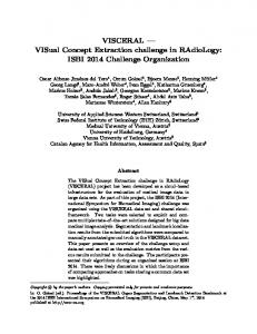
Player E

One Finger Two Fingers

Player O One Finger Two Fingers (2, −2) (−3, 3) (−3, 3) (4, −4)

Figure 1: Reward functions (RE , RO ) for two-finger Morra. and two reward functions Ra , Ro : A × O → R for a and o. It is zero-sum iff Ra = −Ro ; we then often omit Ro and abbreviate Ra by R. The behavior of the agents in a matrix game is expressed through the notions of pure and mixed strategies. Pure strategies specify a single action that an agent should execute, while mixed strategies specify a set of possible actions to be executed, where every action in this set is associated with the probability with which it should be executed. Formally, a pure (resp., mixed) strategy specifies which action an agent should execute (resp., which actions an agent should execute with which probability). If the agents a and o play the pure strategies a ∈ A and o ∈ O, respectively, then they receive the rewards Ra (a, o) and Ro (a, o), respectively. Let PD(A) (resp., PD(O)) denote the set of all probability functions over P PA (resp., O), that is, the set of all mappings µ from A (resp., O) to [0, 1] such that a∈A µ(a) = 1 (resp., o∈O µ(o) = 1). If the agents a and o play the mixed strategies µa ∈ PD(A) and µo ∈P PD(O), respectively, then the expected reward to agent k ∈ {a, o} is Rk (µa , µo ) = E[Rk (a, o)|µa , µo ] = a∈A, o∈O µa (a) · µo (o) · Rk (a, o). Towards optimal behavior of the agents in a matrix game, we are especially interested in pairs of mixed strategies (µa , µo ), called Nash equilibria, where no agent has the incentive to deviate from its half of the pair, once the other agent plays the other half: (µa , µo ) is a Nash equilibrium (or Nash pair) for G iff (i) Ra (µ0a , µo ) 6 Ra (µa , µo ) for any mixed µ0a , and (ii) Ro (µa , µ0o ) 6 Ro (µa , µo ) for any mixed µ0o . Every two-player matrix game G has at least one Nash pair among its mixed (but not necessarily pure) strategy pairs, and many have multiple Nash pairs. The Nash pairs can be computed by linear complementary programming and linear programming in the general and the zero-sum case, respectively. A Nash selection function f associates with each matrix game G a unique Nash equilibrium f (G) = (fa (G), fo (G)); the reward to k ∈ {a, o} under f (G) is then denoted by vfk (G). In the zero-sum case, if (µa , µo ) and (µ0a , µ0o ) are two Nash equilibria of G, then Ra (µa , µo ) = Ra (µ0a , 0 µo ), and also (µa , µ0o ) and (µ0a , µo ) are Nash equilibria of G. That is, the expected reward to the agents is the same under any Nash equilibrium, and Nash equilibria can be freely “mixed” to form new Nash equilibria. The strategies of agent a in Nash equilibria are the optimal solutions of the following linear program: max v subject to P µ(a) · Ra (a, o) > v for all o ∈ O, Pa∈A a∈A µ(a) = 1, and µ(a) > 0 for all a ∈ A. Furthermore, the expected reward to agent a under a Nash equilibrium is the optimal value of the above linear program. Example 10 (Two-Finger Morra) In the zero-sum matrix game two-finger Morra [35], two players E and O simultaneously show one or two fingers. Let f be the total number of fingers shown. If f is odd, then O gets f dollars from E, and if f is even, then E gets f dollars from O (see Fig. 1). A pure strategy

10


for player E (or O) is to show two fingers, while a mixed strategy for player E (or O) is to show one finger with the probability 7/12 and two fingers with the probability 5/12. The mixed strategy profile where each player shows one finger with the probability 7/12 and two fingers with the probability 5/12 is a Nash pair.

2.7

Stochastic Games

Stochastic games [29], or also called Markov games [39, 23], generalize both matrix games [41] and (fully observable) Markov decision processes (MDPs) [33]. A (two-player) stochastic game consists of a set of states S, a matrix game for every state s ∈ S (with common sets of actions for each agent), and a transition function that associates with every state s ∈ S and joint action of the agents a probability distribution on future states s0 ∈ S. Formally, a (two-player) stochastic game G = (S, A, O, P, Ra , Ro ) consists of a finite nonempty set of states S, two finite nonempty sets of actions A and O for two agents a and o, respectively, a transition function P : S × A × O → PD(S) (which associates with every triple (s, a, o) ∈ S × A × O a probability function P (s, a, o)( · ) over S, abbreviated as P ( · |s, a, o) or P ( · |s, (a, o))), and two reward functions Ra , Ro : S × A × O → R for a and o. It is zero-sum iff Ra = − Ro ; we then often omit Ro and abbreviate Ra by R. Assuming a finite horizon H > 0, a pure (resp., mixed) time-dependent policy associates with every state s ∈ S and number of steps to go h ∈ {0, . . . , H} a pure (resp., mixed) matrix-game strategy. A pure (resp., mixed) policy profile π = (πa , πo ) consists of a pure (resp., mixed) policy πk for each agent k ∈ {a, o}. The H-step value to agent k ∈ {a, o} under a start state s ∈ S and the pure policy profile π = (πa , πo ), denoted Gk (H, s, π), is defined by: ( Rk (s, π(s, H)) if H = 0; Gk (H, s, π) = P 0 0 Rk (s, π(s, H)) + s0 ∈S P (s |s, π(s, H)) · Gk (H−1, s , π) if H > 0. The expected H-step value to agent k ∈ {a, o} under a start state s and the mixed policy profile π = (πa , πo ), denoted Gk (H, s, π), is defined by: ( E[Rk (s, a) | π(s, H)] if H = 0; Gk (H, s, π) = P 0 0 E[Rk (s, a) + s0 ∈S P (s |s, a) · Gk (H−1, s , π) | π(s, H)] if H > 0. Finite-horizon Nash equilibria for stochastic games are then defined as follows. A mixed policy profile π = (πa , πo ) is a (H-step) Nash equilibrium (or (H-step) Nash pair) of G iff for every agent k ∈ {a, o} and every start state s ∈ S, it holds that Gk (H, s, π C πk0 ) 6 Gk (H, s, π) for every mixed policy πk0 , where π C πk0 is obtained from π by replacing πk by πk0 . Every stochastic game G has at least one Nash pair among its mixed (but not necessarily pure) policy profiles, and it may have exponentially many Nash pairs. Nash pairs for G can be computed by finite-horizon value iteration from local Nash pairs of matrix games as follows [20]. We assume an arbitrary Nash selection function f for matrix games G = (A, O, Ra , Ro ). For every state s ∈ S and every number of steps to go h ∈ {0, . . . , H}, the matrix game G[s, h] = (A, O, Qa [s, h], Qo [s, h]) is defined by: ( Rk (s, a) if h = 0; Qk [s, h](a) = P 0 i 0 Rk (s, a) + s0 ∈S P (s |s, a) · vf (G[s , h−1]) if h > 0, for every joint action a ∈ A =×i∈I Ai and every agent k ∈ {a, o}. For every agent k ∈ {a, o}, let the mixed policy πk be defined by πk (s, h) = fk (G[s, h]) for every s ∈ S and h ∈ {0, . . . , H}. Then, π = (πa , πo ) is


11

a H-step Nash pair of G, and it holds Gk (H, s, π) = vfk (G[s, H]) for every agent k ∈ {a, o} and every state s ∈ S. In the zero-sum case, by induction on h ∈ {0, . . . , H}, it is easy to see that, for every s ∈ S and h ∈ {0, . . . , H}, the normal form game G[s, h] is also zero-sum. Moreover, all Nash pairs that are computed by the above finite-horizon value iteration produce the same expected H-step value, and they can be freely “mixed” to form new Nash pairs.

2.8

Learning Optimal Policies

Q-learning [42, 43] is a reinforcement learning technique, which allows to solve an MDP without a model (that is, transition and reward functions) and can be used online. The value Q(s, a) is the expected discounted sum of future payoffs obtained by executing a from the state s and following an optimal policy. After being initialized to arbitrary numbers, the Q-values are estimated through the agent’s experience. For each execution of an action a leading from the state s to the (observed) state s0 , the agent receives a reward r (from the environment), and the Q-value update is Q(s, a) := (1 − α) · Q(s, a) + α · (r + γ · max Q(s0 , a0 )) , 0 a ∈A

where γ ∈ (0, 1) (resp., α ∈ [0, 1)) is the discount factor (resp., learning rate). This algorithm converges to the correct Q-values with probability 1 assuming that every action is executed in every state infinitely many times, and that α is decayed appropriately. Convergence also holds in the non-discounting case (γ = 1) in the presence of reward-free absorbing states, which are eventually reached from any non-absorbing state with positive probability. Littman [23] extends Q-learning to learning an optimal mixed policy in a zero-sum two-player stochastic game. Here, the Q-value update is Q(s, a, o) := (1 − α) · Q(s, a, o) + α · (r + γ · max min 0

µ∈PD(A) o ∈O

X

Q(s0 , a0 , o0 ) · µ(a0 )) ,

a0 ∈A

where the “maxmin”-term is the expected reward of a Nash pair for a zero-sum matrix game.

3

Adaptive GTGolog (AGTGolog)

In this section, we first define the domain theory behind the agent programming language Adaptive GTGolog (AGTGolog) and then the syntax of AGTGolog.

3.1

Domain Theory of AGTGolog

A domain theory DT = (AT , ST , OT ) of AGTGolog consists of a basic action theory AT , a stochastic theory ST , and an optimization theory OT , as defined below. We first give some preliminaries. We assume two zero-sum competing agents a and o (called agent and opponent, respectively, where the former is under our control, while the latter is not). The set of primitive actions is partitioned into the sets of primitive actions A and O of agents a and o, respectively. A two-agent action is any concurrent action c over A ∪ O such that |c ∩ A| 6 1 and |c ∩ O| 6 1. We often write a, o, and ako to abbreviate {a} ⊆ A, {o} ⊆ O, and {a, o} ⊆ A ∪ O, respectively.

12


Example 11 The concurrent actions {moveTo(a, 1, 2)} ⊆ A and {moveTo(o, 2, 3)} ⊆ O are single-agent actions of a and o, respectively, and thus also two-agent actions, while the concurrent action {moveTo(a, 1, 2), moveTo(o, 2, 3)} ⊆ A ∪ O is only a two-agent action, but not a single-agent action of a or o. A state formula over “~x, s” is a formula φ(~x, s) in which all predicate symbols are fluents, and the only free variables are the non-situation variables ~x and the situation variable s. A state partition over “~x, s” is a nonempty set of state formulas P (~x, s) = {φi (~x, s) | i ∈ {1, Wm. . . , m}} such that (i) ∀~x, s (φi (~x, s) ⇒ ¬φj (~x, s)) is valid for all i, j ∈ {1, . . . , m} with j > i, (ii) ∀~x, s ( i=1 φi (~x, s)) is valid, and (iii) every ∃~x, s (φi (~x, s)) is satisfiable. For state partitions P1 and P2 , we define their product by P1 ⊗ P2 = {ψ1 ∧ ψ2 | ψ1 ∈ P1 , ψ2 ∈ P2 , ψ1 ∧ ψ2 6= ⊥} . We often omit the arguments of a state formula when they are clear from the context. We next define the stochastic theory. As usual [36, 18, 2], every stochastic action a is expressed by a finite number of deterministic actions n1 , . . . , nk . When the stochastic action a is executed in the situation s, then “nature” chooses and executes with a certain probability exactly one of its deterministic actions ni with i ∈ {1, . . . , k}. Example 12 The stochastic action moveS (ag, x, y) of moving the agent ag to the position (x, y) in the situation s may have the effect that ag moves to (x, y) with the probability p and that ag moves to (x, y + 1) with the probability 1 − p, which is realized by making “nature” choose and execute exactly one of the two deterministic actions moveTo(ag, x, y) and moveTo(ag, x, y + 1) with the probabilities p and 1 − p, respectively. We use the predicate stochastic to connect the stochastic action a in the situation s to the deterministic actions n1 , . . . , nk , that is, stochastic(a, s, ni ) is true for all i ∈ {1, . . . , k}. We also specify a state partition a,n (~x, s) = {φa,n x, s) | j ∈ {1, . . . , m}} to group together situations s with common p such that “nature” Ppr j (~ chooses n in s with probability p, denoted prob(a(~x), n(~x), s) = p :2 V a,n ∃p1 , . . . , pm (p1 + · · · + pm = 1 ∧ m x, s) ⇔ prob(a(~x), n(~x), s) = pj )) . j=1 (φj (~ A stochastic action s is indirectly represented by providing a successor state axiom for each associated nature choice n; see also Example 14. Thus, AT is extended to a probabilistic setting in a minimal way. We assume that the domain is fully observable. For this reason, we introduce observability axioms, which disambiguate the state of the world after executing a stochastic action. This condition is represented by the predicate condStAct(c, s, n), where c is a stochastic action, s is a situation, n is a deterministic component of c, and condStAct(c, s, n) is true iff executing c in s has resulted in actually executing n. Similar axioms are introduced to observe which actions the two agents have chosen. Example 13 After executing c = moveS (ag, x, y) in the situation s, we test the predicates at(ag, x, y, do(c, s)) and at(ag, x, y + 1, do(c, s)) to check which of the two deterministic actions (that is, either moveTo(ag, x, y) or moveTo(ag, x, y + 1)) was actually executed. The predicate condStAct(c, s, n) for the stochastic action c = moveS (ag, x, y) is defined by: def

condStAct(c, s, {moveTo(ag, x, y)}) = at(ag, x, y, do(c, s)) , def

condStAct(c, s, {moveTo(ag, x, y+1)}) = at(ag, x, y+1, do(c, s)) . 2 Note that we specify only partitions of state formulas that group together situations with common transition probabilities, but not the transition probabilities themselves.


13

o2 o1 o3

a

o5

o ’s base

o4 o a ’s base Figure 2: Logistics Domain.

α (~ As for the optimization theory, for every two-agent action α, we specify a state partition Prw x, s) = α {φk (~x, s) | k ∈ {1, . . . , q}} to group together situations s with common r such that α(~x) and s assign the reward r to a, denoted reward (α(~x), s) = r :3

V ∃r1 , . . . , rq ( qk=1 (φαk (~x, s) ⇔ reward (α(~x), s) = rk )) .

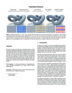
Example 14 (Logistics Domain cont’d) Consider the following scenario in a multi-agent logistics domain. We have an undirected graph of n locations connected by m edges (see Fig. 2). There are two agents, denoted a and o, which occupy one location each and move along the edges. The two agents can move one step to one of the directly connected locations, or remain stationary. Each agent can also pick up one object, and drop it at its base. Each action of the two agents can fail, resulting in a stationary move. Any carried object drops when the two agents collide. After each step, a and o receive (from the environment) the (zero-sum) rewards ra − ro and ro − ra , respectively, where rag , ag ∈ {a, o}, is −1, 2, and 10 when ag moves to a new location or remains stationary, ag picks up a new object, and ag brings an object to its base, respectively. The domain theory DT = (AT , ST , OT ) for the above logistics domain is defined as follows. As for the basic action theory AT , we assume the deterministic actions move(ag, x) (the agent ag moves to the location x), pickUp(ag, obj ) (the agent ag picks up the object obj ), drop(ag, obj ) (the agent ag drops the object obj ), and nop (no action), as well as the relational fluents at(q, x, s) (the agent or object q is at the location x in the situation s), onFloor (obj , x, s) (the object obj is on the floor at the location x in the situation s), and holds(ag, obj , s) (the agent ag holds the object obj in the situation s), which are defined 3 Note that we specify only partitions of state formulas that group together situations with common rewards, but not the rewards themselves.

14


through the following successor state axioms: at(ag, x, do(c, s)) ≡ at(ag, x, s) ∧ ¬∃y (move(ag, y) ∈ c) ∨ move(ag, x) ∈ c ; onFloor (obj , x, do(c, s)) ≡ (onFloor (obj , x, s) ∧ ¬∃ag (pickUp(ag, obj ) ∈ c) ∨ ∃ag ((drop(ag, obj ) ∈ c ∨ collision(c, s)) ∧ at(ag, x, s) ∧ holds(ag, obj , s))) ; holds(ag, obj , do(c, s)) ≡ holds(ag, obj , s) ∧ drop(ag, obj ) 6∈ c ∧ ¬collision(c, s) ∨ pickUp(ag, obj ) ∈ c . Here, collision(c, s) encodes that the concurrent action c causes a collision between the two agents a and o in the situation s : def

collision(c, s) = ∃x (move(a, x) ∈ c ∧ move(o, x) ∈ c) . The deterministic actions move(ag, x), pickUp(ag, obj ), drop(ag, obj ), and nop(ag) are associated with precondition axioms as follows: Poss(move(ag, x), s) ≡ ∃y (at(ag, y, s) ∧ connects(y, x)) ; Poss(pickUp(ag, obj ), s) ≡ ∃y (at(ag, y, s) ∧ onFloor (obj , y, s)) ∧ ¬∃x holds(ag, x, s) ; Poss(drop(ag, obj ), s) ≡ holds(ag, obj , s) ; Poss(nop(ag), s) ≡ > . Furthermore, we assume the following additional precondition axiom, which encodes that two agents cannot pick up the same object at the same time (where ag 6= ag 0 ): Poss({pickUp(ag, obj ), pickUp(ag 0 , obj 0 )}, s) ≡ ∃x, x0 (at(ag, x, s) ∧ at(ag 0 , x0 , s) ∧ x 6= x0 ∧ obj 6= obj 0 ) . As for the stochastic theory ST , we assume the stochastic actions moveS (ag, m) (the agent ag moves to one of the possible locations m), pickUpS (ag, obj ) (the agent ag picks up the object obj ), dropS (ag, obj ) a,n = {>} (the agent ag drops the object obj ), which may succeed or fail. We assume the state partition Ppr for each pair consisting of a stochastic action a and one of its deterministic components n: ∃p (p > 0 ∧ prob(moveS (ag, d), move(ag, d), s) = p ∧ prob(moveS (ag, d), nop(ag), s) = 1 − p) ; ∃p (p > 0 ∧ prob(pickUpS (ag, obj ), pickUp(ag, obj ), s) = p ∧ prob(pickUpS (ag, obj ), nop(ag), s) = 1 − p) ; ∃p (p > 0 ∧ prob(dropS (ag, obj ), drop(ag, obj ), s) = p ∧ prob(dropS (ag, obj ), nop(ag), s) = 1 − p) ; ∃p (prob(ako, a0 ko0 , s) = p ≡ ∃p1 , p2 (prob(a, a0 , s) = p1 ∧ prob(o, o0 , s) = p2 ∧ p = p1 · p2 )) . As for the optimization theory OT , we define the reward function reward as follows: reward (a, s) = r ≡ ∃ra , ro (rewAg(a, a, s) = ra ∧ rewAg(o, a, s) = ro ∧ r = ra − ro ) ; V ag,a ∃r1 , . . . , rm ( m (s) ⇔ rewAg(ag, a, s) = rj )) . j=1 (φj ag,a Here, the state partitions Prw (s) = {φag,a (s) | j ∈ {1, . . . , m}} for the agent ag and the different actions j a ∈ {moveS (ag, x), pickUpS (ag, obj ), dropS (ag, obj )} are as follows:


15

ag,a • If a = moveS (ag, x), then Prw (s) = {>}. Informally, for each context, a moving action does not affect the immediate reward. Hence, we do not distinguish between different states, and we get the trivial partition defined by the true formula. ag,a • If a = pickUpS (ag, obj ), then Prw (s) = {¬h∧ato, ¬h∧¬ato, h}, where h = ∃x(holds(ag, x, s)) (the agent ag holds an object) and ato = ∃y, obj (at(ag, y, s) ∧ on- Floor (obj , y, s)) (the agent ag is close to an object). Informally, the immediate reward depends on whether

– ag holds no object but is close to an object (¬h ∧ ato), – ag holds no object and is also far from an object (¬h ∧ ¬ato), or – ag holds an object (h). ag,a • If a = dropS (ag, obj ), then Prw (s) = {h ∧ atb, h ∧ ¬atb, ¬h}, where h is as above and atb = atBase(ag, s) = ∃y (at(ag, y, s) ∧ base(ag, y)) (the agent ag is at its base). Informally, the immediate reward depends on whether

– ag holds an object and is at its base (h ∧ atb), – ag holds an object and is not at its base (h ∧ ¬atb), or – ag holds no object (¬h).

3.2

Syntax of AGTGolog

In the sequel, let DT be a domain theory. AGTGolog has the same syntax as standard GTGolog, which is defined by induction as follows. A program p in AGTGolog has one of the following forms (where α is a two-agent action or the empty action nop (which is always executable and does not change the state of the world), φ is a condition, p, p1 , p2 are programs without procedure declarations, P1 , . . . , Pn are procedure names, x, ~x1 , . . . , ~xn are arguments, and a1 , . . . , an and o1 , . . . , om are actions of agents a and o, respectively, and τ = {τ1 , τ2 , . . . , τn } is a finite nonempty set of ground terms): 1. Deterministic or stochastic action: α. Do α. 2. Nondeterministic action choice of agent a: choice(a : a1 | · · · |an ). Do an optimal action (for agent a) among a1 , . . . , an . 3. Nondeterministic action choice of agent o: choice(o : o1 | · · · |om ). Do an optimal action (for agent o) among o1 , . . . , om . 4. Nondeterministic joint action choice: choice(a : a1 |· · ·|an ) k choice(o : o1 |· · ·|om ). Do every action ai koj with an optimal probability µa (ai ) · µo (oj ). 5. Test action: φ?. Test the truth of φ in the current situation. 6. Sequence: [p1 ; p2 ]. Do p1 followed by p2 . 7. Nondeterministic choice of two programs: (p1 | p2 ). Do an optimal program among p1 and p2 .

16


8. Nondeterministic choice of program argument: π[x : τ ](p(x)). Do an optimal program p(x) with x ∈ τ . 9. Nondeterministic iteration: p? . Do p optimally zero or more times. 10. Conditional: if φ then p1 else p2 . If φ is true in the current situation, then do p1 else do p2 . 11. While-loop: while φ do p. While φ is true in the current situation, do p. 12. Procedures: proc P1 (~x1 ) p1 end ; . . .; proc Pn (~xn ) pn end ; p. The procedures named P1 , . . . , Pn , respectively, are declared and can be used in p. Hence, compared to Golog, we now also have two-agent actions (instead of only primitive or concurrent actions) and stochastic actions (instead of only deterministic actions). Moreover, we now additionally have three different kinds of nondeterministic action choices for the two agents in (2)–(4), where one or both of the two agents can choose among a finite set of single-agent actions. The two-agent actions and the choice operators in (3) and (4) are also new compared to DTGolog. The formal semantics of (2)–(4) is defined in such a way that an optimal action is chosen for each of the two agents. Similarly, an optimal program is chosen in (7)–(9). If there are several optimal action or program choices, then we additionally assume a total order on these choices and take the preferred choice according to this order (for example, choose the leftmost optimal action in (2)–(4) and the leftmost optimal program in (7)). As usual, the sequence operator “;” is associative (for example, [[p1 ; p2 ]; p3 ] and [p1 ; [p2 ; p3 ]] mean the same), and “p1 ; p2 ”, “if φ then p1 ”, and “πx (p(x))” often abbreviate “[p1 ; p2 ]”, “if φ then p1 else nop”, and π[x : τ ](p(x)), respectively, when there is no danger of confusion. Example 15 (Logistics Domain cont’d) We define some AGTGolog programs relative to the domain theory DT = (AT , ST , OT ) of Example 14. The main task of the agent a (and the opponent o) is to take one object and drop it at the base. This can be described by the following AGTGolog procedure: proc task (a, o) getObject(a, o) ; carryToBase(a, o) end. Here, getObject(a, o) is an AGTGolog procedure for searching and picking up an object, while carryToBase(a, o) describes a partially specified behavior where the agent a (competing with o) is trying to move to its base in order to drop an object: proc getObject(a, o) π[y : loc](π[x : obj ](moveS (a, y) ; ?(onFloor (x, y)) ; pickProc(a, o, x))) end. proc carryToBase(a, o) π[y : loc](moveS (a, y) ; if atBase(a) then π[x : obj ](dropS (a, x)) else carryToBase(a, o)) end.


17

Here, loc (resp., obj ) is the set of possible locations (resp., objects). The subsequent procedure pickProc(a, o, x) encodes that if the two agents a and o are at the same location, then they have to compete in order to pick up an object, otherwise the agent a can directly use the primitive action pickUpS (a, x): proc pickProc(a, o, x) if atSameLocation(a, o) then tryToPickUp(a, o, x) else pickUpS (a, x) end. Here, the joint choices of the two agents a and o when they are at the same location are specified by the following procedure tryToPickUp(a, o, x) (which will be instantiated by a mixed policy): proc tryToPickUp(a, o, x) choice(a : pickUpS (a, x) | nop(a)) k choice(o : pickUpS (o, x) | nop(o)) end. Note that in the case of a concurrent attempt of picking up the same object, by the concurrent precondition axiom, at least one of the two agents is forced to fail.

4

State Partition Generation

In this section, we define joint state partitions for AGTGolog programs relative to finite horizons. Informally, during the learning of action rewards and transition probabilities for an AGTGolog program p, we randomly choose an initial state of the environment and start the execution of the program p, during which we receive action rewards and make nature choose the outcome of probabilistic transitions. Hence, the initially chosen state of the environment should fix in advance appropriate elements of the state partitions for the action rewards and the transition probabilities. Furthermore, whenever the program p arrives at a point with several action or program alternatives, the initially chosen state of the environment should allow for choosing any of these alternatives. That is, we have to construct a joint state partition from all state partitions of action rewards and transition probabilities, considering also all action and program alternatives, in the program p within a finite horizon. More formally, a machine state (p, h) consists of an AGTGolog program p and a horizon h > 0. A machine state (p, h) precedes another machine state (p0 , h0 ), denoted (p, h) B (p0 , h0 ), iff p0 is a possible remaining of p after running p for h − h0 steps. A joint state (φ, p, h) consists of a state formula φ and a machine state (p, h). Informally, a machine state represents the executive state of the agent, while a joint state represents both the state of the environment and the executive state of the agent. Every machine state (p, h) is now associated with a state partition, denoted SF (p, h) = {φ1 (~x, s), . . . , φm (~x, s)}, which is defined by induction on the structure of AGTGolog programs as follows: 1. Null program or zero horizon: SF (nil , h) = SF (p, 0) = {>} . At the program or horizon end, the state partition is given by {>}. Indeed, when the program or the horizon ends, then no more choices are needed, and therefore we have a unique context representing the end of the program.

18


2. Deterministic first program action: a (~ SF (a; p0 , h) = ((Prw x, s) ⊗ {Regr (φ(~x, do(a, s)) ∧ Poss(a, s) | φ(~x, s) ∈ SF (p0 , h − 1)}) ∪ {¬Poss(a, s)}) \ {⊥} .

Here, the state partition for a; p0 with horizon h is obtained as the product of the reward partition a (~ Prw x, s), the state partition SF (p0 , h − 1) of the next machine state (p0 , h − 1), and the executability partition {¬Poss(a, s), Poss(a, s)}. 3. Stochastic first program action (nature choice): Nk a,ni 0 SF (a; p0 , h) = x, s)), i=1 (SF (ni ; p , h) ⊗ Ppr (~ where n1 , . . . , nk are the deterministic components of a. That is, the partition for a; p0 in h, where a is stochastic, is the product of the state partitions SF (ni ; p0, h) relative to the deterministic components a,ni ni of a combined with the partitions Ppr . 4. Nondeterministic first program action (choice of agent k): Nn 0 SF (choice(k : a1 | · · · |an ); p0 , h) = i=1 SF (ai ; p , h) , where a1 , . . . , an are two-agent actions. That is, the state partition for a single choice of actions is the product of the state partitions for the possible choices. 5. Nondeterministic joint action choice: SF (choice(a : a1 | · · · |an ) k Nn,m 0 choice(o : o1 | · · · |om ); p0 , h) = i=1,j=1 SF (ai koj ; p , h) , where a1 , . . . , an and o1 , . . . , om are the possible choices for a and o respectively. The associated state partition is obtained from the partitions generated by the possible concurrent executions ai koj . 6. Test action: SF (φ?; p0 , h) = ({φ} ⊗ SF (p0 , h)) ∪ {¬φ} . The partition for (φ?; p0 , h) is obtained by composing the partition {φ, ¬φ} induced by the test φ? with the state partition for (p0 , h). 7. Nondeterministic choice of two programs: SF ((p1 | p2 ); p0 , h) = SF (p1 ; p0 , h) ⊗ SF (p2 ; p0 , h) . The state partition for a nondeterministic choice of two programs is obtained as the product of the state partitions associated with the possible programs. 8. Nondeterministic choice of program argument: SF (π[x : {τ1 , . . . , τn }](p(x)); p0 , h) = {φ1 (τ1 ) ∧ · · · ∧ φn (τn ) | φ1 (x), . . . , φn (x) ∈ SF (p(x : {τ1 , . . . , τn }); p0 , h)} \ {⊥} . The state partition for a nondeterministic choice of program argument is obtained as the product of the state partitions associated with the possible program instantiations. Here, SF (p(x : {τ1 , . . . , τn }); p0 , h) denotes a state partition that is parameterized via the variable x, which may take on any value from {τ1 , . . . , τn }.


19

9. Nondeterministic iteration: SF (p? ; p0 , h) = SF (p; p? ; p0 , h) ⊗ SF (p0 , h) . This case is reduced to procedures and nondeterministic choice of two programs. 10. Conditional: SF (if ψ then p1 else p2 ; p0 , h) = ({ψ} ⊗ SF (p1 ; p0 , h)) ∪ ({¬ψ} ⊗ SF (p2 ; p0 , h)) . The state partition for “if ψ then p1 else p2 ; p0 , h” is obtained by composing the partition {ψ, ¬ψ} with the state partitions for “p1 ; p0 , h” and “p2 ; p0 , h”. 11. While-loop: SF (while ψ do p; p0 , h) = ({ψ} ⊗ SF (p; while ψ do p; p0 , h)) ∪ ({¬ψ} ⊗ SF (p0 , h)) . The state partition for “while ψ do p; p0 , h” is obtained by composing the partition {ψ, ¬ψ} with the state partitions for “p; while ψ do p; p0 , h” and “p0 , h”. 12. Procedures: SF (proc P1 (~x1 ) p1 end ; . . . ; proc Pn (~xn ) pn end ; p, h) = SF (phproc P1 (~x1 ) p1 end ; . . . ; proc Pn (~xn ) pn endi; p0 , h) ; SF (Pi (~xi ); p0 hdi, h) = SF (pd (Pi (~xi )); p0 , h) . We consider the cases of (1) handling procedure declarations and (2) handling procedure calls. To this end, we slightly extend the first argument of SF by a store for procedure declarations, which can be safely ignored in all the other above cases. Here, pd (Pi (~xi )) denotes the code from d for the procedure call Pi (~xi ). Example 16 (Logistics Domain cont’d) Some joint states are (φ1 , p, h) and (φ2 , p, h), where (p, h) is the machine state consisting of the AGTGolog program move(a, x) k move(o, y) ; nil and the horizon h = 1, and φ1 and φ2 are given as follows: φ1

=

∃k (onFloor (k, x, s)) ∧ ∃l (onFloor (l, y, s)) ∧ ∃z (at(a, z, s) ∧ connects(z, x)) ∧ ∃w (at(o, w, s) ∧ connects(w, y)) ;

φ2

=

¬∃k (onFloor (k, x, s)) ∧ ∃l (onFloor (l, y, s)) ∧ ∃z (at(a, z, s) ∧ connects(z, x)) ∧ ∃w (at(o, w, s) ∧ connects(w, y)) .

As for the worst-case number of state formulas in the generated state partitions, it is not difficult to h verify that the worst-case cardinality of SF (p, h) is in O((m n)a ), where (i) n is the maximal number of state formulas in the input probability and the input reward partitions; (ii) a is the maximum among (ii.a) the maximal number of actions of an agent in nondeterministic (single or joint) action choices in p, (ii.b) the maximal number of choices of nature after stochastic actions in p, and (ii.c) the nondeterministic branching

20


factor of p, which is the maximal number of alternative program choices (via nondeterministic choices of two programs, nondeterministic choices of program arguments, and nondeterministic iterations) at any step within h; and (iii) m is the conditional branching factor of p, which is the maximal number of branchings via conditionals and while-loops of p at any step within h. Although this worst-case number seems to be quite large, observe that many of the generated state formulas will be the false formula, especially when the input state partitions are logically very similar. Furthermore, an upper bound for the number of state formulas in state partitions is also the size of the state space. Finally, in many applications in practice, one can assume that the horizon is very small and bounded by a constant, and that it is not necessary to explore the whole state space in the learning algorithm.

5

Learning Optimal Policies

We now show how to learn optimal policies for AGTGolog programs relative to finite horizons. Intuitively, given an AGTGolog program p and a horizon h > 0, an h-step policy π for p relative to a domain theory DT is obtained from the h-horizon part of p by replacing every single-agent choice by a single action, and every multi-agent choice by a collection of probability distributions, one over the actions of each agent. Note that the learning algorithm also implicitly learns the transition probabilities and rewards. Note also that the convergence and optimality of the learning algorithm is proved in Section 7. We first describe the overall learning algorithm. We then define selection functions and describe the updating step of the learning algorithm. We finally sketch how success probabilities / flags can be added and describe a (very) preliminary implementation.

5.1

Learning Algorithm

The main learning algorithm is Learn in Algorithm 1. The algorithm takes as input an AGTGolog program p and a finite horizon h > 0 (note that h is the maximal number of steps to go, that is, the maximal number of actions to be executed). It generates as output an optimal h0 -step policy π(σ) along with its expected utility v(σ), for each joint state σ = (φ, p0 , h0 ) such that φ ∈ SF (p0 , h0 ) and (p, h) B (p0 , h0 ). We use a hierarchical version of Q-learning. In line 1, we initialize the learning rate α to 1, which decays at each learning cycle according to decay. In lines 2 and 3, we also initialize to 0 the variables v(σ) representing the current expected utilities. At each cycle, the current state φ ∈ SF (p, h) is evaluated (that is, the agent evaluates which of the state formulas describes the current state of the world). Then, from the joint state σ = (φ, p, h), the procedure Update(φ, p, h) (see Section 5.3) executes the program p with horizon h, and updates and refines the expected utilities v(σ) and the policies π(σ). At the end of the execution of Update, if the learning rate is greater than a suitable threshold ε, then the current state φ is evaluated, and a new learning cycle starts. At the end of the algorithm Learn, for suitable decay and ε, each possible execution of (p, h) from each φ is performed often enough to obtain convergence. That is, the agent executes the program (p, h) several times refining its pairs of expected utilities v(σ) and its policies π(σ) until they do not change anymore.

5.2

Selection Functions

In the updating step, we use selection functions for minimal arguments in minimizations, maximal arguments in maximizations, and Nash equilibria of zero-sum matrix games of the form G = (I, (Ai )i∈I , R),


21

Algorithm 1 Learn(p, h) Require: AGTGolog program p and a finite horizon h > 0. Ensure: optimal h0 -step policy π(σ) and its expected utility v(σ), for each σ = (φ, p0 , h0 ) such that φ ∈ SF (p0 , h0 ) and (p, h) B (p0 , h0 ). 1: α := 1; 2: for each σ = (φ, p0 , h0 ) such that φ ∈ SF (p0 , h0 ) and (p, h) B (p0 , h0 ) 3: do v(σ) := 0; 4: repeat 5: estimate φ ∈ SF (p, h); 6: Update(φ, p, h); 7: α := α · decay 8: until α < ε; 9: return (v(φ, p0 , h0 ), π(φ, p0 , h0 ))φ∈SF (p0 ,h0 ), (p,h)B(p0 ,h0 ) .

where I = {a, o} and Aa = {a1 , . . . , am } (resp., Ao = {o1 , . . . , on }) is a nonempty set of single-agent actions of agent a (resp., o). As for selecting minimal (resp., maximal) arguments in minimizations (resp., maximizations), we define prefArgmin(r1 , . . . , rn ) (resp., prefArgmax (r1 , . . . , rn )), where n > 1, as the unique index l ∈ {1, . . . , n} such that (i) rl is a minimal (resp., maximal) element among r1 , . . . , rn and (ii) the index l is minimal with (i). Intuitively, arguments with lower index are preferred to arguments with higher index. But we use slightly modified versions of these functions, which additionally take into account numerical imprecision due to convergence with probability 1: We define ε-prefArgmin(r1 , . . . , rn ) (resp., ε-prefArgmax (r1 , . . . , rn )), where n > 1 and ε > 0, as the unique index l ∈ {1, . . . , n} such that (i) rl is within the ε-range of a minimal (resp., maximal) element among r1 , . . . , rn and (ii) the index l is minimal with (i). These ε-variants of prefArgmin and prefArgmax then allow for pushing through the convergence with probability 1 of policies (see also Proposition 19). As for selecting Nash pairs of zero-sum matrix games G = (I, (Ai )i∈I , R), where I = {a, o} and Aa = {a1 , . . . , am } (resp., Ao = {o1 , . . . , on }) as above, the Nash selection function prefNash selects the pref Nash pair µpref = (µpref a , µo ) of G such that for every other Nash pair µ = (µa , µo ) of G there exist some k ∈ {1, . . . , m} and l ∈ {1, . . . , n} such that: • µpref a (ai ) = µa (ai ) for all i ∈ {1, . . . , k − 1}, • µpref a (ak ) > µa (ak ), • µpref o (oj ) = µo (oj ) for all j ∈ {1, . . . , l − 1}, and • µpref o (ol ) > µo (ol ). Intuitively, actions with lower index are given a higher probability than arguments with higher index. We compute prefNash(G) by linear programming. More concretely, let v be the expected reward to agent a unpref der a Nash pair of G. Then, prefNash(G) is the pair of mixed strategies µpref = (µpref a , µo ) ∈ PD(Aa ) × PD(Ao ) such that: • µpref a (ai ), for every i ∈ {1, . . . , m}, is the maximum of µa (ai ) subject to

22

INFSYS RR 1843-08-07 Pm

i=1 µa (ai )

· R(ai , oj ) > v for all j ∈ {1, . . . , n},

Pm

i=1 µa (ai ) = 1,

µa (ai ) > 0 for all i ∈ {1, . . . , m}, and µa (al ) = µpref a (al ) for every l ∈ {1, . . . , i − 1}; • µpref o (oj ), for every j ∈ {1, . . . , n}, is the maximum of µo (oj ) subject to Pn

j=1 µo (oj )

· R(ai , oj ) 6 v for all i ∈ {1, . . . , m},

Pn

j=1 µo (oj ) = 1,

µo (oj ) > 0 for all j ∈ {1, . . . , n}, and µo (ol ) = µpref o (ol ) for every l ∈ {1, . . . , j − 1}. To additionally take into account numerical imprecision due to convergence with probability 1, as in the case of prefArgmin and prefArgmax , we also use an ε-variant of prefNash, denoted ε-prefNash, where ε > 0, which is defined by ε-prefNash(G) = prefNash(G0 ), where the matrix game G0 is obtained from G be replacing any collection of rewards that lie within an ε-range of each other by their additive average. This ε-variant of prefNash allows for pushing through the convergence with probability 1 of policies (see also Proposition 20).

5.3

Updating Step

The procedure Update(φ, p, h) in Algorithms 2 and 3 implements the execution and update step of a Qlearning algorithm. Each joint state σ of the program p within the horizon h is associated with a variable v(σ), which store the current expected utility at σ, and a variable π(σ), which stores the current optimal policy at σ. The procedure Update(φ, p, h) updates these variables during an execution of the program p within the horizon h from a state φ ∈ SF (p, h). It is recursive, following the structure of the program. Algorithm 2 shows the first part of the procedure Update(φ, p, h). Lines 1–4 encode the basis of the induction: if the program is empty or the horizon is zero, then we set the expected utility and the policy to 0 and nil , respectively. In lines 5–8, we consider the non-executable cases: if a primitive action a is not executable in the current state formula (here, ¬Poss(a, φ) abbreviates DT ∪ φ |= ¬Poss(a, s)) or a test fails in the current state formula (here, ¬ψ[φ] stands for DT ∪ φ |= ¬ψ(s)), then we set the expected utility and the policy to 0 and stop (which stops the execution), respectively. In lines 9–14, we consider deterministic actions a (here, Poss(a, φ) is a shortcut for DT ∪ φ |= Poss(a, s)): after executing a, the agent receives the reward reward from the environment. Then, after executing the rest of the program from the next state formula (that is, do(a, φ), which is the state formula φ0 ∈ SF (p0 , h−1) such that Regr (φ0 (do(a, s))) = φ(s) relative to DT ) via Update(do(a, φ), p0 , h−1), the variables v(σ) and π(σ) for σ = (φ, a; p0 , h) are updated by adding the received reward to the current expected utility of the next joint state and adding a to the current policy of the next joint state, respectively. In lines 15–21, we consider stochastic actions a: after executing the stochastic action a, we observe the deterministic component nq chosen by “nature”, and we update the expected utilities similarly as in Q-learning, where the current utility is obtained as the sum of the old utility with factor 1 − α and of the updated utility (for the executed component) with factor α. The generated policy is a conditional plan where each possible execution is considered. Here, φi are the conditions to discriminate


23

Algorithm 2 Update(φ, p, h) Require: state formula φ, AGTGolog program p, and finite horizon h > 0. Ensure: updates v(σ) and π(σ), where σ = (φ, p, h). 1: if p = nil ∨ h = 0 then 2: v(σ) := 0; 3: π(σ) := nil 4: end if; 5: if p = a; p0 ∧¬Poss(a, φ) ∨ p = ψ?; p0 ∧¬ψ[φ] then 6: v(σ) := 0; 7: π(σ) := stop 8: end if; 9: if p = a; p0 ∧ Poss(a, φ) and a is deterministic then 10: execute a and observe reward ; 11: Update(do(a, φ), p0 , h−1); 12: v(σ) := v(do(a, φ), p0 , h−1) + reward ; 13: π(σ) := a; π(do(a, φ), p0 , h−1) 14: end if; 15: if p = a; p0 ∧ Poss(a, φ) and a is stochastic then 16: “nature” selects any deterministic action nq of the action a; 17: Update(φ, nq ; p0 , h); 18: v(σ) := (1 − α) · v(σ) + α · v(φ, nq ; p0 , h); 19: π(σ) := a; if φ1 then π(φ, n1 ; p0 , h) . . . 20: else if φk then π(φ, nk ; p0 , h) 21: end if; 22: if p = choice(a : a1 | · · · |an ); p0 then 23: select any q ∈ {1, . . . , n} with strategy explore (see below); 24: Update(φ, a:aq ; p0 , h); 25: v(σ) := maxi∈{1,...,n} v(φ, a:ai ; p0 , h); 26: k := ε-prefArgmax i∈{1,...,n} v(φ, a:ai ; p0 , h); 27: π(σ) := a:ak ; if φ1 then π(do(a:a1 , φ), p0 , h − 1) . . . 28: else if φn then π(do(a:an , φ), p0 , h − 1) 29: end if; 30: if p = choice(o : o1 | · · · |om ); p0 then 31: select any q ∈ {1, . . . , m} with strategy explore (see below); 32: Update(φ, o:oq ; p0 , h); 33: v(σ) := mini∈{1,...,m} v(φ, o:oi ; p0 , h); 34: k := ε-prefArgmin i∈{1,...,m} v(φ, o:oi ; p0 , h); 35: π(σ) := o:ok ; if φ1 then π(do(o:o1 , φ), p0 , h − 1) . . . 36: else if φm then π(do(o:om , φ), p0 , h − 1) 37: end if; 38: if p = choice(a : a1 | · · · |an ) k choice(o : o1 | · · · |om ); p0 then 39: select any r ∈ {1, . . . , n} and s ∈ {1, . . . , m} with strategy explore (see below); 40: Update(φ, a:ar ko:os ; p0 , h); 41: v(σ) := expected reward under a Nash pair of {ri,j = v(φ, a:ai ko:oj ; p0 , h) | i, j}; 42: (µa , µo ) := ε-prefNash({ri,j = v(φ, a:ai ko:oj ; p0 , h) | i, j}); 43: π(σ) := µa kµo ; if φ1 ∧ψ1 then π(do(a:a1 ko:o1 , φ), p0 , h − 1) . . . 44: else if φn ∧ψm then π(do(a:an ko:om , φ), p0 , h − 1) 45: end if; 46: . Update(φ, p, h) is continued in Algorithm 3.

24


Algorithm 3 Update(φ, p, h) (cont’d) 47: if p = ψ?; p0 ∧ (φ = ψ ∧ φ0 ) then 48: Update(φ0 , p0 , h); 49: v(σ) := v(φ0 , p0 , h); 50: π(σ) := π(φ0 , p0 , h) 51: end if; 52: if p = (p1 | p2 ); p0 then 53: select any i ∈ {1, 2} with strategy explore (see below); 54: Update(φ, pi ; p0 , h); 55: v(σ) := maxi∈{1,2} v(φ, pi ; p0 , h); 56: k := ε-prefArgmax i∈{1,2} v(φ, pi ; p0 , h); 57: π(σ) := π(φ, pk ; p0 , h) 58: end if; 59: if p = π[x : {τ1 , . . . , τn }](p(x)); p0 then 60: select any i ∈ {1, . . . , n} with strategy explore (see below); 61: v(σ) := maxi∈{1,...,n} v(φ, p(τi ); p0 , h); 62: k := ε-prefArgmax i∈{1,...,n} v(φ, p(τi ); p0 , h); 63: π(σ) := π(φ, p(τk ); p0 , h) 64: end if; 65: if p = p? ; p0 then 66: select any p1 = p; p? ; p0 or p2 = p0 with strategy explore (see below); 67: Update(φ, pi , h); 68: v(σ) := maxi∈{1,2} v(φ, pi , h); 69: k := ε-prefArgmax i∈{1,2} v(φ, pi , h); 70: π(σ) := π(φ, pk , h) 71: end if; 72: if p = “ if ψ then p1 else p2 ; p0 ” ∧ ((φ = ψ ∧ φ0 ) ∨ (φ = ¬ψ ∧ φ0 )) then 73: if φ = ψ ∧ φ0 then Update(φ0 , p1 ; p0 , h) else Update(φ0 , p2 ; p0 , h) 74: end if; 75: if p = “ while ψ do p; p0 ” ∧ ((φ = ψ ∧ φ0 ) ∨ (φ = ¬ψ ∧ φ0 )) then 76: if φ = ψ ∧ φ0 then Update(φ0 , p; while ψ do p; p0 , h) else Update(φ0 , p0 , h) 77: end if; 78: if p = “ proc P1 (~ x1 ) p1 end ; . . . ; proc Pn (~xn ) pn end ; p ” then 79: decl := “ proc P1 (~x1 ) p1 end ; . . . ; proc Pn (~xn ) pn end ”; 80: Update(φ, p, h) 81: end if; 82: if p = Pi (~ xi ); p0 then 83: extract the code pdecl (Pi (~xi )) for the procedure call Pi (~xi ) from decl ; 84: Update(φ, pdecl (Pi (~xi )); p0 , h) 85: end if.


25

the executed component (represented by the observability axioms). In lines 22–37, the code deals with the agent (resp., opponent) choice construct, and encodes how the agent learns an optimal action from the possible ones. Here, we first select one possible action according to an exploration strategy explore: with some probability p ∈ (0, 1), the agent (resp., opponent) selects randomly, and with the probability 1 − p, the agent (resp., opponent) selects an action according to the current optimal policy π(σ). That is, explore controls how often the agent (resp., opponent) deviates from the current optimal policy, ensuring a suitable exploration of the state space. After executing the selected action via Update, the expected utility v(σ) is updated with the utilities of a maximal (resp., minimal) choice, and π(σ) is updated with a conditional plan starting with this maximal (resp., minimal) choice. In lines 38–45, we consider the joint action choice of both agents. We select one action from the possible ones for each agent, using the strategy explore, similarly as described above. After executing the procedure Update along the selected joint action, v(σ) is updated with the expected reward under the pair of mixed strategies µa kµo specified by ε-prefNash from the matrix game of the possible joint actions (that is, the current expected utilities of the possible joint actions). Furthermore, π(σ) is updated with a conditional plan where each possible execution is considered. Here, φi and ψj are the conditions to discriminate the executed component for the agent and the opponent, respectively. Algorithm 3 shows the second part of the procedure Update(φ, p, h). Lines 47–51 define the successful test execution, that is, if DT ∪ φ |= ψ(s), then after executing the rest of the program (p0 , h), we update the expected utility and the policy with the ones for the program (p0 , h) from φ0 . Lines 52–58 encode the choice among two programs: one of the two programs is selected with exploration strategy explore, similarly as described above. After executing the selected program through Update, the variables v(σ) and π(σ) are updated considering the maximal among the utilities of the two programs. Finally, in lines 59–82, we essentially reduce all the remaining constructs to the previous ones.

5.4

Adding Success Probabilities / Flags

To extend the semantics and the learning algorithm of AGTGolog to also account for success probabilities / flags as in DTGolog, expected utilities u = hv, pr i consisting of an expected value v and a success probability pr ∈ [0, 1] are represented by the value f (u) = v (resp., f (u) = v + M ) iff pr = 0 (resp., pr > 0), where M is a sufficiently large number (which is greater than any possible expected value v). It is then not difficult to verify that u1 ≺ u2 iff f (u1 ) < f (u2 ) for all possible utilities u1 and u2 . To correctly compute such expected utilities in AGTGolog, one then has to slightly adapt some computations of expected utilities in the learning algorithm (in a similar way as in the GTGolog interpreter; see [11]).

5.5

Implementation

We have a (very) preliminary implementation, where the state formula generator is implemented in Eclipse Prolog, and the learning algorithm is realized in Eclipse Prolog embedded in C++, using the gltk library for linear programming (for the Nash solver). The learning algorithm uses the Eclipse engine for state formula evaluation and utility/policy update.

6

Example

We now illustrate the overall system working in the Logistics Domain.

26


Machine States (p, 3) (p1 , 3) (p01 , 3) (pi,j , 3) (p2 , 2) (p(y), 2) (p3 , 1)

State Partitions SF (p, 3) = ({asl } ⊗ SF (p1 , 3)) ∪ ({¬asl } ⊗ SF (p01 , 3)) N SF (p1 , 3) = i,j∈{1,2} SF (pi,j , 3) a (~ SF (p01 , 3) = (Prw x, s) ⊗ . . . SF (pi,j , 3) = . . . N SF (p2 , 2) = q∈loc SF (pq , 2) SF (p(y), 2) = ({atb y } ⊗ SF (p3 , 1)) ∪ ({¬atb y } ⊗ SF (p03 , 1)) SF (p3 , 1) = . . .

Figure 3: Machine states and state partitions for the program p = pickProc(a, o, x); carryToBase(a, o) and the horizon h = 3.

Example 17 (Logistics Domain cont’d) Consider again the domain theory DT = (AT , ST , OT ) for the Logistics Domain of Example 14 and the AGTGolog procedures of Example 15. Let the AGTGolog program p be given by p = pickProc(a, o, x); carryToBase(a, o) , and assume the horizon h = 3. Recall that a policy for p within h is obtained from p by replacing every single-agent choice in p within h by a single action, and every multi-agent choice in p within h by a collection of probability distributions, one over the actions of each agent. Learning an optimal policy now works as follows. First, we generate the state partition SF (p0 , h0 ) for every machine state (p0 , h0 ) of p within h, that is, for every machine state (p0 , h0 ) such that (p, h) B (p0 , h0 ). Then, we use Algorithm Learn for p and h to learn an optimal policy π(σ) for each joint state σ = (φ, p0 , h0 ) such that φ ∈ SF (p0 , h0 ) and (p, h) B (p0 , h0 ): we run several times p within h for φ ∈ SF (p, h) until the expected utility v and the policy π stabilize for each joint state σ = (φ, p0 , h0 , ) such that φ ∈ SF (p0 , h0 ) and (p, h) B (p0 , h0 ). Machine States. Given the program p, we consider the following machine states: (p, (p1 , (pi,j , (p01 , (p2 , (p(y), (p3 ,

3) 3) 3) 3) 2) 2) 1)

with with with with with with with

p = pickProc(a, o, x); carryToBase(a, o) , p1 = tryToPickUp(a, o, x); carryToBase(a, o) , pi,j = ai koj ; carryToBase(a, o) , p01 = pickUpS (a, x); carryToBase(a, o) , p2 = carryToBase(a, o) , p(y) = moveS (a, y); if atBase(a) then p3 else p2 , p3 = π[x : obj]dropS (a, x) .

These are in the following relations: (p, 3) B (p1 , 3) B (pi,j , 3) B (p2 , 2) B (pq , 2) B (p3 , 1) , (p, 3) B (p01 , 3) B (p2 , 2) B (pq , 2) B (p3 , 1) .

State Partitions and Policies. We now consider the state partitions and policies associated with the above machine states.


27

• (p, 3): The state partition for the machine state (p, 3) is given as follows: SF (p, 3) = ({asl } ⊗ SF (p1 , 3)) ∪ ({¬asl } ⊗ SF (p01 , 3)) , with asl = atSameLocation(a, o). In the learning algorithm, we then associate with every joint state (φ, p, 3), where φ = asl ∧φ0 ∈ SF (p, 3) (resp., φ = ¬asl ∧φ0 ∈ SF (p, 3)), the policy π(φ0 , p1 , 3) (resp., π(φ0 , p01 , 3)), distinguishing the two different cases of the agents being (resp., not being) at the same location. • (p1 , 3): In the machine state (p1 , 3), we reduce p1 = tryToPickUp(a, o, x); carryTo- Base(a, o) to the program: choice(a : a1 | a2 ) k choice(o : o1 | o2 ); p2 , where a1 = pickUpS (a, x), a2 = nop(a), o1 = pickUpS (o, x), o2 = nop(o), and p2 = carryToBase(a, o). Informally, we have a joint action choice of both agents, where the agents have to learn a mixed policy over their two possible actions (to pick up an object or to wait) against each other. We thus obtain the four program choices pi,j = ai koj ; p2 , where i, j ∈ {1, 2}, and the state partition for p1 and h = 3 is given by: O SF (p1 , 3) = SF (pi,j , 3) . i,j∈{1,2}

In the learning algorithm, for each state formula φ ∈ SF (p1 , 3), we have the associated expected utility vi,j and one policy πi,j for each program choice pi,j with i, j ∈ {1, 2} and the horizon 3. We then determine a Nash pair (µa , µo ) = (a1 , a2 7→ p, 1−p ; o1 , o2 7→ q, 1−q) via the Nash selection function ε-prefNash for the following matrix game: Agent o Agent a

a1 ; p2 a2 ; p2

o1 ; p 2 (v1,1 , −v1,1 ) (v2,1 , −v2,1 )

o2 ; p 2 (v1,2 , −v1,2 ) (v2,2 , −v2,2 )

The expected utility for p1 and h = 3 is finally given by the expected value of {vi,j |i, j ∈ {1, 2}} under the Nash pair (µa , µo ), and the corresponding policy is given by: π(φ, p1 , 3) = µa kµo ; if α1 ∧ ω1 then π(do(a1 ko1 , φ), p2 , 2) . . . else if α2 ∧ ω2 then π(do(a2 ko2 , φ), p2 , 2) , where the αi ∧ ωj ’s are the conditions in Algorithm 3 used to discriminate the executed joint actions, that is, αi (resp., ωj ) is true iff ai (resp., oj ) is the executed action among {ai | i ∈ {1, 2}} (resp., {oj | j ∈ {1, 2}}), e.g., for a1 = pickUpS (a, x), the condition is α1 = holding(a, x). For example, for the state formula: φ1 = ¬asl ∧ ato ∧ atb q1 ∧ · · · ∧ atb qm ∧ ¬ha ∧ ho ∈ SF (p1 , 3),

28


where asl , ato, hag , and atb q stand for the following formulas: asl = atSameLocation(a, o), ato = ∃y, obj (at(a, y, s) ∧ onFloor (obj , y, s)), hag = ∃x (holds(ag, x, s)), atb q = Regr (atBase(a, do(moveS (a, q), s))), and q1 , . . . , qm are possible locations (see below), the algorithm produces the policy π(φ1 , p1 , 3) =

[µa : a1 , a2 7→ 1, 0] k [µo : o1 , o2 7→ 0, 1] ; if α1 ∧ ω1 then π(do(a1 ko1 , φ1 ), p2 , 2) . . . else if α2 ∧ ω2 then π(do(a2 ko2 , φ1 ), p2 , 2) .

Informally, the joint action pickUpS (a, x) k nop(o) is selected with probability 1. In contrast, for the state formula: φ2 = asl ∧ ato ∧ atb q1 ∧ · · · ∧ atb qm ∧ ¬ha ∧ ¬ho ∈ SF (p1 , 3), the learning algorithm produces the following policy: π(φ2 , p1 , 3) =

[µa : a1 , a2 7→ 0, 1] k [µo : o1 , o2 7→ 0, 1] ; if α1 ∧ ω1 then π(do(a1 ko1 , φ2 ), p2 , 2) . . . else if α2 ∧ ω2 then π(do(a2 ko2 , φ2 ), p2 , 2) .

Informally, the joint action nop(a) k nop(o) is selected with probability 1.

• (p01 , 3): In the machine state (p01 , 3), we have the case of a deterministic first program action a, where a = pickUpS (a, x). So, the state partition for (p01 , 3) is of the form a (~ x, s) ⊗ {Regr (φ(~x, do(a, s)) ∧ Poss(a, s) | SF (p01 , 3) = (Prw φ(~x, s) ∈ SF (p2 , 2)}) ∪ {¬Poss(a, s)} \ {⊥} .

Depending on the state formula φ ∈ SF (p01 , 3), either Poss(a, φ) or ¬Poss(a, φ) holds, that is, the action a is either executable or not. In the first case, the policy for the joint state (φ, p01 , 3) is given by a; π(do(a, φ), p2 , 2), while in the second case, a is not executable, and therefore the policy for the joint state (φ, p01 , 3) is given by stop.

• (p2 , 2): In the machine state (p2 , 2), we reduce p2 = carryToBase(a, o) to the nondeterministic program choices p(y) = moveS (a, y); if atBase(a) then p3 else p03 , where y ranges over the possible locations in loc = {q1 , . . . , qm }. So, the state partition for the machine state (p2 , 2) is O SF (p2 , 2) = SF (p(y), 2) , q∈loc


29

Figure 4: Average total reward gained by the program p = pickProc(a, o, x); carryToBase(a, o) with the horizons h = 3 (blue) and h = 2 (red) after x iterations in a Logistics Domain with six nodes. We considered the generated policies obtained after 100, 500, 1000, 2000, 5000, 10000, 15000, and 20000 iterations (horizontal axis), collecting the average total reward (vertical axis) after 100 runs for each case. where the state partitions for the machine states (p(y), 2) are SF (p(y), 2) = ({atb y } ⊗ SF (p3 , 1)) ∪ ({¬atb y } ⊗ SF (p03 , 1)) and atb y = Regr (atBase(a, do(moveS (a, y), s))). For each state formula φ ∈ SF (p2 , 2), the policy for the joint state (φ, p2 , 2) is then defined as the policy for (φ, p(y), 2) of an optimal program choice p(y). Experimental Results. We have run the learning algorithm on the above program p: p = pickProc(a, o, x); carryToBase(a, o) , considering the horizons h = 2 and h = 3 in a logistics domain with six locations. In this setting, we have considered two randomly positioned objects and two base locations, one for each agent. At each iteration of the algorithm Update, a new intial state is randomly created by generating a new graph and the initial positions of the agent, the opponent, the two objects, and the two bases. The simulation environment was set as follows: the success of picking up an object and dropping it to a base was associated with the probability 0.9 and the rewards 4 and 20, respectively; the execution attempt of a non-executable action is penalized with −3; instead, the execution of the action moveS had a cost of −1. Figure 4 illustrates the average total reward gained by the agent a that executes p against the opponent o, considering n iterations of the algorithm Update. Here, the generated policy is evaluated at different stages of the learning algorithm: after n iterations of the algorithm Update, we executed the current policy and considered the average total reward collected in 100 runs.

7

Convergence Result

In this section, we show that the learning algorithm Learn converges with probability 1 on every AGTGolog program p and horizon h > 0. For this result, we assume that (i) every subprogram of p within h is executed

30


infinitely many times in every state formula φ ∈ SF (p, h), and that (ii) the learning rate α is decayed appropriately. The main convergence result is obtained by induction on the structure of AGTGolog programs. It is based on several preparative results, which informally show that convergence with probability 1 can be pushed through the updating step, the selections of maximal and minimal arguments within an ε-range and the selections of Nash pairs within an ε-range in the learning algorithm. The first preparative result informally shows that convergence with probability 1 can be pushed through the updating step for stochastic actions in Learn. P Proposition 18 Let αn , n ∈ {1, 2, . . .}, be a sequence of real numbers such that 0 6 αn < 1, ∞ n=1 αn = ∞, P∞ and n=1 αn2 < ∞. Let k > 1, and let ξn , n ∈ {1, 2, . . .}, be a sequence of random variables with the possible outcomes an,1 , . . . , an,k along with the outcome probabilities p1 , . . . , pk (p1 +· · ·+pk = 1), respectively. Suppose that every sequence an,i , i ∈ {1, . . . , k}, converges with probability 1 against ai . Let the sequence xn , n ∈ {1, 2, . . .}, be defined Pk by xn+1 = (1 − αn ) · xn + αn · ξn for all n ∈ {1, 2, . . .}. Then, xn converges with probability 1 against i=1 pi · ai . The second preparative result informally shows that convergence with probability 1 can be pushed through the maximizations and the selections of maximal arguments within an ε-range for single-agent choice constructs in Learn. A similar result holds for the minimizations and selections of minimal arguments within an ε-range in Learn. Proposition 19 Let the sequences an,i , i ∈ {1, . . . , k}, converge with probability 1 against ai . Then, (a) the sequence bn = max(an,1 , . . . , an,k ) converges with probability 1 against b = max(a1 , . . . , ak ); and (b) if additionally ε > 0 is sufficiently small, then ε-prefArgmax (an,1 , . . . , an,k ) converges with probability 1 against prefArgmax (a1 , . . . , ak ). The third preparative result informally shows that convergence with probability 1 can be pushed through the computations of expected rewards of Nash pairs and the selections of Nash pairs within an ε-range for joint action choice constructs in Learn. Proposition 20 Let the sequences an,i,j , where i ∈ {1, . . . , k} and j ∈ {1, . . . , l}, converge with probability 1 against ai,j . Then, (a) the expected reward vn of the matrix game an = (an,i,j )i,j under a Nash pair converges with probability 1 against the expected reward v of the matrix game a = (ai,j )i,j under a Nash pair; and (b) if additionally ε > 0 is sufficiently small, then ε-prefNash(an ) converges with probability 1 against prefNash(a). We are now ready to formulate the main convergence result, which says that the expected utility and policy computed by the learning algorithm Learn on every AGTGolog program p and horizon h > 0 converges with probability 1 against the expected utility and policy, respectively, specified by the GTGolog interpreter for p and h [11] (where the immediate rewards and transition probabilities of the learning process are fixed and explicitly given in the domain theory). Observe that since the GTGolog interpreter for p relative to h generates an optimal policy, this also means that the policy learned by Learn(p, h) is optimal. Furthermore, the result implies that in the single-agent case, the expected utility and policy computed by the learning algorithm converge against the expected utility and policy, respectively, specified by a variant of the DTGolog interpreter (for fixed and explicitly given immediate rewards and transition probabilities). That is, the multi-agent learning algorithm for AGTGolog includes as a special case a single-agent learning algorithm for DTGolog.


31

Theorem 21 Let DT = (AT , ST , OT ) be a domain theory, p be an AGTGolog program w.r.t. DT , and h > 0 be a horizon. Let every subprogram of p within h be executed infinitely many timesPin every φ ∈ SF (p, ∞ h). P∞Let 2αn be the learning rate α at the n-th call of Learn(p, h). Let 0 6 αn < 1, n=1 αn = ∞, and n=1 αn < ∞. Let ε > 0 be sufficiently small. Let vn (σ) (resp., πn (σ)), for all σ = (φ, p, h) and φ ∈ SF (p, h), denote v(σ) (resp., π(σ)) after the n-th call of Learn(p, h). Let v (resp., π) be the expected utility (resp., optimal policy) specified by the GTGolog interpreter for p w.r.t. the domain theory DT 0 (obtained from DT by additionally specifying rewards and transition probabilities) with horizon h at a situation s satisfying φ. Then, vn (resp., πn ) converge with probability 1 against v (resp., π).

8

Conclusion

We have presented a framework for adaptive multi-agent programming, which integrates high-level programming in GTGolog with adaptive dynamic programming. It allows the agent to online instantiate a partially specified behavior playing against an adversary. Differently from the classical Golog approach, the interpreter generates not only complex sequences of actions (the policy), but also the state abstraction induced by the program at the different executive states (machine states). In this way, the Golog integration between action theory and programs allows to naturally combine the advantages of symbolic techniques [2, 19] with the strength of hierarchical reinforcement learning [31, 6, 1, 24]. This work aims at bridging the gap between programmable learning and logic-based programming approaches. To our knowledge, this is the first work exploring this very promising direction. The main focus of this paper was on AGTGolog as a language for learning against an adversary in DTGolog programs (where we are initially given a DTGolog program for the agent that we control, which is then completed to a GTGolog program by filling in all possible actions of the adversary) and for multiagent learning in GTGolog programs (where we are initially given a GTGolog program that specifies the joint behavior of two competing agents). It is important to point out that AGTGolog can be easily extended to learning in a case between the above two cases, where each of the two competing agents has its own individual DTGolog program. Here, a joint policy is learned from the cross-product of the two DTGolog programs, which is possible due to the finite horizon assumption. Although we have considered only the case of two competing agents, the framework can be easily extended to two competing teams of cooperative agents, where the agents of the same team all have the same rewards, and the agents of different teams have zero-sum rewards (which can be done similarly as for GTGolog; see [11] for further details). An interesting topic for future research is to explore whether the presented approach can be extended to the partially observable case (which may be done along the lines of [17]). Acknowledgments. This work was supported by the Austrian Science Fund under the project P18146-N04 and by the German Research Foundation (DFG) under the Heisenberg Programme. We thank the reviewers of this paper and its ECAI-2006 poster and KI-2006 abstract for their constructive comments, which helped to improve this work.

Appendix A: Proofs Proof of Proposition 18. Observe first that since every sequence an,i , i ∈ {1, . . . , k}, converges with probability 1 against ai , the sequence (an,1 , . . . , an,k ) converges with probability 1 against (a1 , . . . , ak ). That

32


is, for every ε > 0, some nε ∈ {1, 2, . . .} exists such that |an,i − ai | < 2ε , for all i ∈ {1, . . . , k} and all n > nε , with probability 1. Observe then that a standard result in stochastic convergence (e.g., says that the PTheorem 2.3.1 ofP[21]) ∞ 2 sequence xn+1 = (1 − αn ) · xn + αn · yn , where (1) 0 6 αn < 1, (2) ∞ n=1 αn < ∞, and n=1 αn = ∞, (3) (4) yn , n ∈ {1, 2, . . .}, is a sequence of bounded random variables with mean µ, converges with probability 1 against µ. Hence, in particular, the sequence xn+1 = (1 − αn ) · xn + αn · ξn0 , where ξn0 , n ∈ {1, 2, . . .}, is a sequence of random variables with the possible outcomes a1 , . . . , ak along with the outcome probabilities Pk p1 , . . . , pk (p1 + · · · + pk = 1), respectively, converges with probability 1 against µ = i=1 pi · ai . That is, for every ε > 0, there exists some n0ε ∈ {1, 2, . . .} such that |xn − µ| < 2ε , for all n > n0ε , with probability 1. In summary, we thus obtain the following for all n > max(nε , n0ε ): xn+1 = (1 − αn ) · xn + αn · ξn < (1 − αn ) · xn + αn · ξn0 + xn+1 = (1 − αn ) · xn + αn · ξn > (1 − αn ) · xn + αn · ξn0 −

ε 2 ε 2

< µ + ε, > µ − ε,

0 both with probability 1. That is, for all n > max(n Pkε , nε ) + 1, it holds |xn − µ| < ε with probability 1. That is, xn converges with probability 1 against µ = i=1 pi · ai . 2

Proof of Proposition 19. (a) Immediate by the observation that the convergence with probability 1 of every sequence an,i , i ∈ {1, . . . , k}, against ai implies the convergence with probability 1 of the sequence (an,1 , . . . , an,k ) against (a1 , . . . , ak ). Informally, then there exists some n0 such that for all n > n0 , every maximal argument of max(an,1 , . . . , an,k ) corresponds to some maximal argument of max(a1 , . . . , ak ). Since any of the former converges with probability 1 against the latter, it thus follows that max(an,1 , . . . , an,k ) converges with probability 1 against max(a1 , . . . , ak ). (b) If additionally ε > 0 is sufficiently small, then some n0 exists such that for all n > n0 , it holds that {i ∈ {1, . . . , k} | an,i ∈ max(an,1 , . . . , an,k )+[−ε, +ε]} coincides with {i ∈ {1, . . . , k} | ai = max(a1 , . . . , ak )} with probability 1. Hence, ε-prefArgmax (an,1 , . . . , an,k ) converges with probability 1 against pref Argmax (a1 , . . . , ak ). 2 Proof of Proposition 20. (a) Immediate by the observation that the convergence with probability 1 of every sequence an,i,j , i ∈ {1, . . . , k} and j ∈ {1, . . . , l}, against ai,j implies the convergence P with probability 1 of the sequence (an,i,j )i,j against (ai,j )i,j . Hence, maxπ∈PD({1,...,k}) P minj ∈ {1,...,l} i∈{1,...,k} an,i,j · π(i) converges with probability 1 against maxπ∈PD({1,...,k}) minj ∈ {1,...,l} i∈{1,...,k} ai,j · π(i). (b) If additionally ε > 0 is sufficiently small, then some n0 exists such that any “slipping” of probabilities along the expected reward under a Nash pair that is possible for the matrix game a is also possible with probability 1 for every matrix game an with n > n0 . Hence, ε-prefNash(an ) converges with probability 1 against prefNash(a). 2 Proof of Theorem 21. We prove the theorem by induction on the structure of AGTGolog programs. We use the results in Propositions 18, 19, and 20 that convergence with probability 1 can be pushed through the updating step, the selections of maximal and minimal arguments within an ε-range, and the selections of Nash pairs within an ε-range, respectively. For a detailed specification of the GTGolog interpreter, we refer the reader to [11]. Basis: If p is the empty program, or h is the zero horizon, then vn (σ) = 0 and πn (σ) = nil trivially converge with probability 1 against the results v = 0 and π = nil , respectively, of the GTGolog interpreter for these two cases. Similarly, if p = a; p0 and ¬Poss(a, φ), or p = ψ?; p0 and ¬ψ[φ], then vn (σ) = 0 and πn (σ) = stop


33

converge with probability 1 against the results v = 0 and π = stop, respectively, of the GTGolog interpreter for these two cases. Induction: If p is of the form a; p0 such that (i) Poss(a, φ) and (ii) a is deterministic, then by the induction hypothesis, vn (do(a, φ), p0 , h − 1) and πn (do(a, φ), p0 , h − 1) converge with probability 1 against the results v and π, respectively, of the GTGolog interpreter for p0 relative to do(a, sφ ) and h − 1. Let reward = reward (a, sφ ) be the reward to agent a when executing a in sφ . Hence, vn+1 (σ) = vn (do(a, φ), p0 , h − 1) + reward and πn+1 (σ) = a; πn (do(a, φ), p0 , h − 1) converge with probability 1 against the results v + reward (a, sφ ) and a; π, respectively, of the GTGolog interpreter for a ; p0 relative to sφ and h. If p = a; p0 such that (i) Poss(a, φ) and (ii) a is stochastic, then by the induction hypothesis, vn (φ, nq ; p0 , h) and πn (φ, nq ; p0 , h), q ∈ {1, . . . , k}, converge with probability 1 against the results vq and πq , respectively, of the GTGolog interpreter for nq ; p0 relative to sφ and h. Let nature choose each nq , q ∈ {1, . . . , k}, with probability prob(a, sφ , nq ). By Proposition 18, vn+1 (σ) = (1 − α) · vn (σ) + α · vn (φ, nq ; p0 , h) and πn+1 (σ) = a; if φ1 then πn (φ, n1 ; p0 , h) . . . else if φk then πn (φ, nk ; p0 , h) converge with probability 1 against the results Pk q=1 vq · prob(a, sφ , nq ) and a ; if φ1 then π1 . . . else if φk then πk , respectively, of the GTGolog interpreter for a ; p0 relative to sφ and h. If p = choice(a : a1 | · · · |am ); p0 , then by the induction hypothesis, vn (φ, a: ai ; p0 , h) and πn (φ, a:ai ; p0 , h) converge with probability 1 against the results vi and a:ai ; πi , respectively, of the GTGolog interpreter for a:ai ; p0 relative to sφ and h. By Proposition 19, vn+1 (σ) = vn (φ, a:ak ; p0 , h) and πn+1 (σ) = a:ak ; if φ1 then πn (do(a:a1 , φ), p0 , h−1) . . . else if φm then πn (do(a:am , φ), p0 , h − 1) , where k = ε-prefArgmax i∈{1,...,m} vn (φ, a:ai ; p0 , h), converge with probability 1 against the results vl and a:al ; if φ1 then π1 . . . else if φm then πm , respectively, where l = prefArgmax i∈{1,...,m} vi , of the GTGolog interpreter for choice(a : a1 | · · · |am ); p0 relative to sφ and h. The line of argumentation is similar for the cases p = choice(o : o1 | · · · |om ); p0 , p = (p1 | p2 ); p0 , and p = p? ; p0 . If p = choice(a : a1 | · · · |al ) k choice(o : o1 | · · · |om ); p0 , then by the induction hypothesis, vn (φ, a:ai k o:oj ; p0 , h) and πn (φ, a:ai ko:oj ; p0 , h), where i ∈ {1, . . . , l} and j ∈ {1, . . . , m}, converge with probability 1 against the results vi,j and a:ai ko:oj ; πi,j , respectively, of the GTGolog interpreter for a:ai ko:oj ; p0 relative to sφ and h. So, ε-prefNash(v(φ, a:ai k o:oj ; p0 , h) | i, j}) converges against prefNash({vi,j | i, j})

34


with probability 1. Thus, Pl Pm 0 vn+1 (σ) = j=1 µa (ai ) · µo (oj ) · vn (φ, a:ai ko:oj ; p , h) and i=1 0 πn+1 (σ) = µa kµo ; if φ1 ∧ψ1 then πn (do(a:a1 ko:o1 , φ), p , h − 1) . . . else if φl ∧ψm then πn (do(a:al ko:om , φ), p0 , h − 1) , where (µa , µo ) = ε-prefNash({v(φ, a:ai ko:oj ; p0 , h) | i, j}), converge with probability 1 against the results Pl Pm 0 0 j=1 µa (ai ) · µo (oj ) · vi,j and i=1 0 0 µa kµo ; if φ1 ∧ψ1 then π1,1 . . . else if φl ∧ψm then πl,m , respectively, where (µ0a , µ0o ) = prefNash({vi,j | i, j}), of the GTGolog interpreter for choice(a : a1 | · · · | al ) k choice(o : o1 | · · · |om ); p0 relative to sφ and h. If p = ψ?; p0 and φ = ψ ∧ φ0 , then by the induction hypothesis, vn (φ0 , p0 , h) and πn (φ0 , p0 , h) converge with probability 1 against the results v and π, respectively, of the GTGolog interpreter for p0 relative to sφ0 and h. So, vn+1 (σ) = vn (φ, p0 , h) and πn+1 (σ) = πn (φ, p0 , h) trivially converge with probability 1 against the results v and π, respectively, of the GTGolog interpreter for ψ?; p0 relative to sφ and h. All the other cases are reduced to one of the former cases. 2

References [1] D. Andre and S. J. Russell. State abstraction for programmable reinforcement learning agents. In Proceedings AAAI-2002, pp. 119–125. AAAI Press, 2002. [2] C. Boutilier, R. Reiter, and B. Price. Symbolic dynamic programming for first-order MDPs. In Proceedings IJCAI-2001, pp. 690–700. Morgan Kaufmann, 2001. [3] R. A. Brooks. Humanoid robots. Communications of the ACM, 45(3):33–38, 2002. [4] W. Burgard, A. B. Cremers, D. Fox, D. Hähnel, G. Lakemeyer, D. Schulz, W. Steiner, and S. Thrun. Experiences with an interactive museum tour-guide robot. Artif. Intell., 114(1–2):3–55, 1999. [5] P. Dayan and G. E. Hinton. Feudal reinforcement learning. In Proceedings NIPS-1993, pp. 271–278. Morgan Kaufmann, 1994. [6] T. G. Dietterich. The MAXQ method for hierarchical reinforcement learning. In Proceedings ICML1998, pp. 118–126. Morgan Kaufmann, 1998. [7] H. Durrant-Whyte. Autonomous guided vehicle for cargo handling applications. International Journal of Robotics Research, 15(5):407–440, 1996. [8] A. Ferrein, C. Fritz, and G. Lakemeyer. Using Golog for deliberation and team coordination in robotic soccer. Künstliche Intelligenz, 1:24–43, 2005. [9] A. Finzi and T. Lukasiewicz. Structure-based causes and explanations in the independent choice logic. In Proceedings UAI-2003, pp. 225–232. Morgan Kaufmann, 2003.


35

[10] A. Finzi and T. Lukasiewicz. Game-theoretic agent programming in Golog. In Proceedings ECAI2004, pp. 23–27. IOS Press, 2004. [11] A. Finzi and T. Lukasiewicz. Game-theoretic agent programming in Golog. Technical Report INFSYS RR 1843-04-02, Institut für Informationssysteme, TU Wien, July 2008. [12] A. Finzi and T. Lukasiewicz. Relational Markov games. In Proceedings JELIA-2004, Vol. 3229 of LNCS/LNAI, pp. 320–333. Springer, 2004. [13] A. Finzi and T. Lukasiewicz. Game-theoretic Golog under partial observability. In Proceedings AAMAS-2005, pp. 1301–1302. ACM Press, 2005. [14] A. Finzi and T. Lukasiewicz. Game-theoretic agent programming in Golog under partial observability. In Proc. KI-2006, Vol. 4314 of LNCS/LNAI, pp. 389–403. Springer, 2007. [15] A. Finzi and T. Lukasiewicz. Adaptive multi-agent programming in GTGolog (poster). In Proceedings ECAI-2006, pp. 753–754. IOS Press, 2006. [16] A. Finzi and T. Lukasiewicz. Adaptive multi-agent programming in GTGolog. In Proceedings KI2006, Vol. 4314 of LNCS/LNAI, pp. 113–127. Springer, 2007. [17] A. Finzi and T. Lukasiewicz. Team programming in Golog under partial observability. In Proceedings IJCAI-2007, pp. 2097–2102. AAAI Press / IJCAI, 2007. [18] A. Finzi and F. Pirri. Combining probabilities, failures and safety in robot control. In Proceedings IJCAI-2001, pp. 1331–1336. Morgan Kaufmann, 2001. [19] C. Gretton and S. Thiebaux. Exploiting first-order regression in inductive policy selection. In Proceedings UAI-2004, pp. 217–225. AUAI Press, 2004. [20] M. J. Kearns, Y. Mansour, and S. P. Singh. Fast planning in stochastic games. In Proceedings UAI2000, pp. 309–316. Morgan Kaufmann, 2000. [21] H. J. Kushner and D. S. Clark. Stochastic Approximation Methods for Constrained and Unconstrained Systems. Springer, 1978. [22] H. J. Levesque, R. Reiter, Y. Lespérance, F. Lin, and R. Scherl. GOLOG: A logic programming language for dynamic domains. J. Logic Program., 31(1–3):59–84, 1997. [23] M. L. Littman. Markov games as a framework for multi-agent reinforcement learning. In Proceedings ICML-1994, pp. 157–163. Morgan Kaufmann, 1994. [24] B. Marthi, S. J. Russell, D. Latham, and C. Guestrin. Concurrent hierarchical reinforcement learning. In Proceedings IJCAI-2005, pp. 779–785. Professional Book Center, 2005. [25] J. McCarthy and P. J. Hayes. Some philosophical problems from the standpoint of Artificial Intelligence. In Machine Intelligence, Vol. 4, pp. 463–502. Edinburgh University Press, 1969. [26] M. Montemerlo, J. Pineau, N. Roy, S. Thrun, and V. Verma. Experiences with a mobile robotic guide for the elderly. In Proceedings AAAI/IAAI-2002, pp. 587–592. AAAI Press/MIT Press, 2002.

36


[27] R. B. Myerson. Game Theory: Analysis of Conflict. Harvard University Press, 1997. [28] M. J. Osborne and A. Rubinstein. A Course in Game Theory. MIT Press, 1994. [29] G. Owen. Game Theory: Second Edition. Academic Press, 1982. [30] S. Thrun, M. Beetz, M. Bennewitz, W. Burgard, A. B. Cremers, F. Dellaert, D. Fox, D. Hähnel, C. Rosenberg, N. Roy, J. Schulte, and D. Schulz. Probabilistic algorithms and the interactive museum tour-guide robot Minerva. International Journal of Robotics Research, 19(11):972–999, 2000. [31] R. Parr and S. J. Russell. Reinforcement learning with hierarchies of machines. In Proceedings NIPS1997, Vol. 10, pp. 1043–1049. MIT Press, 1998. [32] J. Pinto. Integrating discrete and continuous change in a logical framework. Computational Intelligence, 14(1):39–88, 1998. [33] M. L. Puterman. Markov Decision Processes: Discrete Stochastic Dynamic Programming. Wiley, 1994. [34] R. Reiter. Knowledge in Action: Logical Foundations for Specifying and Implementing Dynamical Systems. MIT Press, 2001. [35] S. Russell and P. Norvig. Artificial Intelligence: A Modern Approach, 2nd edition. Prentice Hall, 2002. [36] C. Boutilier, R. Reiter, M. Soutchanski, and S. Thrun. Decision-theoretic, high-level agent programming in the situation calculus. In Proceedings AAAI-2000, pp. 355–362. AAAI Press / MIT Press, 2000. [37] M. Soutchanski. High-Level Robot Programming in Dynamic and Incompletely Known Environments. Ph.D. Thesis, University of Toronto, Canada, 2003. [38] M. Thielscher. FLUX: A logic programming method for reasoning agents. Theory and Practice of Logic Programming, 5:533–565, 2005. [39] J. van der Wal. Stochastic Dynamic Programming, Vol. 139 of Mathematical Centre Tracts. Morgan Kaufmann, 1981. [40] M. M. Veloso. Entertainment robotics. Communications of the ACM, 45(3):59–63, 2002. [41] J. von Neumann and O. Morgenstern. The Theory of Games and Economic Behavior. Princeton University Press, 1947. [42] C. J. C. H. Watkins. Learning from Delayed Rewards. Ph.D. Thesis, King’s College, Cambridge, UK, 1989. [43] C. J. C. H. Watkins and P. Dayan. Q-Learning. Machine Learning, 8:279–292, 1992.

Adaptive Game-Theoretic Agent Programming in Golog - TU Wien

Adaptive Game-Theoretic Agent Programming in Golog - TU Wien

Suggest Documents

TU Wien

TU Wien

TU Wien

TU Wien

TU Wien

TU Wien

TU Wien

TU Wien

TU Wien

TU Wien

Adaptive Request Prioritization in Dynamic Service ... - DBAI TU Wien

VISCERAL - IFS-TU, Wien

visualization - IFS-TU, Wien

Symplectic - TU Wien-Geometry

infsys - TU Wien

infsys - TU Wien

Architectural Geometry - TU Wien

Download - Institute TU Wien

Elliptic - TU Wien-Geometry

An Agent-based Architecture for Analyzing Business ... - IFS-TU, Wien

presentation - TU Wien

Polyhedral Patterns - TU Wien

AutomationML Hub - TU Wien

An Agent-based Architecture for Analyzing Business ... - IFS-TU, Wien