Adaptive Genetic Algorithm for Steady-State ... - Journal of Software

452

JOURNAL OF SOFTWARE, VOL. 6, NO. 3, MARCH 2011

Adaptive Genetic Algorithm for Steady-State Operation Optimization in Natural Gas Networks Changjun Li School of Petroleum Engineering, Southwest Petroleum University, Chengdu, China Email: [email protected]

Wenlong Jia, Yi Yang and Xia Wu School of Petroleum Engineering, Southwest Petroleum University, Chengdu, China Email: [email protected]

Abstract—Natural gas is normally transported through a vast network of pipelines. A pipeline network is generally established to connect gas wells with gas processing fields (gathering network) or to transmit gas at high pressure from gas sources to regional demand points (trunk network) or to distribute gas to consumers at low pressure from regional demand points (distribution network). The problems involved in optimizing the operation conditions of networks to promote benefit belong to a class of non-liner optimization problems. The operation benefit of gas network is combined with the purchase and sale prices of gas, the quantity bought and sold of gas and the management costs. Aimed at the maximum operation benefit, the paper proposes an operation optimization model of gas network with consideration of quantity input (output) constraints of each node, operation pressure constraints of pipelines, compressor constraints, valve constraints and hydraulic constraints of the pipeline system. The model adapts to all kinds of pipeline structures, followed with our presentation of a global approach, which is based on the method of adaptive genetic algorithm, to the optimization model. Afterwards, computer software is developed to optimize the operation conditions of gas trunk networks, gas gathering and distribution networks. Finally, an application example is demonstrated. Index Terms—gas pipeline network, operation optimization, mathematical model, adaptive genetic algorithm

I.

INTRODUCTION

After produced from the gas wells in fields, gas is gathered and treated before its long-distance transmission in trunk lines. Finally, gas is distributed to end-users through distribution network of each city. These pipeline networks are established in order to connect gas wells with gas fields (gathering network) or to transmit gas at high pressure from natural gas processing plant to regional demand points (trunk network) or to distribute gas to consumers at low pressure from regional demand points (distribution network). All the stages of gas transmission construct a unified and airtight pipeline network system. The consumption of natural gas in China has increased steadily over the decades. Its clean-combustion

© 2011 ACADEMY PUBLISHER doi:10.4304/jsw.6.3.452-459

characteristic and its ease of transmission through justify its wide use. As the demand for natural gas increases, gas pipeline networks have evolved into a complex system. Therefore, new challenges are being imposed on decision makers. Efforts are needed to intensify the development of an appropriate network capable of satisfying the demand for natural gas while still maximizing the operation benefits of the networks. The combination of a comprehensive method and a mathematic model cable of simulating pressure and the mass flow rate of the pipeline network under different operation conditions would greatly facilitate the evaluation of new operation schemes [1]. Nevertheless, the optimal scheme is confined to limited schemes obtained from simulation. Thus, the global optimization of operations is not able to be gotten. But, it is estimated that the global optimization of operations can enhance at least 15% of the network operation benefit [2]. Hence, the problem of maximizing the network operation benefit based on global optimal algorithm is of tremendous importance. There is a wide range of literature on this subject .The United States and Europe started to study operation optimization of gas system in 60s of 20 century and it very started in 1961 when an American transmission company and IBM Corporation made a co-operative research on this issue [3-4]. With the development of optimization technology and simulation model of gas pipelines, the study on operation optimization had a further improvement. In 1983, Goldberg David introduced genetic algorithm to the study in order to obtain the optimum solution of the optimization model which aimed on minimum energy consumption. This new achievement drove a further research on applications of intelligent optimization algorithms for long-distance pipelines. During the year of 1984 and 1997, many scholars such as V.B. Mantri, Z. Renji, Bhaduri, Anglard Wilson, Bill Kay and Chi-Ki Sun continued to improve the optimization model and its solutions of gas pipelines and Richard Carter had an important breakthrough in 1998. According to application examples, he found that the convergence speed of dynamic programming algorithm is faster than simulated annealing algorithm and genetic algorithm.

JOURNAL OF SOFTWARE, VOL. 6, NO. 3, MARCH 2011

453

The pipeline networks were gradually formed with the construction of gas pipelines in the United States and North Europe. Therefore the study issue turned into optimization of pipeline networks based on the study achievements of gas trunk lines. Seamands Patrickaaron, Suming Wu and Kim Seong Bae made their dissertation about minimum energy consumption of gas pipeline network by operation optimization. By the end of 20th century, the optimization model (including discrete variables, objective function aimed on minimum energy consumption) and its simulation methods of pipeline network had been developing rapidly and were accepted by the academic community [5-13]. Nevertheless, a much further study is still necessary because a huge number of complex influence factors are introduced into the optimization model by the larger scale of gas pipeline networks. In Sect.2, aimed at the maximum operation benefit, an operation optimization model of gas pipeline networks is presented with consideration of quantity input (output) constraints of each node, operation pressure constraints of pipelines, compressor constraints, valve constraints and hydraulic constraints of the pipelines system. Thus, the model adapts to all kinds of pipeline structures. In order to obtain the global optimal scheme, we provide the approach of adaptive genetic algorithm to solve the model in Sect.3. Based on achievements above, a computer program is developed to optimize the operation conditions of gas trunk lines, gas gathering and distribution network based on MS VC++. In Sect.4 an application example is given. We end this paper in Sect.5 with the conclusions and directions for future work. II.

OPTIMIZATION MODEL OF GAS TRANSMISSION PIPELINE NETWORKS

In this section, the paper focus on the pipeline networks operation benefit maximization problem. We first present the problem description, and then we provide the objective function and constraints of the optimization problem mathematic model. Operation optimization of gas pipeline networks is developing gas distribution and transmission scheme to maximize the benefit of operation companies. The scheme must consider gas supply conditions, gas demand conditions, transmission pipeline conditions and different purchase and sale prices of gas. A. Objective Function The maximum operation benefit is set as objective function which can be obtained by the sales minus cost of purchase costs of gas, pipeline operation and management costs, compressor running costs. It is expressed as follow: Nn

Ne

Nc

i =1

i =1

i =1

max F = ∑ Si Qni − ∑ Ri f ( Pi , Qi , Li ) − ∑ Ci N i 

(1)

In which, Qni is inflow or outflow rate of gas at node i, inflow rate is set as positive value and outflow rate is negative, the value is 0 if there is not inflow and outflow

© 2011 ACADEMY PUBLISHER

rate, m3; Si is purchase or sale cost coefficient of gas at node i, dollars/104m3; Ni is the power of compressor station i, kW; f is a function of management and operation, it dependents on pressure, flow rate and pipeline length; Ri is management and operation cost coefficient of pipeline section i, dollars/km; Pi is maximum operation pressure of pipeline section i; Qi is flow rate of pipeline section i; Ri is length of pipeline section i; Ci is cost coefficients of compressors station i, dollars/km; Nn is amount of nodes in pipeline system; Ne is amount of pipeline sections; Nc is amount of compressors stations. It should be noted that natural gas exploration and development costs, natural gas processing costs can be reflected by the gas purchase coefficient; Pipeline design, construction costs can be presented by the gas sale coefficient; pipeline operation and management costs can either be illustrated by the second in (1) or by discounting the gas sale prices to get coefficient Si, and then the second term in (1) can be neglected. B. Constraints The maximization proceeds subject to a number of constraints which involve the mass flow rate and pressure limits at each node, basic gas flow equations through each pipeline, mass flow balance equation at each node, power limits of compressors, characteristic equations of non-pipeline elements such as various types of compressors and valves. The rest of this section will express the constraints in detail. 1) Constraint of outflow and inflow rate The gas must be provided at the demand nodes at a minimal mass flow rate which is requested by the consumers. At supply nodes, the mass flow rate is bounded above by the maximum mass flow rate that the gas wells can produce. In general, these two mass flow rate can be summarized in the following form: Qi min ≤ Qi ≤ Qi max  i = 1, 2," N n

(2)

Where, Qi is inflow or outflow rate of gas at node i, m3; Qimin is the minimum allowable inflow or outflow rate at node i, m3; Qimax is the maximum allowable inflow or outflow rate at node i, m3. 2) Constraint of outflow and inflow pressure Similar to mass flow rate constraint at each node, the pressure at each node must also satisfy the following constraint: Pi min ≤ Pi ≤ Pi max

i = 1, 2," , N n

(3)

Where, Pi is pressure at node i, MPa; Pimin is minimum allowable pressure at node i, MPa; Pimax is maximum allowable pressure at node i, MPa. 3) Constraint of pipeline strength For safety reasons, and then Pk which is pressure in pipeline k must less than maximum allowable operation pressure Pkmax, that is: Pk ≤ Pk max

( k = 1, 2,", N ) p

(4)

454

JOURNAL OF SOFTWARE, VOL. 6, NO. 3, MARCH 2011

 In which, Np is amount of pipeline; Pk is maximum actual pressure in pipeline k, MPa; Pkmax maximum allowable pressure in pipeline k, MPa. 4) Pressure drop equation of pipelines The pressure drop equation which is used to describe the relationship between gas flow rate in the pipeline and pressures at both ends of the pipeline takes the following form: M =

π 4

⎡⎣ PQ2 (1 − C1∆h ) − PZ2 ⎤⎦ D 5 ⎛ C ∆h ⎞ λ ZRTL ⎜1 − 1 ⎟ 2 ⎠ ⎝

(5)

In which, PQ is pressure at starting point of the pipeline, MPa; PZ is pressure at end point of the pipeline, MPa; M is mass flow rate in the pipeline, kg; T is average temperature of gas, K; L is pipeline length, km; D is pipeline internal diameter, mm;Δh is elevation difference between the starting and end point of pipeline, m; Z is compressibility factor, it is can be obtain by state equation of BWRS; C1 is calculation coefficient,; R is gas constant; λ is gas friction factor. 5) Constraint of compressor’s power In order to ensure the feasible operation domain of the compressor, the compressor’s power is confined as (6). Otherwise the surge or stonewall condition may occur.

( i = 1, 2," , N c ) 

N i min ≤ N i ≤ N i max

(6)

Where, Ni is power of compressor i, kW; Nimin is minimum allowable power of compressors station i, kW; Nimax is maximum allowable power of compressors station i, kW. 6) Equation of Compressor The compressor stations are constituted of several turbo compressors, which could be stopped or started. The operation power of a compressor as a function of the variables Qi (flow through the compressor unit) and εi (compression ratio) is given by the following equation:

(

N i = Qi K i1ε iKi 3 − K i 2

)

(7)

Where, Ni is power of compressors station i, kw; Ki1, Ki2 are compressor coefficients; Ki3 is compressor index; εi is compression ratio of compressor; Qi is flow through the compressor unit, m3. 7) Equation of other non-pipe elements Besides the compressor, other non-pipe elements include various types of valves, buffer tanks and so on. All the characteristic equation can be expressed as a general model which is given by: FN ( Pin , Pout , M ) = 0 

(8)

Where, FN is a general model of non-pipe elements; Pin is s of non-pipeline elements, MPa; Pout is outlet pressure of non-pipe elements, MPa; M is mass flow rate in nonpipe elements, kg. 8) Mass flow rate balance equations of nodes in network

© 2011 ACADEMY PUBLISHER

According to mass conservation law, the algebra of outflow and inflow rate must equal to 0, which is expressed as follow: (9) ∑ α ik M ik + Qi = 0  k ∈Ci

Where, Ci represents the set of elements connected with node i; Mik is absolute value of inflow (outflow) rate of element k connected with node i, m3; Qi is exchange flow rate between node i and outside (inflow is set as positive value and outflow is negative value), m3; aik is a coefficient, its value is -1when gas in element k flow into node i, the value is 1 when gas in element k flow out of node i.

C. General form of natural gas optimization model In order to simplify the solution of the problem, it is necessary to transform the variables, objective function and constraints into a general form. According to analysis above, the optimization variables include pressure of nodes in network, inflow and outflow rate at each node, flow rate in elements(pipeline, compressors and so on), power of compressors. x is utilized to summarize all the optimization variables, then: x = ⎡⎣ P1 , Q1 , P2 , Q2 " , PNn , QNn , M 1 , M 2 ," , M , N1 , N 2 ," , N NC ⎤⎦

Ne

(10)

The general form of optimization problems can be written as: min f x  ( ) x∈R

(11)

S.t.  hi ( x ) = 0  i = 1, 2," , M

(12)

gi ( x ) ≤ 0  i = 1, 2," , L 

(13)

In which, f(x) is general form of objective function (1); hi(x) is general form of equality constraints (6)-(9); gi(x) is general form of inequality constraints (2)-(5); M is total of equality constraints, L is total of inequality constraints. The mathematical model not only contains discrete variables and integer variables such as the number of compressors but also includes continuous variables such as mass flow rate. At the same time, the objective function and some of the constraints are non-liner equation. Hence, the optimization problem is a class of problems belonging to the area of large scale nonlinear discrete-continuous optimization. In order to find the global optimum, the heuristic method, adaptive genetic algorithm, is adopted. III.

SOLUTION OF MATHEMATIC MODEL BASED ON ADAPTIVE GENETIC AGORITHM

In this section, we introduce genetic algorithms (GA), and present their theoretical foundations and their application in solving the gas pipeline network optimization model.

JOURNAL OF SOFTWARE, VOL. 6, NO. 3, MARCH 2011

A. Basic Principles of Adaptive Genetic Algorithm Genetic Algorithm (GA) has been widely used and improved since it proposed by J.Holland in 1975. GAs represents a class of adaptive algorithm whose search methods are based on simulation of natural genetics. They belong to the class of probabilistic algorithms; yet, they are very different from random algorithms as the combine element of directed and stochastic search. For hard optimization problems, they are superior to hillclimbing methods, since at any time Gas provide for both exploitation of the best solution and exploration of the search space. Because of this, Gas are also more robust than existing directed search methods. Another important property of such genetic-based search methods is their domain-independence. In general, a GA performs a multi-directional search by maintaining a population of potential solutions and encourages information formation and exchange between these directions. This population undergoes a simulated evolution: at each generation the relatively ‘good’ solutions reproduce, while the relatively ‘bad’ solutions die. To distinguish between different solutions we need some evaluation function which plays the role of an environment. As described above, GA is based on nature principle of biological survival of the fittest and the optimal solution or quasi-optimal solution of the optimization problem would be gradually approached by simulating natural selection in biological evolution, crossover and mutation process. Because the basic unit of the solution process is an initial feasible solution of optimization problems, it is not involved in solving the complex issues of non-linear equations; therefore, it is especially suitable for solving this type of highly sub-linear constrained optimization problem such as gas pipeline network optimization. However, crossover probability and mutation probability of the basic genetic algorithm should be determined by repeated experiments, and it is difficult to find the best value. Fortunately, Srinvivas [15] proposed adaptive genetic algorithm (AGA) in which the crossover probability and mutation probability can adjust dynamically according to the fitness in the new algorithm. In the AGA algorithm, according to the fitness of individuals, the crossover probability and mutation probability adjust linearly between the population average fitness and maximum fitness. The closer the fitness is to the biggest one and the smaller the crossover probability and mutation probability are. If the fitness value close to or equal to the maximum value of the individual, the crossover probability and mutation probability close to or equal to zero. The following papers will introduce the application of AGA in solving the gas pipeline network optimization problem. B. Procedures of solving operation optimization problems with AGA Procedures of solving operation optimization model with AGA are as follow: Step (1): Generate initial populations

© 2011 ACADEMY PUBLISHER

455

Initial populations are sets of initial values of optimization variables which are necessary in AGA and can be obtained by pipeline network simulation . Step (2): Coding This paper utilizes real-coded method which encode variables values X=(x1, x2, ... , xn) into individuals x1, x2, …，xn and every variable of the individual is a gene. Step (3): Determine fitness function Equality constraints and objective function can be integrated into fitness function. Because the types of inequality constraint are lower or upper limits, it requires special treatment. The objective function and constraints can be included in GA algorithm fitness function by using of penalty function method. The AGA algorithm fitness function is obtained as follow: 2 M ⎫ 2⎪ ⎪⎧ m Fc ( x ) = f ( x) + C ⎨∑ ⎡⎣ max {0, − gi ( x )}⎤⎦ + ∑ hi ( x ) ⎬ i =1 ⎪⎩ i =1 ⎭⎪ (14)

In which, C is penalty function; Fc(x) is the AGA algorithm fitness, the priority of individuals is determined in accordance with the fitness during selection process. Step (4): Selection Assume the size of the population is N, in which the fitness of individual i is Fi, then the selection probability of individual i is Pi which can be obtained as follow: pi =

Fi N

∑ Fj

(15)

j =1

After the individual fitness is obtained, selection of crossover individual can be realized by roulette wheel method. Firstly, the roulette is divided into N division according to the proportion of individual accounts for the total population fitness. Then turn the roulette N times, the pointer individual is the selected corrosive one each time. The process can be achieved through the method of random number generator. Step (5): Crossover This paper adopts real number encoding method. Therefore, crossover operator is set as arithmetic crossover operator which means new individual can be generate by linear combination of two father individuals. The new individual generated by linear crossover can be calculated as follow: t +1 t t ⎪⎧ X A = ∂X B + (1 − ∂ ) X A  ⎨ t +1 t t ⎪⎩ X B = ∂X A + (1 − ∂ ) X B

(16)

In which ə is a parameter, it is a random or constant; XtA and XtB are two father individual of the generation; Xt+1A and Xt+1B are two new individuals. The process will be repeated until M new individuals are generated to form a new population. The improved crossover probability calculation in AGA is expressed as follow:

456

JOURNAL OF SOFTWARE, VOL. 6, NO. 3, MARCH 2011

⎧ Pc1 ⎪ Pc = ⎨ ( Pc1 − Pc 2 )( f max − f ′ ) ⎪ Pc1 − f max − f avg ⎩

f < f avg f ≥ f avg

(17)

expenditure; to select supplies and demands; to maximize the operation benefit; to optimize net work operation.

In which, Pc1=0.9, Pc2=0.6, fmax is the largest fitness value in population; favg is the average fitness value of ‘ population; f is the bigger one between the two crossover individual’s fitness; f is fitness of mutation one. Step (6): Mutation Assume X=(x1, x2, ... , xn) is an individual. If xk is selected as mutation point according to mutation probability and the value range of gene xk is [Ukmin, Ukmax], and then the new gene is determined as follow: k ⎧⎪U min , if random(0,1) = 0 xk′ = ⎨ k ⎪⎩U max , if random(0,1) = 1

(18)

In which random (0, 1) express a uniformly distributed random number between 0 and 1 . Similar to crossover probability, mutation probability of AGA is obtained as follow: f < f avg ⎧ Pm1 ⎪ Pm = ⎨  (19) ( Pm1 − Pm 2 )( f max − f ′ ) f ≥ f avg ⎪ Pm1 − f max − f avg ⎩ In which Pm1=0.1, Pm2=0.001, the other symbols has expressed above. Step (7): Check whether the termination conditions are satisfied, if met, then the outputs are the optimization results. Otherwise, move back to Step (3) and continue the calculation until get the results. IV.

SOFTWARE DEVELOPMENT

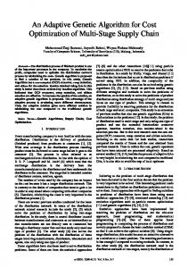
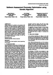
Based on the achievements above and the MS Visual C++, the software package PESO (Pipeline Emulation System and Optimization) has been developed for the practical steady state optimization of gas gathering, transmission and distribution pipeline networks. PESO has an input and output interface in the form of text files and figure files. It allows operators to create a network on the software interface; to receive initial values of supplies, demands and gas parameters; to produce and present a graphic output as shown in Fig.1 and Fig.2. The general functions of optimization are: to minimize the

Figure 3.

© 2011 ACADEMY PUBLISHER

Figure 1. Network creating interface

Figure 2. Results output interface

V.

APPLICATION EXAMPLE

A pipeline network system constructed as Fig.3 and it is formed by 22 segments of pipelines and 21 nodes. Pipe material is TS-52K and X52. The pressures of the system ranges from 2.0MPa to 3.6MPa. The management fees are obtained according to sale price of gas. The structural factors are shown in TABLE I and the input (output) quantity, quantity constrains and purchasing (sale) price of gas of each node are shown in TABLE II. The negative quantities present the input quantities while the positive ones present the output quantities.

Simplified diagram of basic information of a gas pipeline network

JOURNAL OF SOFTWARE, VOL. 6, NO. 3, MARCH 2011

457

TABLE I. BASIC DATA OF EACH SEGMENT Description of pipes

NO.

Pipeline specification 720×8 720×8 720×8 720×8 720×8 720×8 720×9 711×11 720×8

Fitting friction coefficient

Length(km)

1 2 3 4 5 6 7 8 9

1—2 2—3 3—4 4—5 5—6 6—7 7—8 7—8 8—9

0.7 28.5 19.6 16.1 21.2 7.4 1.4 1.4 4.2

0.4 0.011 0.011 0.011 0.011 0.011 0.011 0.011 0.011

10

9—10

720×8

41.5

0.011

11 12 13 14 15 16 17 18 19 20 21 22

10—11 11—12 12—13 13—14 14—15 15—16 16—17 16—17 17—18 18—19 19—20 20—21

720×8 720×8 720×8 720×8 720×8 720×8 720×8 720×8 720×8 720×8 720×8 529×7

32.2 7.3 18.2 34.6 26.9 17 1.7 1.7 1.4 4.6 10 1.2

0.011 0.011 0.011 0.011 0.011 0.011 0.011 0.011 0.011 0.03 0.018 0.018

TABLE II. THE OPTIMIZATION DATA OF EACH NODE NO. 1 3 12 1 2 3 3 4 5 6 6 6 7 8 9 9 10 11 12 12 12 13 14 15 15 16 17 18 19 19 20

Purchasing (Sale) price (Yuan/m3) 0.645 0.645 0.645 1.01 1.0525 1.01 1.00 1.01 1.01 1.0139 0.872 1

1.0516 1 1.0525 1.0523 1.0947 1.0525

1 1.1609

1.01 1.0943 1.0525

Gas consumption (104m3/d) -400 -80 -140 3.90 1.00 17.85 0.31 2.60 0.42 3.60 14.00 2.40 0.0 0.0 2.35 2.00 0.80 0.0 0.87 1.51 8.35 0.0 0.0 4.00 1.50 0.0 0.0 0.0 1.50 4.00 1.19

© 2011 ACADEMY PUBLISHER

Income (104Yuan/d) -256.0 -51.6 -90.3 3.939 1.053 18.029 0.31 2.626 0.424 3.650 12.208 2.40 0.0 0.0 2.471 2.0 0.842 0.0 0.916 1.653 8.788 0.0 0.0 4.0 1.741 0.0 0.0 0.0 1.515 4.377 1.252

Maximum consumption (104m3/d) -400 -80 -140 4.485 1.05 20.5275 0.3255 2.99 0.441 4.14 14.28 2.52 0.0 0.0 2.7025 2.1 0.84 0.0 0.8874 1.5402 8.517 0.0 0.0 4.2 1.575 0.0 0.0 0.0 1.575 4.2 1.2495

Minimum consumption (104m3/d) -400 -80 -140 3.822 0.95 17.493 0.2945 2.548 0.399 3.528 12.6 2.28 0.0 0.0 2.303 1.9 0.76 0.0 0.783 1.359 7.515 0.0 0.0 3.8 1.425 0.0 0.0 0.0 1.425 3.8 1.1305

Optimization consumption (104m3/d) -400 -80 -140 3.822 1.05 19.9093 0.2945 2.99 0.441 4.14 12.6 2.28 0.0 0.0 2.7025 1.9 0.84 0.0 0.8874 1.5402 8.517 0.0 0.0 3.8 1.575 0.0 0.0 0.0 1.51 4.2 1.2495

Optimization pressure (MPa) 3.60 3.535 3.081 3.60 3.598 3.535 3.535 3.475 3.425 3.359 3.359 3.359 3.338 3.334 3.321 3.321 3.200 3.103 3.081 3.081 3.081 2.984 2.791 2.630 2.630 2.525 2.514 2.505 2.470 2.470 2.412

Maximum income (104Yuan/d) -256.0 -51.6 -90.3 3.860 1.105 20.108 0.295 3.020 0.445 4.198 10.987 2.280 0.0 0.0 2.842 1.900 0.884 0.0 0.934 1.686 8.964 0.0 0.0 3.800 1.828 0.0 0.0 0.0 1.525 4.596 1.315

458

JOURNAL OF SOFTWARE, VOL. 6, NO. 3, MARCH 2011

20 20 21 21 21 21 21 21 21 21 21 Total

1.0968 1.0 1.1001 1.0473 1.0884 0.8635 1.1058 0.7643 0.8204 1.1048 1.0

17.00 242.62 18.00 5.14 2.50 4.00 1.33 12.00 140.00 3.26 100

18.646 242.62 19.802 5.383 2.721 3.454 1.471 9.172 114.856 3.602 100.0 198.021

17.85 242.62 18.9 5.397 2.625 4.08 1.3566 12.24 161 3.423 100

According to the data in TABLE II, it can be concluded that gas consumption of each node is optimized because of the different sale price. The gas consumption of node 20 whose sale price is 1.0968 Yuan/m3 was 17 × 104m3/d before and its optimized consumption is 17.85 × 104m3/d so that the income increase 0.932 × 104Yuan/d. On the other side, the gas consumption of node 1 whose sale price is 1.01 Yuan/m3 was 3.9×104m3/d before and its optimized consumption is 3.822×104m3/d so that the income decrease 0.079× 104Yuan/d. The optimization of other nodes is also based on their price. According to the method that increases the consumption of high price node and decreases it of low price node, the overall income of the system increase 1.354 × 104Yuan/d although the overall consumption remains the same. Hence, Operation optimization has accomplished the results of maximizing operation benefit. VI.

16.15 242.62 17.1 4.883 2.375 3.6 1.197 10.8 137.2 3.097 100

19.578 242.62 20.792 5.652 2.857 3.109 1.500 8.254 112.559 3.782 100.0 199.375

This paper is a project supported by 973 arranged subject (No.2006CB705808), sub-project of National science and technology major project of China (No.2008ZX05054) and Scientific Research Fund of Sichuan Provincial Education Department (09ZB097). REFERENCES [1]

[2] [3]

[4]

[5] [6]

[7] [8]

[9] [10] [11] [12] [13]

© 2011 ACADEMY PUBLISHER

2.412 2.412 2.402 2.402 2.402 2.402 2.402 2.402 2.402 2.402 2.402

VII. ACKNOWLEDGMENT

CONCLUSION

In this paper, we presented the gas pipeline network optimization mathematic model. The objective function of the model is the maximum operation benefit and it is established with consideration of quality input (output) constraints of each node, operation pressure constraints of pipelines, compressor constraints, valve constraints and hydraulic constraints of the pipelines system. In order to obtain the global optimal solution, we utilized the adaptive genetic algorithm to solve the large scale nonlinear discrete-continuous optimization problem. Based on the theory achievements, a gas pipeline network simulation and optimization software (PESO) is developed. In the application example, a steady state operation optimization problem is solved. The results show the operation benefit is improved with using of AGA. As a result, AGA is ready for application to other more difficult optimization problems such as the gas network transient optimization. However, the optimal results obtained through AGA should be compared with other heuristic algorithm such as simulated annealing algorithm, artificial neural networks, so that the advantages and disadvantages of AGA can be confirmed.

17.85 242.62 18.9 5.397 2.625 3.6 1.3566 10.8 137.2 3.423 100

C. J. Li, W. L. Jia, and X. Wu, “Comprehensive valuation on regulation schemes of gas transmission pipelines,” ASCE Proceedings of the International Conference on Pipelines and Trenchless Technology, Shanghai, China, pp.581-590, October 2009 Y. Wu, K. K. Lai, and Y.J. Liu, “Deterministic global optimization approach to steady-steady distribution gas pipeline,” Optim.Eng.pp.259-275,July 2007 T. S. Yang., “Development and Application of West-East Gas Steady Flow Operation Optimization Software(in Chinese),” Master's thesis, Petroleum University, Beijing, China, 2002. D.E.Goldberg., “Computer-aided Gas Pipeline Operation Using Genetic Algorithms and Rule Learning,” PHD Dissertation, University of Michigan, Michigan, USA, 1983. V.B. Mantri, L.B. Preston., and C. C. Pringle, “Computer Program Optimizes Nature Gas Pipeline Operation,” Pipeline Industry ,July 1986. Z. Renji, S. Selandari, and H. G. Nicolai., “A System for Control and Optimum Operation of a Gas Transmission Network,” PSIG 19th Annual Meeting, Tulsa, October 1987 Michael J. Ryan, P. B. Percell., “Steady State Optimization of Gas Pipeline Network Operation,” PSIG 19th Annual Meeting, Tulsa, October 1987 W. Tony, G. E. Broadbent., “Optimization in the Operation of Compressor Station on the Moomba to Adelaide Gas Pipeline Network,” PSIG 21th Annual Meeting, 1989. M. A. Renee., “Optimizing Compressor Operation By Effective Application of Performance Models,” PSIG 23th Annual Meeting, Houston , May 1991 S. Bhaduri, R. K. Talachi., “Optimization of Natural Gas Pipeline Design,” ASME Petroleun Dimision,1988. J. G. Wilson, “Optimization of Large Gas Networks,” The European Confercence on Mathematics in Industry, The University of Stranthclyde, Glasgow, August 1988. P, D. Anglard., P. Hierarchical., “Steady State Optimization of Very Large Gas Pipelines,” PSIG 20th Annual Meeting, Toronto, October 1988 Y. Yang., “ Study on Optimization Model of SichuanChongqing natural gas pipe network’s Operational Safety

JOURNAL OF SOFTWARE, VOL. 6, NO. 3, MARCH 2011

and Efficiency Objective(in Chinese),” Doctoral Thesis, August 2008. [14] C. J. Li., Y. Yang.,” Operation Optimization Technology of Natural Gas Pipeline(in Chinese),” Natural Gas Industry, vol.25, No.10, October 2005. [15] M. Srinivas., PATNAIL. “Adaptive Probabilities of Crossover and Mutation in Genetic Algorithms,” IEEE Transaction on System, Man and Cybernetics, Vol.24, No.4, pp. 656-667, 1994.

Changjun Li is superintendent of the oil and gas storage department of Southwest Petroleum University and is also a professor at SWPU, Chengdu, China. He holds an MS degree in oil and gas storage and transportation from SWPU in 1988 . He has been a teacher in SWPU since 1988. He has compiled four monographs, and the typical one is: Gas Transmission Through Pipelines (Beijing, China: Petroleum Industry Press,2008) which is the key teaching material for universities in China. Mr Li is a member of Society of Petroleum (SPE) and China Petroleum Association.

Wenlong Jia is studying for his MS in oil and gas storage and transportation at SWPU, Chengdu. He holds a BS in the same field of study from SWPU in 2008.

Yi Yang is an assistant professor of petroleum engineering at PetroChina, Beijing. He holds a PhD in oil and gas storage and transportation from SWPU(2008).

Xia Wu is studying for his MS in oil and gas storage and transportation at SWPU,Chengdu. He holds a BS in the same field of study from SWPU in 2008.

© 2011 ACADEMY PUBLISHER

459