Hierarchical Simultaneous Localization and Mapping - AFRL

Hierarchical Simultaneous Localization and Mapping Brad Lisien, Deryck Morales, David Silver, George Kantor, Ioannis Rekleitis and Howie Choset Carnegie Mellon University, Pittsburgh, PA 15217 {blisien@, deryck@, dsilver@andrew., kantor@ri., rekleitis@, choset@cs.}cmu.edu

Abstract— This paper presents a novel method of combining topological and feature-based mapping strategies to create a hierarchical approach to simultaneous localization and mapping (SLAM). More than simply running both processes in parallel, we use the topological mapping procedure to organize local feature-based methods. The result is an autonomous exploration and mapping strategy that scales well to large environments and higher dimensions while confronting the issue of obstacle avoidance. We have obtained successful results of our approach in an area spanning 5000 square meters.

I. I NTRODUCTION This paper presents a new method to explore and map large-scale, unknown spaces. With the choice of three basic types of maps: topological, grid-based, and feature-based, it seems that one must settle for drawbacks inherent in each technique in order to take advantage of its particular benefits. Topological techniques scale nicely to large spaces and higher dimensions, but cannot be used to position a robot at an arbitrary location (can only localize to nodes in the topological graph) and generally do not address the problem of obstacle avoidance. Grid-based approaches offer discretized renditions of unstructured free spaces which can be used to localize a robot, but the high resolution required for accurate representations demands large amounts of memory to store and computation time to maintain. Feature-based methods extract distinct landmarks from an environment for use in robot localization but do not explicitly address obstacles unless the obstacles have structured, observable characteristics. Feature and gridbased methods also grow in complexity with the size of the environment in a manner which precludes them from scaling well to large environments and higher dimensions. Our approach is to combine the strengths of a topological map with those of a feature-based map: we use a topological map to decompose the space into regions within which we can build a feature-based map of moderate computational complexity for arbitrary localization. Our contribution is a new hierarchical map where the generalized Voronoi graph (GVG) [4] serves as our high-level topological map organizing a collection of feature-based maps at the lower level. By choosing the GVG as the basis for our topology, we inherit all of its well documented properties. In particular, the GVG offers the ability to safely navigate in the presence of obstacles, a characteristic which feature-based maps lack. Moreover, the GVG embodies an exploration strategy with which we can autonomously and completely chart an environment. We term our approach for exploring

an environment and creating such a map H-SLAM for hierarchical simultaneous localization and mapping. II. BACKGROUND Leonard and Durrant-White [12] first coined the term simultaneous localization and mapping or SLAM; this field has received considerable attention in the last five years and we review some seminal results in Section II-A. One challenge facing the SLAM community is that of computational complexity in large-scale spaces; we address this problem by sub-dividing the free space into smaller regions. This idea is not new and some recent results are reported in Section IIB. We break down the space into regions using the topology of the space with the GVG. We review topological methods in Section II-C. A. Feature-Based SLAM Conventional simultaneous localization and mapping techniques are generally types of feature-based SLAM. This process involves fusing observations of features or landmarks with dead-reckoning information to track the location of the robot in the environment and build a map of landmark locations. The numerous implementations typically include variations on the Kalman filter [18], [7], [10], [16], or particle filters [19], [9]. The extended Kalman filter (EKF) [18], [7] uses a linear approximation of the system to maintain a state vector containing the locations of the robot and landmarks as well as an approximation of correlated uncertainty in the form of a covariance matrix. The EKF has become notorious in terms of the growth of complexity due to the update step requiring computation time proportional to the square of the number of landmarks. This obviously becomes prohibitive in large environments. Each of these feature-based methods has its advantages and disadvantages; however, common to all is the increase in computational complexity with the size of the environment and number of landmarks. A number of techniques have been proposed to alleviate this problem, such as the extended information filter [15], [20], un-scented Kalman filter [10], and fastSLAM [13] but the growth of complexity is inherent in maintaining a global map. B. Sub-mapping Strategies Since the complexity of the global map cannot be avoided, some researchers have proposed dividing the global map into sub-maps, within which the complexity can be bounded. Connections between sub-maps are represented by their

topology of interconnection. Chong and Kleeman [3] introduced a topology of multiple, connected local maps where a new map is started when the variance in robot position grows too large. These locally accurate maps are linked through coordinate transformations between their origins. Bosse et. al. [1] introduced the term atlas to refer to a collection of sub-maps built with a similar method of creating a new map when the uncertainty of the robot location grows above some limit. Simhon and Dudek [17] proposed a strategy to create new maps in the presence of feature rich regions or islands of reliability. On a related note, Thrun [21] uses a topological map to segment a gridbased map into sub-maps as a post-processing step. C. Topological Methods Kuipers and Byun [11] developed a three level hierarchy of control, topology, and geometry with which they simulated an exploration and mapping strategy. The control level determined distinctive places, the topological level tied these distinctive places together, and the geometric level built metric maps around this framework. Nagatani and Choset [5] use the generalized Voronoi graph (GVG) as the topology for their map. Nodes of the GVG are either meet points, the set of points equidistant to three or more obstacles, or boundary points where the distance between two obstacles equals zero. These nodes are connected by edges which are paths of two-way equidistance, see the example in Figure 1. The definition of the nodes and edges automatically induce well defined control laws that allow a robot to trace an edge (either known or unknown a priori) and home onto a meet point. Exploration is achieved by having a robot sequentially traverse unexplored edges emanating from meet points. If the robot encounters a boundary node or a previously visited meet point (i.e., there is a cycle), the robot follows the partially explored GVG to a meet point with an unexplored edge associated with it. When there are no meet points with unexplored edges, the process is complete. Therefore, in addition to prescribing low-level control laws, the GVG also provides an arbitration scheme among the control laws to achieve exploration. Localization with the GVG is trivial when the GVG is a tree: the topology automatically dictates at which node the robot is located. The challenge arrives when there are cycles and the nodes look similar to each other. Here, Nagatani and Choset use the relationships amongst neighboring nodes to localize the robot; this is called topological graph matching. To further enhance the topological matching, Nagatani and Choset also use metric information about the nodes and edges. Dudek et al [8] propose an exploration strategy which maintains a tree of all possible representations of the topological structure to ensure that the correct representation is always present in the exploration tree.

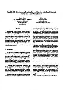
because it is a topological map whose nodes have a definite location in the free space and whose edges not only connect neighboring nodes, but also define paths in the free space. In other words, the GVG is both abstract and embedded in the free space. As such, the GVG is a topological map that induces sensor-based control laws. Each sub-map of the atlas is an edge-map, a local map of one edge referenced from one meet point. Thus for each edge in the GVG there are two edge-maps, one from each meet point. The nodes of the GVG serve as the origins for our edge-maps; thereby tying our local maps both to the topology and to the free space. The edge-maps are formed using a standard extended Kalman filter technique but could be built with any other feature-based approach. The topological mapping occurs concurrently with the feature mapping as we explore and construct the GVG of the environment. For H-SLAM, two levels of data association are required: local and global. The local data association deals with individual landmarks while constructing a single edge-map. Global association compares entire maps of landmarks (i.e., it associates edge-maps) while performing the topologicalSLAM portion of H-SLAM. Edge-matching is simplified because the GVG nodes serve as stable and easily acquired locations for origins of the edge-maps.

Fig. 1. (a) The placement and orientation of edge-map frames are determined by meet points in the GVG. (b) The resulting edge-maps are stored as individual, abstract structures.

III. H IERARCHICAL SLAM The topologies for all of the sub-mapping methods in Section II-B are ad hoc in that any collection of connected entities can be said to have a topology. We wish to set up the atlas to have meaning within the context of the GVG

A. Creating Feature Maps The feature maps are constructed with a standard extended Kalman filter [18]. The locations of the (r)obot

and (l)andmarks are maintained in a state vector X with covariance matrix P where

B. Edge-map Association

(2)

In the previous section we discuss data association for landmarks within a single edge-map. In this section, we consider data association for edge-maps within the entire atlas. In other words, we need a means by which we can determine whether a recently constructed edge-map is new or may already exist. Before we can match two edge-maps, they must first be aligned by associating the individual landmarks between them and determining the offset of the origins. The location of a landmark from the (C)andidate map expressed in the frame of the (E)xisting map can be related through the frame offset Q,  E    xC Qx + xC cos Qθ − yC sin Qθ = . (7) XCE = E yC Qy + xC sin Qθ + yC cos Qθ

where Q represents the uncertainty associated with the odometry input. When a feature is sensed, its measurement must either be associated to an existing feature in the map or it must be added as a new measurement. The location of the robot, along with the locations of landmarks, are used to predict the expected values of range and bearing in a measurement ˆ using the sensor model equation, h(X). The estimate, Z, measurements of range and bearing, Z, are checked against the estimates with a Mahalanobis distance, χ, computed by,

We then implement an extended Kalman filter following a similar outline as in Section II-B. We first associate a landmark location in the candidate frame with the corresponding landmark location in the existing frame using the Mahalanobis distance metric. We use the associated pair as an estimate and a measurement to update the offset, Q, and the uncertainty of that offset. The matching of edge-maps is performed by creating an innovation vector containing all of the differences in landmark position of associated landmarks in the frame of the existing edge. The innovation covariance is simply

−1 χij = (Zi − Zˆj )T Sij (Zi − Zˆj ),

S = PE + GPC GT ,

X=




xr

yr

θr

xl1

yl1

· · · xln

yln

T

. (1)

When the robot is at a meet point and facing the edge departure direction, X and P are initialized to all zeros defining the location of the robot to be at the origin. Every sensor update consists of an odometry measurement and a series of range and bearing measurements to visible point landmarks. The odometry is used as an input, U, to predict ˆ k+1 , according to the state of the robot at the next step, X the state transition equation f (X, U). The corresponding prediction covariance Pˆk+1 is calculated by Pˆk+1 = ∇f Pk ∇f T + Q,

(3)

where Sij is the measurement covariance for the measurement/estimate pair. Each measurement is associated with the existing landmark yielding the minimum distance, provided that this minimum falls below an acceptance threshold. If the smallest χ exceeds a high threshold, meaning that the measurement is extremely unlikely to have been of any existing landmark, then the measurement is used to initialize a new landmark. With a set of range and bearing estimates, we can compute ∇h and the Kalman gain, K = Pˆ ∇hT S −1 .

(4)

The difference between the estimated and measured values, or innovation, is used to compute a state update, ˆ k+1 + K(Z − Z). ˆ Xk+1 = X

(5)

The updated covariance is then given by, Pk+1 = Pˆk+1 − KSK T .

(6)

Once the robot arrives at the terminating meet point, the state vector composes our feature map of landmarks, the final robot location is the location of the end meet point, and the covariance matrix represents the uncertainty in the map. We rotate the map and its covariance matrix through a standard linear transformation to align the x-axis to pass through the terminal meet point. Thus, every aspect of the edge-map’s coordinate frame is completely tied to the GVG.

(8)

where G is composed of rotation matrices on the block diagonal which map the candidate edge covariance matrix into the existing frame. The map innovation and innovation covariance matrix are used to compute a Mahalanobis distance for the edge. If the two edges are a very poor fit and only a few landmarks are associated, the χ will be deceptively small. Therefore, a minimum fraction of the landmarks must be associated in order for the edges to match. While exploring an unknown environment, a match between edges does not give an absolute confirmation that the edges are the same since we must allow for isomorphic edge-maps. Edge matching information is better suited to eliminating non-matching candidates in order to narrow the search pool. Once an edge-map has been positively associated to an existing map, the information in the candidate edge can be used to update the existing map. This is achieved by a standard Kalman update (previously explained) with the innovation vector and corresponding covariance matrix being the same as in the map association step above. The end meet point location is included in this update as a regular landmark. The origin location is not known with certainty but can also be updated with the offset calculated during the alignment step. To update the location of the origin, the locations of all of the landmarks are shifted first to accommodate the change in location of the meet point and then rotated to account for relative change in position of the two meet points.

C. Atlas The generalized Voronoi graph maintains the structure of the atlas by first defining the edge-maps and then representing their interconnections. The edge-maps are defined by the GVG since the edge-map coordinate frames are completely expressed by the nodes of the GVG. Each node contains a list of edges including the nodes to which those edges connect. Any location within the free space can be classified within an edge as a relative location from a meet point. The nodes also contain transformations to the frames of adjacent edges; we can concatenate these transformations to form a global representation of the map. With a global optimization, we can exploit the great deal of redundant data contained in the atlas introduced by cycles and thus refine a global map. D. Path Planning In large environments, it would be impractical to pose path planning problems with start and goal locations in terms of global coordinates. Imagine receiving directions from Pittsburgh to New York City in terms of latitude and longitude. Rather than choose a path heading north-east along whichever back road was heading in the proper direction you would want to access a well-connected interstate to get into the city after which you would leave the highway and ultimately find your destination. The GVG provides this roadmap [2] through the environment and does so as the “safest” route, i.e. the furthest from all obstacles. While tracing between nodes of the GVG there is no need to track the global position of the robot since the path is determined entirely by the topology. If the robot is on the GVG and the goal location is closer than any obstacle, the robot is guaranteed a safe, straight-line path to the goal. In the region of the terminal edge, our edge-map allows accurate localization to determine when to depart from the GVG and then how to track the path of the departure to the goal location referenced from a meet point.

IV. E XPERIMENTAL R ESULTS To implement our technique, we used a Nomadic Scout mobile base outfitted with an on-board embedded computer. A fire-wire camera with an overhead omnidirectional mirror was used to obtain range and bearing measurements to engineered landmarks. Keeping the range and bearing sensor separate from the sonar sensors used for topological navigation highlights the separation of levels in our hierarchical framework. Our experiments were conducted in the corridors of the sixth floor of Wean Hall at Carnegie Mellon University. Visual landmarks in the form of small pink boxes were placed along the walls throughout each hallway as features for the EKF. The robot used a modified version of the arc transversal median method (ATM) [6] to build a local map of obstacles which it used to navigate the GVG by maintaining two-way equidistance. When a third obstacle nears equidistance, the robot invokes a homing control law which drives it to the meet point location determined by its local obstacle map. For the purpose of path planning, we need only store nodes at which a decision must be made. Thus, if the robot determines that the meet point has exactly two non-terminal edges it deems this meet point “weak” and does not store it in the graph. These weak meet points often occur due to doorjambs and corners, see Figure 2, but can also be caused by sensor noise. The subset of the GVG with weak meet points removed is called the reduced GVG (RGVG) [14].

E. Global Localization The atlas generated by H-SLAM is well suited to handle the global localization or “wake-up” robot problem. The goal of global localization is to determine where in the environment a robot is initialized given a map of the environment. This problem is nearly solved by our mapping implementation since we require similar functionality to recognize cycles. To determine in which edge-map the robot is located the robot first accesses the GVG and then follows the GVG edge to a meet point. At the meet point, node information is used to eliminate nodes which are highly improbable matches and generate a list of candidate nodes. The robot also has available to it the sensor log which it gathered while traveling to the node. Reversing this log yields a partial edge-map for the arrival edge which can then be used in an attempt to associate the edges of the candidate nodes and further narrow the pool of contending nodes. If multiple hypotheses still remain, then topological matching must be invoked in order to resolve any ambiguity by matching neighboring nodes.

Fig. 2. corner.

Examples of weak meet points resulting from a doorjamb and

When a meet point is categorized as strong, the robot takes a probing step in each edge direction to enhance the local sensor map. Then the meet point is either verified as strong or discarded as weak. Hence in the diagrams showing the path of the robot, spoke-like motions occur at strong meet points. The graph is used during exploration when the robot reaches a boundary node or returns to a previously existing node; Djikstra’s shortest path search is used to find the closest node with unexplored edge(s) and the robot then retraces the graph it has stored to reach that node and depart on the unexplored edge. When this search determines that all edges have been explored, the exploration is complete and the program terminates. Figure 3 shows the path of the robot as recorded by odometry superimposed on a schematic of the sixth floor of Wean Hall. The robot started the graph from the node at the far right of the figure. The RGVG of the environment

Fig. 3. The path of the robot as calculated by odometry is shown superimposed on a schematic diagram of the sixth floor of Wean Hall. Note the detrimental effects of rotational noise on the odometry. y

which it was located was a candidate match for node 0. It then proceeded to choose the previously explored edge to traverse in an attempt to confirm that it had returned x to its starting location. After the edge was traversed and a new map for the edge was computed, the robot positively matched the previously built edge-map with the newly built edge-map thus resulting in a confirmation of the candidate Fig. 5. An individual edge-map is shown as it is stored abstractly in the node. atlas. Landmark locations are shown as stars with covariance ellipses and We mentioned before that edge matching cannot be used the terminal node location as a cross with the largest uncertainty ellipse. in an unknown environment for absolute confirmation that The covariance ellipses are shown greatly exaggerated for visualization the edge-maps were generated by the same edge. However, purposes. for the loop closing experiment of Figure 6 we exploit contains 13 nodes: 1 four-way meet point, 8 three-way the knowledge that there are no isomorphic edges in the meet points, and 4 boundary nodes. The robot autonomously environment to positively confirm that the loop has been navigated the GVG of the corridors and coordinated all of closed. the path planning to unexplored edges along the GVG. The system was notified when it returned to an already existing meet point through a user interface “oracle” prompt. Once notified, the robot updated the corresponding connections in the graph structure and then planned a path to the nearest unexplored node. When the robot returned to the fourway meet point (node four), it verified that the GVG was complete and then exited successfully. The total length of Fig. 6. The odometric path recorded during a loop closure experiment the path that the robot traversed was 572.1m. is shown on a schematic of the environment. The two locations in the It is important to note that no data were ever recorded odometry corresponding to node zero are noted. in a global frame of reference. Rather, the odometry plots were created by concatenating the reverse transformations V. C ONCLUSION from one frame to another. The resulting feature-maps created during this experiment In this paper, we outlined the potential for hierarchical can be seen in Figure 4 superimposed on the schematic simultaneous localization and mapping in the navigation, of the environment. The figure was generated by tying the exploration, and mapping of large-scale environments and origins of the edge-maps computed by the algorithm to the have proven the effectiveness of H-SLAM in a planar locations of the meet points in the schematic. Near meet environment, by implementation. points, overlapping landmarks can be observed correspondIn its current form, H-SLAM is not a complete solution ing to landmarks which are shared among edges. to all SLAM problems. H-SLAM will not be successful in Figure 4 also shows a coordinate frame for one of the wide-open environments which do not have particularly rich edges embedded in the schematic of the environment. In topologies. This suggests that we need a different high level Figure 5 the same edge is shown as it is stored in the map other than the GVG in such cases. Future work will atlas. For visualization purposes, the uncertainty ellipses are consider developing such a map. shown greatly exaggerated. The key feature of this hierarchical approach to simultaneFigure 6 shows the odometric path of the robot as ous localization and mapping is the meaningful embedding recorded during an experiment to demonstrate how topo- of sub-maps into the free space. Because the GVG has a logical loop closure works. The robot started at node 0 and concrete basis in the free space, we are able to tie our then traced counterclockwise around the outer loop of the edge-maps to the environment and also acquire the ability to environment. When the robot fully traversed the loop, a path autonomously navigate in the presence of obstacles despite length of more than 300m, it recognized that the node at only maintaining a feature map.

Fig. 4. The edge-maps generated during the run of Figure 3 are shown embedded in a schematic of the sixth floor of Wean Hall. Landmark locations are shown as stars with node locations as dark circles. The edge-maps are displayed by tying their origins to the locations of meet points as determined in the schematic.

The complexity of global localization is greatly alleviated by a coarse discretization of the world. However, when the discretization is based on an arbitrary method, such as a square grid, the accuracy of the discrete representation, and thus the localization, is directly related to the resolution of the grid. The GVG offers a coarsely discretized map without any sacrifice in completeness of the representation of the environment or accuracy in localization. The meet points of the GVG offer multiple “entry” points into the atlas. Once an agent has localized itself to a node, it can reference its exact topological location in the atlas as well as have a good characterization of its uncertainty in metric location within a particular edge-map. Looking to multi-robot systems, these entry points offer an excellent method to reconcile either partially of fully completed atlases constructed by different robots. We have shown how the GVG breaks down a planar world for a concise representation. This will be useful when coping with large planar environments but can prove essential when scaling H-SLAM for cluttered three-dimensional environments or higher dimensional configuration spaces while maintaining the ability to track arbitrary location within the free space and the capacity for obstacle avoidance. ACKNOWLEDGMENTS The authors would like to sincerely thank Al Costa for his readily available assistance, and Leanne Crosbie for help with figures and much needed perspective. VI. REFERENCES [1] Michael Bosse, Paul M. Newman, John J. Leonard, and Seth Teller. An atlas framework for scalable mapping. In To appear in: 2003 IEEE International Conference on Robotics and Automation., 2003. [2] J.F. Canny. Constructing roadmaps of semi-algebraic sets i: Completeness. Artificial Intelligence, 37:203–222, 1988. [3] K S Chong and L. Kleeman. Large scale sonarray mapping using multiple connected local maps. In International Conference on Field and Service Robotics, pages 538–545, December 1997. [4] H. Choset and J.W. Burdick. Sensor Based Planning, Part II: Incremental Construction of the Generalized Voronoi Graph. In Proc. IEEE Int. Conf. on Robotics and Automation, Nagoya, Japan, 1995. [5] H. Choset and K. Nagatani. Topological simultaneous localization and mapping (slam): toward exact localization without explicit localization. IEEE Transactions on Robotics and Automation, 17(2):125–137, Apr. 2001. [6] H. Choset, K. Nagatani, and N. Lazar. The Arc-Transversal Median Algorithm: an Approach to Increasing Ultrasonic Sensor Accuracy. In Proc. IEEE Int. Conf. on Robotics and Automation, Detroit, 1999.

[7] G. Dissanayake, S. Clark P. Newman, H. Durrant-Whyte, and M. Csorba. A solution to the simultaneous localization and map building (slam) problem. IEEE Transactions on Robotics and Automation, 17(3):229–241, June 2001. [8] Gregory Dudek, Paul Freedman, and Souad Hadjres. Using multiple models for environmental mapping. Journal of Robotic Systems, 13(8):539–559, Aug. 1996. [9] D. Fox, S. Thrun, F. Dellaert, and W. Burgard. Particle filters for mobile robot localization. In A. Doucet, N. de Freitas, and N. Gordon, editors, Sequential Monte Carlo Methods in Practice. Springer Verlag, New York, 2000. [10] S. Julier and J. Uhlmann. A new extension of the kalman filter to nonlinear systems, 1997. [11] B. Kuipers and Y.-T. Byun. A robot exploration and mapping strategy based on a semantic hierachy of spatial representations. Robotics and Autonomous Systems, 8:46–63, 1991. [12] J. J. Leonard and H.F. Durrant-Whyte. Simultaneous Map Building and Localization for an Autonomous Mobile Robot. In IEEE/RSJ International Workshop on Intelligent Robots and Systems, pages 1442–1447, May 1991. [13] M. Montemerlo, S. Thrun, D. Koller, and B. Wegbreit. FastSLAM: A factored solution to the simultaneous localization and mapping problem. In Proceedings of the AAAI National Conference on Artificial Intelligence, Edmonton, Canada, 2002. AAAI. [14] K. Nagatani and H. Choset. Toward Robust Sensor Based Exploration by Constructing Reduced Generalized Voronoi Graph. In IEEE/RSJ Int. Conference on Intelligent Robots and Systems, pages 1687–1698, Seoul, Korea, Nov 1999. [15] E.W. Nettleton, P.W. Gibbens, and H.F. Durrant-Whyte. Closed form solutions to the multiple platform simultaneouslocalisation and map building (slam) problem. In Bulur V.Dasarathy, editor, Sensor Fusion: Architectures, Algorithms,and Applications IV, volume 4051, pages 428–437, 2000. [16] Stergios I. Roumeliotis and George A. Bekey. Bayesian estimation and kalman filtering: A unified framework for mobile robot localization. In Proc. 2000 IEEE International Conference on Robotics and Automation, pages 2985–2992, San Francisco, California, April 22-28 2000. IEEE. [17] Saul Simhon and Gregory Dudek. A global topological map formed by local metric maps. In IROS, volume 3, pages 1708–1714, Victoria, Canada, October 1998. [18] R. Smith and P. Cheeseman. On the representation and estimation of spatial uncertainty. International Journal of Robotics Research, 5(4):56–68, Winter 1986. [19] S. Thrun, D. Fox, and W. Burgard. A probabilistic approach to concurrent mapping and localization for mobile robots. Machine Learning, 31:29–53, 1998. also appeared in Autonomous Robots 5, 253–271 (joint issue). [20] S. Thrun, D. Koller, Z. Ghahramani, H. Durrant-Whyte, and Ng. A.Y. Simultaneous mapping and localization with sparse extended information filters. In J.-D. Boissonnat, J. Burdick, K. Goldberg, and S. Hutchinson, editors, Proceedings of the Fifth International Workshop on Algorithmic Foundations of Robotics, Nice, France, 2002. Forthcoming. [21] Sebastian Thrun. Learning metric-topological maps for indoor mobile robot navigation. AI Journal, 99:1:21–71, 1998.