example, it can be safely concluded that your home thermostat does not need the same type of control as ..... Figure 2: Simple Spacecraft with Four Solar Panels.
AIAA Guidance, Navigation and Control Conference and Exhibit 18 - 21 August 2008, Honolulu, Hawaii
AIAA 2008-6782 1
Adaptive Output Feedback Control as Applied to the Rigid Body Equations of Motion
Downloaded by Eric Mehiel on September 11, 2015 | http://arc.aiaa.org | DOI: 10.2514/6.2008-6782
Rushabh C. Patel and Eric A. Mehiel California Polytechnic State University, San Luis Obispo, CA 93407
A varied method for producing adaptive control is developed in this paper. It involves developing a simplified version of the current Nonlinear Direct Model Reference Adaptive Control (NDMRAC) method. This simplified model of NDMRAC is called Adaptive Output Feedback (AOF) Control. Both types of controllers have varying applications, but in this paper the AOF controller was applied to control the rigid body equations of motion. It was realized that the AOF controller could have an advantage over the NDMRAC controller in the sense of ease of implementation, and also in being better in computational expense. The adaptive method was found to perform better than the standard Full State Feed Back (FSFB) method in this application in the aspect of system response and settling time. The adaptive method was particularly better in the cases when the system being controlled was instantaneously changed during simulation. The adaptive method compensated for the system change with little too no change in trajectory or settling time whereas the FSFB method deviated in both. Control systems of some form can be found in most autonomous systems. The type of control that is used in a system varies primarily on the need for robustness or ease of implementation for the given application. For example, it can be safely concluded that your home thermostat does not need the same type of control as the auto pilot for a fighter jet. This is the reason why there are different types of controllers and many sub-variations of each type of controller. Each one although not necessarily as wide in applicability as the example given, still gives the engineer options in picking a controller that is best suited for the task at hand. With that in mind, this paper takes a look at a type of adaptive control in application to the rigid body equations of motion. The developed controller and the one it is drawn from may or may not be more suited for this particular application, but still add a new potential selection for the engineer in another application. Adaptive control methods are getting more attention since they attempt to deal with new complex control scenarios in an efficient way. Each type of adaptive controller is different in its own way, but fundamentally each one tries to compensate for a system which is dynamically changing, unknown, or even random (in stochastic applications), in an adaptive way. Within adaptive control there exist various subdivisions of the theory. The main classifications of adaptive control fall under direct adaptive control, indirect adaptive control, and robust adaptive control. The indirect adaptive method relies on approximating the plant online, which the controller then adapts too. This system can become very computationally expensive when the order of the plant gets too big in larger systems. Direct adaptive control (DAC) is different in that it requires little to no knowledge of how the plant changes with time, but instead relies on trying to adaptively track the output of a user defined reference model. Indirect adaptive control although more computationally expensive is still a major source of research and types of it can be found in application. It relies on, as mentioned before, on the online identification of the plant. The plant originally was assumed to change slowly with time, but was extended by Tsakalis and Ioannou1 for faster changing plants, which extends its application range. Ruznik, Guez, Bar-Kana, and Steinberg 2 use a combination of plant identification and also gain scheduling in an optimal way to perform better than any one method can by itself to control aircraft dynamics. Yu3 uses indirect adaptive control for pole placement in correlation with a recursive least squares algorithm as a means of robust control. Yoshiaki, Takashi, and Keietsu4 developed a method for disturbance accommodation using an indirect method in which they use the plant and sensor values of the system to adaptively adjust the disturbance accommodation parameters online. This concludes the discussion of indirect MRAC theory as this paper is focused on a type DAC theory, the indirect method will no longer be mentioned. In DAC theory there are different variations, although the fundamental principle behind all of them is that they track a reference model. The different types include Model Reference Adaptive Control (MRAC), Simple Adaptive Control (SAC) and Robust Adaptive Control (RAC), Direct Model Reference Adaptive Control
Copyright © 2008 by Eric A. Mehiel. Published by the American Institute of Aeronautics and Astronautics, Inc., with permission.
Downloaded by Eric Mehiel on September 11, 2015 | http://arc.aiaa.org | DOI: 10.2514/6.2008-6782
2 (DMRAC), and newly the Model Reference Adaptive Iterative Learning Control (MRAIL). Narendra5 was one of the first to develop MRAC for use for MIMO systems. He shows stability for this system using the Lyapunov Stability Analysis, through which he shows that the plant must be Strictly Positive Real (SPR) (More on SPR can be found in Appendix A). SAC and RAC are similar to the fundamental MRAC method in that they require the plant to be SPR, but are different in how they structure the gains. Within these two methods, SAC and RAC differ from each other in that the RAC model adds a feed forward term in order to “add more robustness to the system”, but it can be used to make a non SPR plant to be SPR. The SAC controller is applied by Bar-Kana and Kaufman6 to Large Flexible Space Structures and then is turned into a RAC controller once they add a feed-forward compensator to compensate for the non SPRness of the system due to the limited sensors and actuators in the system. This is also done by Laniando, Bar-Kana, and Kreindler7 in applying RAC to a robotic arm. MRAIL control adds to MRAC by adding an iterative learning controller (ILC) for cases where repetitive tasks are performed. The new system bounds the error of the system to a finite region as the iterations approach infinity. Tayebi8 applies it to a SISO system, but shows the proof for MIMO systems using the Lyapunov Theorem. DMRAC theory, which is the type of control used in this paper, adds to the MRAC method in that the reference model can be of a lower order than the plant. The DMRAC controller also employs the use of a Command Generator Tracker (CGT) which was first developed by Brousard and O’Brien9. Ozelick and Kaufman10 expanded on the CGT by adding a feed forward term that allows the plant to be compensated for if it is not SPR. This new SPR system is called Almost SPR or ASPR. Originally this was the case for SISO systems only, but was later expanded for MIMO systems as well, and shown to be stable using Lyapunov Stability Analysis by Ozelick and Kaufman11. DMRAC has been used by Mehiel12 to control a Deployable Optical Telescope (DOT). In this case the plant can be fairly large order so a lower order reference model is used to allow the tracking of the system. Harvey and Balas13 apply NDMRAC theory to plug and play satellites, a scenario where the inertia of the system can change in numerous ways depending on components attached. This is a perfect application of this type of controller, as now only one controller has to be designed instead of a new one for each satellite configuration. II. AOF Control Theory The proof of AOF control theory follows both that of Torres14 and Mehiel12 for NDMRAC and DMRAC controllers respectively. A model of the AOF system is shown below in Figure 1. CGT
Reference Model
Adaptive Error Gain Plant Figure 1: Simple Nonlinear Model Reference Adaptive Controller
Consider the Nth order nonlinear system represented as
x& p = A p x p + B p u p + f (x p )
(1)
y p = Cp x p where
f (x p ) represents the nonlinear portion of the controller, A p ∈ R N × N , and u p , y p ∈ R M (i.e. the system is
square). This system is considered output feed back stable if there exist some Ge* such that the control law
(
)
u p = Ge* y p such that the system A p − B p Ge* C p is exponentially stable. Now consider the Mth order reference model described by
3 x& m = Am x m + Bm u m + g ( x m )
(2)
y m = Cm x m where g ( x m ) is the non-linear part of the reference model and Am ∈ R
M ×M
. Note that the size of the reference
model is independent of the size of the system model, so can be made lower in order than the system in eq.1. The reference model is stable and therefore bounded, or can be made stable since it is determined by the user. Next the Command Generator Tracker (CGT) is presented. The CGT is at least stable, and determines the inputs for the reference model.
x& q = Aq x q
(3)
Downloaded by Eric Mehiel on September 11, 2015 | http://arc.aiaa.org | DOI: 10.2514/6.2008-6782
u m = Cq x q Next consider an ideal system
x& ∗ = A∗ x ∗ + B∗ u ∗ + f ( x ∗ )
(4)
y ∗ = C∗ x ∗
which is the same order as the plant. This system represents the ideal trajectories of the Plant model. The ideal system is designed so that it theoretically tracks the reference model perfectly such that y = y for all t f 0 . If m
∗
the ideal system tracks the reference model for t f 0 then that implies that the reference model can be made up of some linear combination of the ideal system.
[
x ∗ = S11∗
]
⎧x ⎫ S12∗ ⎨ m ⎬ . ⎩u m ⎭
(5)
If the derivative of the above equation is taken and like terms are solved for then the following conditions directly follow.
Ap S11* = S11* Am , Ap S12* Cq = S11* BmCq + S12* Cq Aq , f (x∗ ) = S11* g (x m ),
(6)
C S = Cm , * p 11
C p S12* Cq = 0. These conditions are suitably called the matching conditions. If the Plant, Reference, and Tracking model satisfy the matching conditions for some Sij then the system is called Totally Consistent. Next the output error, and the state error of the system are respectively defined as
ey ≡ y p − ym ,
(7)
e ≡ x p − x* .
(8)
That concludes the setup of the AOF, and now we will continue by showing this system is stable using the Lyapunov Method in correlation with Barbalat’s Lemma. Theorem 3.1:
4
(
)
If A p + B p G e C p , B p , C p is SPR and the system of equations given by (1), (2), and (3) are totally consistent *
with the adaptive gain of the controller given as T G& e = −e y e y H
where H
(9)
∈ ℜ M ×M > 0 , and the control law for the system given as u p = Ge e y ,
(10)
then the closed loop system is asymptotically stable with the output error of the system going to zero, as t → ∞ .
Downloaded by Eric Mehiel on September 11, 2015 | http://arc.aiaa.org | DOI: 10.2514/6.2008-6782
Proof: We must show that the system is asymptotically stable with the given adaptive gain parameter. First we start by taking the derivative of the state error and combine terms which results in the equation
e& ≡ A p e + B p Δu + Δf where Δu = up-um and
(11)
Δf = f (x p ) - g (x m ) . Next after some further expansion and manipulation the state error
equation becomes reduced to
(
)
e& = A p + B p Ge∗ C p e + B p w + Δf
(12)
ΔG = Ge − Ge∗ and z ≡ e y . Now let Ac = (Ap + B p Ge∗C p ) , then the system reduces to
where w ≡ ΔG z ,
T
e& = Ac e + B p w + Δf .
(13)
Next define the Lyapunov function as
V1 = 12 e Pc e T
(14)
where Pc is positive definite. Taking the derivative of the Lyapunov function we get T T V&1 = 12 e& Pc e + 12 e Pc e& T T T V&1 = 12 e AcT Pc + Pc Ac e + w B Tp Pe c + e Pc Δf T T T V& = − 1 e Q e + e w + e P Δf .
(
1
)
c
2
y
(15)
c
The last step in the derivative is simplified using the Kalman-Yacubovic (K-Y) conditions which can be found in Appendix A. These conditions can be applied since (Ac,Bp,Cp) is SPR. Next we define a second Lyapunov function of the form
(
)
V2 = 12 tr ΔGH −1 ΔG T .
(16)
Taking the derivative of this Lyapunov function results in
(
)
(
V&2 = 12 tr ΔG& H −1 ΔG T + 12 tr ΔGH −1 ΔG& T V&2 = tr ΔG& H −1 ΔG T .
(
)
)
(17)
5
Since
ΔG& = −e y z H , the second Lyapunov reduces to T
T
T V&2 = −e y w .
(18)
Now we combine the two Lyapunov functions, eq.15 and eq.18, to get
V& = V&1 + V&2 T T V& = − 12 e Qc e + e Pc Δf
(19)
Downloaded by Eric Mehiel on September 11, 2015 | http://arc.aiaa.org | DOI: 10.2514/6.2008-6782
We must now show that this function is at least negative semi-definite. First we take the norm of the non-linear term to produce T T V& ≤ − 12 e Qc e + e Pc Δf .
(20)
An upper bound on the non-linear term given as e Pc Δf T
≤ e
T
Pc Δf
T T V& ≤ − 12 e Qc e + e Pc Δf
(21)
Next the non-linear term needs to be bounded. To do this the Lipschitz condition (Appendix A) is applied to the non-linear portion.
The Lipschitz condition gives that
f (x p ) − f (x∗ ) ≤ L x p − x∗ . Which reduces to
Δf ≤ L e . The first derivative now has the form T T V& ≤ − 12 e Qc e + e Pc L e .
(22)
Next we place an upper bound on the error given by e Qc e ≥ σ (Qc ) e T
2
, where
σ (Qc )
is the smallest singular
value of Qc such that − e Qc e ≤ −σ (Qc ) e . Now the derivative of the Lyapunov has the form 2
T
2 T V& ≤ − 12 σ (Qc ) e + e Pc L e .
(23)
To make sure the system is truly bounded, an upper bound is taken on Pc and the error terms are factored out of the equation to get
(
2 V& ≤ − e σ (Qc ) − 2σ (Pc )L
where
)
σ (Pc ) is the largest singular value of Pc such that Pc ≤ σ (Pc ) .
(24) Setting the value in the parenthesis to less
than zero and solving for the Lipschitz constant gives
L≤
σ (Qc ) 2σ (Pc )
(25)
6 which if satisfied will give the system as bounded. Now that we know the error is bounded, as are
QC and PC
since they are constant and positive definite, the error must now be shown to be asymptotically stable. First we must take the second derivative of the Lyapunov function which gives T T T V&& = −e Qc e& + e& Pc Δf + e Pc Δf& .
(26)
The next step is to make sure that the derivative of the error is bounded. In order to show this we start by taking the norm of the error derivative term from eq.13 which gives
Downloaded by Eric Mehiel on September 11, 2015 | http://arc.aiaa.org | DOI: 10.2514/6.2008-6782
e& = Ac e + B p w + Δf .
(27)
It is apparent that the derivative of the error is bounded since we already have shown that the error term is bounded, and so is the non-linear portion of the controller as shown in the first derivative of the Lyapunov function, we now substitute eq.27 into eq.26 to get T T T V&& ≤ e& Qc e + e& Pc Δf + e Pc Δf& .
(28)
The only thing that remains is the derivative of the nonlinear portion, but the derivative of the non-linear portion is dependent from system to system. Since the system is chosen by the user it is assumed that the system will be chosen such that its derivatives are bounded. The system defined in this paper is a rigid body spacecraft, and since the controller itself is physically bounded (i.e. the torque added to the system) and also since the derivative of the nonlinear component is a function of the states which were shown to be bounded, this then implies that the derivative of the nonlinear portion of the controller is also bounded. Since the second derivative of Lyapunov is bounded then the first derivative is continuous, and therefore by Barbalat’s lemma since the first Lyapunov function is finite, as shown by the first derivative, then the first derivative approaches zero as t → ∞ . This means the error goes to zero as time approaches an infinite value. III. Equations of Motion and Control Law The spacecraft rigid body equations of motion are presented here along with the control law for convenience. The derivations can be found in both Sidi15 and Wie16. First we start with Euler equations for momentum of a rigid body which are given by
v v v v v M = h&I = h& + ω × h r&
(29)
r
r
& , where w is angular velocity. Next the quaternion Where h is the angular momentum which is equivalent to Jw dynamics are determined so that the rigid body position can be known for the control law. These quaternion dynamics are developed in both Sidi15 and Wie16. They are derived from the derivative of the relationship between the Euler angles and the quaternion to produce
v v v v 1 q& = (q 4ω − ω × q ), 2 1 v v q& 4 = − ω T q. 2
(30)
The control law for the rigid body spacecraft is a closed loop controller which distributes torques according to a weighting between the quaternion error and angular velocity. It is given by
r r r M = − Kqe − Cω .
r The q e term is the quaternion error and is the equivalent of a rotation.
(31)
7 An important thing to note for writing the control law for the adaptive controller is that the same Torque distribution that is used for the closed loop system is applied to the adaptive control inputs, with the exception that the signs are reversed. Keeping this in mind, the adaptive input goes into the control law
r ~, M = Kq~ + Cw ~⎤ ⎧⎪e yw ⎫⎪ ⎡w ⎢ q~ ⎥ = [Ge ]⎨ e q ⎬ = Ge e y , ⎪⎩ y ⎪⎭ ⎣ ⎦
(32)
Downloaded by Eric Mehiel on September 11, 2015 | http://arc.aiaa.org | DOI: 10.2514/6.2008-6782
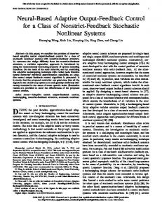
for the AOF system. When determining the K and C gains for the controller use those values which were developed for the closed loop feedback system. The K and C gains are kept in the adaptive portion because if the gains were not there then the system would no longer be a square system, which is part of the requirements of the proof. An important observation in the adaptive method design is that we are controlling the torque using the state quaternion error and state angular velocity error as shown in eq.29. The state quaternion error portion is much different than the quaternion error which is used in the FSFB control scheme. The state error is merely a difference whereas the quaternion error is actually a rotation. The quaternion error currently cannot be brought into this control scheme due to the affects that it has on the stability proof of both the NDMRAC and AOF control theories. However to see an example of quaternion error being used in a different adaptive control scheme, Costic, Dawson, Quieroz, and Kapila18 is a good source. Keep in mind that they actually use the equivalent of quaternion error by using the difference of the Euler angle states. Even though this can be effective, even for the NDMRAC and AOF controllers, it defeats the purpose of using quaternions, which is to avoid the singularity issues with Euler angles. IV. Simulation of FSFB and AOF To give an accurate comparison of the capabilities of each of the controller, all the controllers will have responses as similar to each other as possible for a simple quaternion maneuver. The inertia matrices will then be changed in mid simulation to see how each controller responds. The inertia matrix chosen is based off the geometry already shown in Figure 2.
Figure 2: Simple Spacecraft with Four Solar Panels
The
FSFB
response
is
qi = [0.45 0.45 0.45 seen below in Figure 3.
first
tested for the system to go from an initial quaternion of 0.6265 to a command quaternion of q c = 0 0 0 1 . The responses can be
]
[
]
8
quaternion 2
0.4
0.4
0.3
0.3 q2
q1
quaternion 1
0.2 0.1 0 0
0.2 0.1
20 40 time(sec) quaternion 3
0 0
60
20 40 time(sec) quaternion 4
60
20 40 time(sec)
60
1 0.4
0.9 q4
0.2
0 0
0.8 0.7
0.1 20 40 time(sec)
60
0
Figure 2: FSFB Quaternion Response
Figure 3 shows that the quaternion response of the system settles just after 50 seconds. The angular velocity responses are seen below in Figure 3, and reconfirms that the system settles in approximately 50 seconds.
rad/sec
rad/sec
Angular Velcoity (wx)
rad/sec
Downloaded by Eric Mehiel on September 11, 2015 | http://arc.aiaa.org | DOI: 10.2514/6.2008-6782
q3
0.3
0 -0.02 -0.04 -0.06 -0.08 0
10
20
30 40 time(sec) Angular Velcoity (wy)
50
60
0 -0.02 -0.04 -0.06 -0.08 0
10
20
30 40 time(sec) Angular Velcoity (wz)
50
60
0 -0.02 -0.04 -0.06 -0.08 0
10
20
50
60
30 time(sec)
40
Figure 3: FSFB Angular Velocity Responses
Now the AOF is simulated for the same command quaternion and ICs. Its quaternion responses are seen below in Figure 4.
9
quaternion 2
0.4
0.4
0.3
0.3
q2
q1
quaternion 1
0.2 0.1 0 0
0.2 0.1
20 40 time(sec) quaternion 3
0 0
60
20 40 time(sec) quaternion 4
60
20 40 time(sec)
60
1
q4
q3
0.9
0.3 0.2
0 0
0.8 0.7
0.1 20 40 time(sec)
60
0
Figure 4: AOF Quaternion Responses
The quaternion responses for the AOF are almost identical to that of the FSFB system. Next the angular velocities are observed for AOF in Figure 5, and it again follows closely to the FSFB system. Angular Velcoity (wx) rad/sec
0 -0.05 -0.1 0
10
20
30 40 time(sec) Angular Velcoity (wy)
50
60
10
20
30 40 time(sec) Angular Velcoity (wz)
50
60
10
20
50
60
rad/sec
0 -0.05 -0.1 0
0 rad/sec
Downloaded by Eric Mehiel on September 11, 2015 | http://arc.aiaa.org | DOI: 10.2514/6.2008-6782
0.4
-0.05 -0.1 0
30 time(sec)
40
Figure 5: AOF Angular Velocity Responses
Now an inertia (decrease) change is introduced to test the robustness of each system to the given change. The inertia matrix is changed to represent the geometry of Figure 6.
10
This is a situation in which the spacecraft loses two of its solar panels somehow (collision, bombardment, etc.). The remaining solar panels are also rotated so that the inertia matrix is slightly more skewed. The change of inertia takes place at 15 seconds into the simulation. The FSFB quaternion response for this system is shown in Figure 7. As seen from the responses, the system settles at a little after 77 seconds. quaternion 2
0.4
0.4
0.3
0.3 q2
q1
quaternion 1
0.2 0.1 0 0
0.2 0.1
20
40 60 time(sec) quaternion 3
0 0
80
20
40 60 time(sec) quaternion 4
80
20
40 60 time(sec)
80
1 0.4
0.9 q4
0.3 q3
Downloaded by Eric Mehiel on September 11, 2015 | http://arc.aiaa.org | DOI: 10.2514/6.2008-6782
Figure 6: Simple Spacecraft with 2 Solar Panels
0.2
0.7
0.1 0 0
0.8
20
40 60 time(sec)
80
0
Figure 7: FSFB Quaternion Responses with Inertia Change
This shows how robust the FSFB controller can actually be. Next the angular velocities are observed as seen in the Figure 8.
11
rad/sec
10
20
30 40 time(sec) Angular Velcoity (wy)
50
60
0 -0.02 -0.04 -0.06 -0.08 0
10
20
30 40 time(sec) Angular Velcoity (wz)
50
60
0 -0.02 -0.04 -0.06 -0.08 0
10
20
50
60
30 time(sec)
40
Figure 8: FSFB Angular Velocity Responses with Inertia Change
The angular velocities for the FSFB system experience an impulse as expected when the inertias are changed, but then settle right after with no apparent transients to note. Next the AOF quaternion responses are observed in Figure 9. quaternion 2
0.4
0.4
0.3
0.3 q2
q1
quaternion 1
0.2 0.1 0 0
0.2 0.1
20 40 time(sec) quaternion 3
0 0
60
20 40 time(sec) quaternion 4
60
20 40 time(sec)
60
1 0.4
0.9
0.3
q4
q3
Downloaded by Eric Mehiel on September 11, 2015 | http://arc.aiaa.org | DOI: 10.2514/6.2008-6782
rad/sec
rad/sec
Angular Velcoity (wx) 0 -0.02 -0.04 -0.06 -0.08 0
0.2
0.7
0.1 0 0
0.8
20 40 time(sec)
60
0
Figure 9: AOF Quaternion Responses with Changing Inertia
It is seen that the quaternion values actually settle at close to the same time and follow the same response as the case with no inertia change. This is the desired response of the AOF controller. Next the angular velocities are observed in Figure 10.
12
Angular Velcoity (wx) rad/sec
0 -0.05 -0.1 0
10
20
30 40 time(sec) Angular Velcoity (wy)
50
60
10
20
30 40 time(sec) Angular Velcoity (wz)
50
60
10
20
50
60
rad/sec
0 -0.05
rad/sec
0 -0.05 -0.1 0
30 time(sec)
40
Figure 10: AOF Angular Velocity Responses with Changing Inertia
The angular velocities for the AOF take the change in inertia very well, with little change from the original trajectory. In fact the change is barely noticeable. A closer look at the trajectories at the time of change is shown in Figure 11. Angular Velcoity (wx) rad/sec
-0.03 -0.032 -0.034 14.98
14.99
15
15.01 15.02 time(sec) Angular Velcoity (wy)
15.03
15.04
14.99
15
15.01 15.02 time(sec) Angular Velcoity (wz)
15.03
15.04
14.99
15
15.03
15.04
rad/sec
-0.03 -0.032 -0.034 14.98
-0.03 rad/sec
Downloaded by Eric Mehiel on September 11, 2015 | http://arc.aiaa.org | DOI: 10.2514/6.2008-6782
-0.1 0
-0.032 -0.034 14.98
15.01 time(sec)
15.02
Figure 11: Close Up of Angular Velocity Responses at Time of Inertia Change
13 The AOF damps out the change in inertia for
ωx
and ω y , and
ωz
almost instantaneously. This response is the
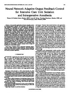
desired result that we expect of an adaptive system, since it forces the actual system to track a reference model which is unaware of any system change. Next, the adaptive gain responses for the inertia change can be observed in Figure 12. The two gains which are observed were arbitrarily picked from the 49 element adaptive error gain matrix. As can be seen, the gains for the system appear not to have any change when the systems inertia is changed at 15 seconds. This is because the gains become so large, even before the inertia change, that at the time of change the small difference that may occur in the gains is unnoticeable. Adaptive Error Gain Response 2500
Arb. Gain 1 Arb. Gain 2 1500 Gain Value
Downloaded by Eric Mehiel on September 11, 2015 | http://arc.aiaa.org | DOI: 10.2514/6.2008-6782
2000
1000
500
0
-500 0
10
20
30 time(sec)
40
50
60
Figure 12: Adaptive Error Gain Responses for AOF
Looking at all the controllers, it is obvious that in the sense of robustness, the AOF controller is definitely more robust than at least the FSFB controller for rigid body motion. A look at the computational time for each of the simulations using each controller in Table 1 shows that the AOF computational time does increase slightly when the inertia is decreased, but this is believed to be attributed to the ode45 algorithm in MatLab. It is also partly due to how the inertia matrix changes. If simply scaled, then the computational time decreases dramatically.
Inertia Change No Change Decrease FSFB
0.36
0.484
AOF
1.95
15.562
Table 1: Simulation Run Times for Each Controller (settling time included) (seconds)
The FSFB controller is even less computationally expensive than the AOF controller, but lacks obvious robustness in certain applications as can be seen in both the settling times as well as the cost function values for each controller in Table 2 and Table 3, respectively.
14
Inertia Change No Change
Decrease
FSFB
49.89
77.12
AOF
50.148
50.177
Table 2: Settling Times of Each Controller with Varying Inertias (seconds)
The AOF controller tracks the desired response very well, and so settles at the same time regardless of change in the system. The AOF also performs this action in an optimal way. In order to validate this the cost function
Downloaded by Eric Mehiel on September 11, 2015 | http://arc.aiaa.org | DOI: 10.2514/6.2008-6782
J = ∫ u T Qu
(33)
is used to compare the controller efforts, and the value of the cost functions can be seen in Table 3. Even though it is adapting to the quaternion state error and not the actual quaternion error, the cost function still has similar values to the FSFB system for when the inertia does not change. Since the original trajectories are not exactly the same, the cost function values will differ slightly, as will the controller efforts which are also shown in Table 3. Comparing the various system changes of each controller on the cost values shows that, while the FSFB system deviates from its original cost function values, the AOF controller stays remarkably consistent. Inertia Change No Change
Decrease
FSFB
2.6686/.00033239
2.7096/.00031952
AOF
2.6062/.00043198
2.6062 /.00042012
Table 3: Total /Controller Cost Value of Each Controller with Varying Inertias
In summary, although the AOF controller is more computationally expensive, it outperforms both the FSFB controller in the aspect of system response and settling time. It should also be noted that even though the AOF uses quaternion state error instead of true quaternion error, the controller efforts are still fairly similar to the FSFB system. Knowing all of this it leaves the final decision up to the engineer, depending on what is more needed in any given application, a computationally inexpensive system which does not need to handle much change, or a slightly more expensive system that can. V. Conclusion
This work was intended to develop a simplified version of the NDMRAC controller as a new alternative with similar robustness. This was accomplished in the development of the AOF control method, and was shown to be asymptotically stable. Once the controllers were properly established, each was simulated and the run time was recorded for both changing and non-changing inertias to determine the comparative robustness and complexity of each controller. The simulations were first run for a basic trajectory, then for the case where the inertia decreases at 15 seconds into the simulation. Each controller had good performance, and it was not the case that any of the controllers actually went unstable. The AOF controller was found to perform better in settling time and system response than the FSFB controller. Given the results there is no doubt that the AOF’s adaptive properties could be used and applied to at least the given application in this paper. The adaptive controller is definitely robust and adds much ease in how the plant is defined. The FSFB controller ended up being excellent choice for this application, and actually performed much better than expected even though it violated the inertia-gain relationship of the Lyapunov theory predicted (Wie16) for this non-linear system. Each controller has advantages and disadvantages, so therefore it is in the end, up to the engineer to decide what is more important to their given design. The AOF method although robust is more complicated to design, determine gains for that will satisfy the users desired responses, and computationally expensive whereas this is not the case for the FSFB controller. Within the two adaptive methods though, the AOF method is slightly less computationally expensive, uses less controller effort for a decreasing inertia system, and
15
Downloaded by Eric Mehiel on September 11, 2015 | http://arc.aiaa.org | DOI: 10.2514/6.2008-6782
would also be easier to implement on a real system than an NDMRAC controller. The other obvious advantage is that the user does not have to worry about deviations from the response once the system is designed where in the case for FSFB you do. This could be accounted to some degree if a tracking component was added to the FSFB system. Good system tracking is a process perfectly suited for space applications where pointing and maneuvering is critical to mission success, and deviation from a desired trajectory is an unwanted scenario. This would be a complicated problem for FSFB control accommodate for, especially on spacecrafts that have large frequently moving appendages. The FSFB system must be redesigned most times the system is changed if some form of tracking is not included. It ends up being a function of how much complexity the user expects in the life of the system that they are designing for.
16
Downloaded by Eric Mehiel on September 11, 2015 | http://arc.aiaa.org | DOI: 10.2514/6.2008-6782
List of References 1. Tsakalis, Kostas S. and Ioannou, Petros A., “A New Indirect Adaptive Control for Time-Varying Plants” IEEE Transactions on Automatic Control, Vol. 35 No.6, June 1990: 697 – 705 2.
Ilan Ruznik, Allon Guez, Izhak Bar-Kana, and Marc Steinberg, “online identification and control of Linearized aircraft dynamics”, IEEE AES Magazine, July 1992.
3.
Wen Shyong Yu, “An indirect adaptive pole-placement control for MIMO discrete-time stochastic systems”. International Journal of Adaptive Control Signal Processing, 2005; 19:547-573
4.
Yoshiaki Suzuki, Takashi Suzuki, and Keietsu Itamiya, “Robust Scheme of an Indirect MRACS System Taking into Account the Presence of Deterministic Disturbances” Electrical Engineering in Japan, Vol. 146., No.4, 2004.
5.
Narendra, Kuptati S., Adaptive and Learning Systems, 1st Edition , Springer, May 31, 1986.
6.
Bar-Kana, Izhak and Kaufman, Howard, “Simple Adaptive Control of Large Flexible Space Structures”, IEEE Log No. T-AES/29/4/10992, 1992.
7.
Bar-kana, Izhak and Kreindler, Eliezer and Laniado, Izhak, “Implementation of Simple Adaptive Control to a Robot Arm”.
8.
Tayebi, A. “Model reference adaptive iterative learning control for linear systems” International Journal of Adaptive Control Signal Processing, 2006; 20:475-489
9.
Broussard, R. John, and O’Brien, Mike J. “Feedforward Control to Track the Output of a Forced Model.” IEEE Transactions on Automatic Control, Vol. AC-25 (1980):851-853
10. Ozcelik, Selahattin, and Kaufman, Howard. “Robust Direct Model Reference Adaptive Controllers.” Proceedings of the 34th Conference on Decision and Control (1995): 3955-3960 11. Ozcelik, Selahattin, and Kaufman, Howard. “Design of MIMO Robust Direct Model Reference Adaptive Controllers.” Proceedings of the 36th Conference on Decision and Control (1997): 1890-1895 12. Mehiel, Eric A., “On Direct Model Reference Adaptive Control for Flexible Space Structures” University of Colorado, Boulder, Doctorate Dissertation, 2003. 13. Harvey, A. Seth and Balas, Mark J. “Direct Model Reference Adaptive Attitude Control of a PNP Satellite with Unknown Dynamics” AIAA Guidance, Navigation and Control Conference and Exhibit, Hilton Head, South Carolina, August 20-23 2007. 14. Torres, Simon “Nonlinear Adaptive Control for Spacecraft Rigid Body Equations of Motion”, California Polytechnic State University, San Luis Obispo, E5 T67 2006. 15. Sidi, Marcel J. Spacecraft Dynamics and Control: A Practical Engineering Approach. New York, NY: Cambridge University Press, 2000. 16. Wie, Bong. Space Vehicle Dynamics and Control. Reston, VA: AIAA, 1998. 17. Mittelsteadt, O. Carson, “Results on the Development of a Four-Wheel Pyramidal Reaction Wheel Platform” California Polytechnic State University, San Luis Obispo, Masters Thesis, June 2006. 18. B.T. Costic, D.M. Dawson, M.S. de Quieroz, and V.Kapila, “A Quaternion-Based Adaptive Attitude Tracking Controller Without Velocity Measurements” Proceedings of the 39th IEEE Conference on Decision and Control. Sydney, Australia, December 2000.
17 19. Hull, David G., Optimal control theory for applications. New York: Springer-Verlag, 2003. 20. Vincent, L. Thomas and Grantham, Walter J, Nonlinear and Optimal Control Systems. New York: John Wiley & Sons, 1997. 21. Brogan, L. William. Modern Control Theory. 3rd Edition. Englewood Cliffs: Prentice Hall, 1991. 22. Nise, Norman S. Control Systems Engineering. 3rd edition. New York: John Wiley & Sons, 2000. 23. Johansson, Rolf and Robertsson, Anders. “The Yakubovich-Kalman-Popov lemma and stability analysis of dynamic output feedback systems” International Journal of Adaptive Control Signal Processing, 2006; 16:45-69 24. Oliver Mason, Robert Shorten, and Selmin Solmaz. “On the Kalman-Yacubovich-Popov lemma and common Lyapunov solutions for matrices with regular inertia”, Science Foundation Ireland. Downloaded by Eric Mehiel on September 11, 2015 | http://arc.aiaa.org | DOI: 10.2514/6.2008-6782
25. Slotine, E. Jean-Jacques and Weiping Li. Applied Nonlinear Control. Englewood Cliffs: Prentice Hall, 1991. 26. Wen T. John. “Time Domain and Frequency Domain Conditions for Strict Positive Realness.” IEEE Transactions on Automatic Control Volume 33 (1988):988-992. 27. Narendra, Kumpati. S. and Shorten Robert N., “Strict positive realness and the existence of diagonal Lyapunov functions”, Proceedings of the 45th IEEE Conference on Decision & Control Manchester Grand Hyatt Hotel, San Diego, CA, December 13-15, 2006. 28. Kuipers, B. Jack., Quaternions and Rotation Sequences. Princeton: Princeton University Press, 1999. 29. Morgan, Frank, Real analysis and applications : including Fourier series and the calculus of variations. Providence, Rhode Island: American Mathematical Society, 2005.