Antenna Arrays with the. Sample Matrix Inversion. Algorithm. LARRY L. HOROWITZ, Member, IEEE. HOWARD BLATT. WESLEY G. BRODSKY, Member, IEEE.
Controlling Adaptive Antenna Arrays with the Sample Matrix Inversion Algorithm
LARRY L. HOROWITZ, Member, IEEE HOWARD BLATT WESLEY G. BRODSKY, Member, IEEE KENNETH D. SENNE, Member, IEEE M.I.T. Lincoln Laboratory
Abstract Considerations are given leading to the selection of the sample matrix inversion algorithm for the control of an airborne narrowband adaptive receiving array for use in omnidirectional communications. Performance is measured for a laboratory nulling system which implements this design concept. This performance is compared with predictions based on the component tolerances of the laboratory system.
Manuscript received May 21, 1979; revised June 27, 1979. The views and conclusions contained in this document are those of the contractor and should not be interpreted as necessarily representing the official policies, either expressed or implied, of the United States Government. This work was supported by the U.S. Department of the Air Force under contract.
This paper 30, 1979.
was
presented at ELECTRO '79, New York, NY, April
Authors' address: Lincoln Laboratory, Massachusetts Institute of Technology, Box 1173, Lexington, MA 02173. 1979 IEEE 0018-9251/79/1100-0840 $00.75
840
1. Design Concept
Introduction This paper discusses the design of a narrow-band adaptive antenna array for use in an airborne environment. In this section, considerations are given leading to the selection of the sample matrix inversion (SMI) algorithm for the adaptation of the array. Section II describes a laboratory system which provides preliminary demonstration of this design concept. Section III outlines performance predictions based on component tolerances of the laboratory system. Measured performance results are given in Section IV.
Characteristics of the Airborne Environment In this section, we discuss a design concept for an airborne narrow-band adaptive antenna array to enhance the jam resistance of a multichannel receiver. Friendly signals, which have low duty cycles on each of the individual frequency channels, are received from unknown directions. The number of antenna elements is limited by installation costs. Here we have chosen four elements as a compromise between computational complexity and potential performance. A narrow-band adaptive nulling array enhances the performance of a communication system by providing automatic gain and phase adjustments at the outputs of the receiving elements, so as to increase the signal-to-noise ratio (SNR) at the array output. This processing produces array pattern nulls in the directions of interfering sources and (in some applications) also provides increased gain in the directions of the desired signal sources. As discussed below, signal maximization does not appear practical for the application considered here. Reflections of jamming signals from various aircraft surfaces tend to decorrelate the jamming waveforms received by the array elements. Thus, wide-bandwidth nulls cannot be achieved with a single set of element adjustments. Separate sets of adjustments may be required for each frequency channel which the receiver is monitoring. Near-field multipath increases the effective aperture of the array, narrowing the width of the spatial nulls formed on the interfering sources. As a consequence, rapid adaptation of the element adjustments for each frequency channel is necessary to compensate for motion of the aircraft. Thus, an adaptation technique must be selected which requires a minimum number of noise observations and arithmetic operations per unit time. The computational requirements of various adaptation techniques depend on the number of antenna elements. For a small number of elements and a fixed level of performance, the SMI algorithm [1] requires a lower computation rate than either the digital least mean squares (LMS) [21 or recursive least squares (RLS) [3] algorithm. Analog
IEEE TRANSACTIONS ON AEROSPACE AND ELECTRONIC SYSTEMS
VOL. AES-15, NO.6
NOVEMBER 1979
adaptation is also possible for this application, but exhibits slow convergence in some situations. Thus the SMI algorithm has been selected for use in our application and is discussed in detail. As noted, adaptive arrays can be designed to provide nulls in the directions of interfering sources and gain in the directions of desired signals. Due to the complexity and adaptation time requirements of obtaining the latter with no initial direction-of-arrival information regarding the friendly signals, the null processor described here only provides nulls on interfering sources. The low duty cycle of received signals on each frequency channel is used to advantage; observations of the jamming environment on each channel are made only when no friendly signals are present there, so nulls are not formed on the friendly signals.
Fig. 1. Null processinq components.
where the asterisk denotes conjugate transposition. The noise power in the array output is given by
ELI W*N(t)121 = W*MW Functional Description of the Null Processor
where M is the covariance matrix of the noise,
The null processor is shown in Fig. 1. Signals received from the four antenna elements are routed to two paths. The communications receiver identifies to the null processor which channels contain friendly signals at a given time. In the weighting path, the null processor applies to the element outputs (at IF) the gain and phase adjustments which null the jammers on the particular channels in use by the receiver. These gain and phase adjustments are implemented as I (in-phase) and Q (quadrature) weights. Concurrently with this operation, observations of the jamming environment on frequency channels unoccupied by friendly signals are made in the lower path. These observations are used to determine those sets of I and Q weights which will be applied on the various frequency channels when requested by the receiver. Theoretical Development of the Weight Determination Algorithm
The SMI algorithm is used in the weight determination processor to obtain appropriate sets of I and Q weights for each channel. This operation will be described as though performed at baseband, even though the equivalent I and Q weighting in this system is in fact performed at IF. The I and Q outputs of the 4-element array can be written as a complex 4-vector, X(t): X(t) = S(t) + N(t)
(3)
(1)
MA E[N(t)N* (t)].
(4)
If the array were to apply the omnidirectional weighting (Womni = [1, 0, 0, OJT), the output noise power would equal M,1. Thus, the reduction in array output noise power caused by using the weights W is given by noise reduction factor = (M,l / W*MW).
(5)
Also of importance is the change in array output signal power caused by using the weights W. For any given signal direction of arrival either an increase or loss in power may be obtained when the weights W are used instead of WOmni' The change in array output power due to the friendly signals, averaged over all possible directions of arrival, may be closely approximated by (W* W). W* W thus represents the global change in signal power. The global SNR improvement is defined by SNR improvement =
A
Noise reduction factor x global signal power change
(Mll/W*MW) (W*W).
(6)
In a jamming environment characterized by covariance matrix M, the set of element output weights which results in maximum SNR improvement is
where S(t) is due to the friendly signals and N(t) is due to noise (both internal and external). In the narrow-band array, complex (I and Q) weight vector W is applied to X(t) to obtain the array output, y(t):
y(t) = W*X(t)
(2) I
Wopt
=
(7)
iemin(M)
where emin(M) is the unit-norm eigenvector of M having the smallest eigenvalue, and P is any convenient complex scalar. The SNR improvement that results is
HOROWITZ ET AL.: CONTROLLING ADAPTIVE ANTENNA ARRAYS: SAMPLE MATRIX
INVERSION ALGORITHM
841
(8) where y is a scalar, defined as
SNR improvement = M,,1A min("
y^
where Amin (M) is the smallest eigenvalue of M. The output noise power of the array is given by (W*opt
(Ml1 M-*P Ms )
(17)
Equation (15) follows from the fact that
opt) minM
Because emin (M) is difficult to compute, the null (18) AP = (det M)-1 (adj M). processor solves for a somewhat different set of weights. In cases where significant SNR improvementt Practical Application of the Weight is obtainable, W*MW (i.e., the array output noise power) varies widely as a function of W, and minimi2z- Determination Algorithm ing it is nearly equivalent to maximizing SNR improve The null processor only solves approximately for ment (6). In order to avoid the trivial solution (W = 0 0, W (12), because the exact covariance matrix M is in we constrain W1 to be unity. In order to derive the o0 pAn estimate M of matrix M is obtained by unknown. s: timum weights, we partition M as follows averaging a finite number of observations made of the noise covariance (i.e., of [N(t)N* (t)]) on each given 1 3 frequency channel. These sampled matrices are averaged over a time interval short enough so that air1 mlM ,9 craft dynamics do not significantly change the re+ M =__ 9) quired I and Q weights. Because the output noise 3 p M., power in (15) depends on which array element is designated as number one, estimates of (adj A)"J(i= 1, ..., 4) are compared to see which element choice is power With W1 = 1, the output noise yields the least output noise power. The results ob(1 0O) tained in (9)-(15) then apply, with M rearranged to let W*MW= MA + W"*MSI + M*l WS + W:PWS the element with the highest value of (adj "j)i be first. The weights resulting from using the estimated deleted. element first its where W. denotes W with M are is power the noise minimizes The value of W. which
I
1V Ws=-P
(11)
M-
Thus the optimal value of W is
A
(12)
W= [
This set of weights results in SNR improvement quite close to that yielded by emin (M) and is substantially easier to compute. It also yields an array gain pattern close to omnidirectional when the jammer powers are low (i.e., when M,1 -- 0), a desirable feature. The output noise power obtained using this value of W is W*MW= Mn -M*PlM.l
(13)
=
1 I(Afl)l 1
(14)
=
(det M)/(adj MA) .
(15)
Equation (13) follows from (10) and (12). Equation (14) follows from observing that MA1 can be written as 1
M-1=
842
L
F
y
_
_
P1M.,Y
L
1
(19) J
IJ
The results on SMI algorithm convergence in [11 may be applied directly: observe that the weights W can also be expressed [using (14), (16), and (17)] as
FI' w
[
W-[I(M-l)il-l
A
M-1
L0
(20)
These weights are chosen in [1] to maximize the quan-
tity
'7=A
/W*MW
(21)
3
with respect to W. In particular, ' will be within 3 dB A~~~~~~~~~~~~~~~~~~~~~~~~~~~~ of maximum, on the average, after five observations I
,
r-
=rF
-MpP-dy &i M___
of the jammers. Because the numerator of P7 is constrained here to be unity, this implies that (W*MW) p-, + -IMslM*,P-,Y _ } 3 will also be within 3 dB of minimum (with W1 conI) strained to be unity).
p+_
+_
_
IEEE TRANSACTIONS ON AEROSPACE AND ELECTRONIC SYSTEMS
VOL. AES-15, NO.6
NOVEMBER 1979
II. Experimental Null Processor Hardware Description The experimental laboratory nulling system is shown in Fig. 2. The system includes all the analog hardware for a four-element array. It differs in several respects from an airborne processor: it operates on a single receiver channel, calculations are done in a minicomputer rather than a high-speed microprocessor, and the construction techniques used are more suitable for a laboratory environment than for an aircraft. The major subsystems are the RF front end, baseband measurement channel, IF weighting channel, and the CPU-driven calibration subsystem. The calibration hardware is not shown in Fig. 2. A jammer/signal simulator connected to the front end (Fig. 3) and controlled by the CPU provides the jamming and signal sources for system test. The four front-end outputs, at the 60 MHz IF (one for each antenna element), are each split into two channels, a weighting channel (Fig. 4) and a measurement channel (Fig. 5). The information bandwidth of the desired signals was selected to be 4 MHz. It is desirable to limit attention to the information band; hence noise outside this band is removed by a set of closely matched bandpass filters, in both the weighting and measurement channels. In the measurement channel, signals are then separated into I and Q components, converted to baseband, and after image rejection are sent to track-and-hold circuits, whose outputs are multiplexed and fed to an A/D converter. An observation of the jammers is made by issuing a hold command simultaneously to the eight track-andhold circuits, resulting in a complex 4-vector of I and Q voltages. These voltages are digitized and sent to the CPU, where weight determination takes place. In the weighting channel (Fig. 4), filtered signals are split into I and Q components and sent (at IF) to the weighting elements, realized by two-stage transconductance multipliers. The multipliers are controlled digitally by the CPU, via D/A converters. The weights are variable over a 40-dB range. The weighting elements must be closely matched in gain magnitude and phase across the IF band. Their outputs are linearly combined to form the final array output. The array output power is monitored by the CPU. As previously discussed, close matching in amplitude and phase of the measurement and weighting channels must be achieved. This matching must be maintained over the 4-MHz information band. In addition, the weights must closely match over the entire weighting range. Amplitude and phase mismatches can be decomposed into frequencyindependent components and frequency dependent components. The latter can be adequately controlled
Fig. 2. Laboratory nulling system.
Fig. 3. RF front end.
Fig. 4. Weighting channel.
Fig. 5. Measurement channel.
HOROWITZ ET AL.: CONTROLLING ADAPTIVE ANTENNA ARRAYS: SAMPLE MATRIX INVERSION ALGORITHM
843
CALIBRATION TONE
NE
ANTENNA
-
UMX
REFERENCE
UPCHANNEL
RF
INPUT
PORTS
MIX DOWN
MEASUREMENT PATHS
TO IF
,-WEIGHTING
GAIN AND PHASE
T COMPARISON
|FTRIMS
8
PATHS GAIN AND PHASE TRIM
FEEDRACK
A/D
Fig. 6. Calibration system.
JAMMER SIGNAL
4
ISIGNALF
RF
WEGOTS rF H AND
FNTED R NT E
MAATORP
O
NO
COMBINER
POWER T ER MER _AND - ME
ARRAY SUTRUT
'
POWER
WEIGHTS
8
CII
S
MINI-COMPUTER
P
AMPLITUDE uT R CORRECTION
SYSTEM
8 PHASE AND
ICALIBRATION| TONE
GENERATOR
ASEBAND
MEASUREMENT
SYSTEM
N I
,
T
E
CALIBRATION CONTROL
JAMMER/SIGNAL SELECTION
Fig. 7. Processor with calibration. COMBINERS
WIDEBAND NOISE
TO FRONT END INPUT PORTS
SOURCE
by utilizing wideband components and carefully designing the bandpass filters. On the other hand, the frequency-independent mismatches, which are potentially more serious, are difficult to control through component selection. However, the incorporation of a self-calibration capability permits control of these mismatches, even if components of modest tolerance and temperature stability are utilized. A calibration subsystem has been incorporated into the laboratory nulling system: each of the eight measurement paths and eight weighting paths is brought into alignment with a narrow-band reference path, which acts as a system standard (see Fig. 6). The alignment is achieved using electronically variable phase and gain trims included in each path. During calibration, the processor is disconnected from the antenna. A calibration tone is sent to the reference path and to each of the eight measurement and eight weighting paths. A difference error signal is sequentially formed between the reference standard output and each of the path outputs. The difference signal is amplified, resolved, and fed back as control voltages for the gain and phase trims to bring each path into alignment with the reference. After each trim control voltage stabilizes, it is digitized and sent to the CPU, where it is stored for later use, to provide appropriate path corrections during nulling (see Fig. 7). Jamming signals are generated by noise sources, which feed the front-end input ports through variablelength delay lines (Fig. 8). The apparent directions of each noise source can be varied by choosing the length of the delay lines from that source to the four input ports (Fig. 9). Any of the four noise sources can be used as a friendly signal source. Nulling Performance Tests
FROM OTHER NOISE
SOURCES
Fig. 8. Jammer simulator.
> /2-2
SI MULATED ARRAY
Fig. 9. Jammer simulator operation.
844
In a typical test, using wideband noise sources to represent jammer(s) and signal, the operation is as follows: the unadapted SNR is first determined by measuring the array output power with only the jammers on, and then with only the signal on. The weighting vector for these measurements is [1, 0, 0, 0]T. A number of observations are then made of the jammers. For each observation, eight simultaneous I and Q samples are taken in the measurement channel, as described above. The digitized samples are sent to the CPU where a sample covariance matrix is computed and averaged with previously measured covariance matrices. The optimal weights, computed from the accumulated covariance matrix as described in Section I, are then output to the weighting elements. Again, the array output power is measured first with only the jammers on and subsequently with only the signal present. In this way, the convergence of SNR improvement with the number of observations may be measured.
IEEE TRANSACTIONS ON AEROSPACE AND ELECTRONIC SYSTEMS
VOL. AES-15, NO.6
NOVEMBER 1979
111. Effects of Implementation Error Sources on Performance
TABLE I Error Sources in the Null Processor
As discussed in Section I, the optimal weights are
=r ~=L
1.
2.
1 -I -R1Ms1 _|22
(22)
These weights would result in an SNR improvement of SNR improvement = M11(W* W)/ W*MW.
(23)
However, the null processor only solves approximately for the above weights, both because of its residual component variations and because the covariance matrix is only estimated from a finite number of observations. The effect of the finite covariance information is treated thoroughly in [1] and is not included in this analysis. Rather, we focus on those inaccuracies that result from finite bit precision in processing and weight setting and those residual errors that remain after the calibration process. Seven such error sources have been identified, as listed in Table 1. As might be expected, the various error sources affect the weights so as to increase the output noise power of the array, but generally do not significantly affect output signal power. The increase in array output noise power caused by the ith error source can be approximated by [(W* W)M,,dj], where 6i depends both on the component variation associated with the ith error source and on the statistics of the noise. Assuming little coupling between the various error sources, the total output noise power of the array can be approximated by
7iM,1.
p loise- W*MW+ (W* W) 1
(24)
Using (24) in (6), we find that the SNR improvement in the presence of the error sources is
(SNR improvement)' 7
[M,1(W* W)I/[ W*MW+ (W*W)R Z 6iMl] 7
= [(SNR improvement)-l + E 6k]-'.
3. 4.
5.
6. 7.
Finite bit precision of the digitally controlled weights. Finite effective bit precision of the A/D's in the measurement paths. Frequency-independent amplitude and phase errors in the weighting paths. Frequency-independent amplitude and phase errors in the measurement paths. Frequency-dependent amplitude and phase errors in the RF preamplifiers. Frequency-dependent amplitude and phase errors in the weighting paths. Frequency-dependent amplitude and phase errors in the measurement paths.
assumed set of antenna element locations on a fighter aircraft, with 4-MHz-wide jammers in given directions. Effects of near-field reflections were modeled approximately in the program. The program was run for environments characterized by various jammer placements. One hundred runs were made for the single-jammer case, and another hundred runs were made for the three-jammer case. Jammer locations were randomly chosen for each run. The statistics useful in evaluating (26) were averaged over the 100 runs made for each of the two cases. As might be expected, the error-free SNR improvement is many decibels higher for the single jammer runs than for the three-jammer runs because all array degrees of freedom can be focused on the single jamming signal. Nonetheless, the various 6i were found to be only weakly dependent on the jamming environment. Thus, the di depend primarily on component value variations. We may use the known component value variations of the null processor to evaluate the di approximately for all jamming environments, using the representative noise statistics. When the error-free SNR improvement is high, the achievable (SNR improvement)' is 7
(25)
(SNR improvement)'- [ i=1 6i1-1.
(26)
Substitution into (27) of measured component value variations in the laboratory experimental system yields a prediction of 19.5 dB for (SNR improvement)'. This prediction is dominated by error sources seven and four, in that order, from Table 1. In particular, the primary error sources are in the baseband sections of the measurement channel. In future iterations of the design, error source seven will be reduced by moving the second IF frequency farther away from the information band, and error source four will be reduced by extending the calibration subsystem to include the baseband components. Those
Note from (26) that if the theoretical SNR improvement is high then the achieved (SNR improvement)' may be dominated by the error sources. For test cases with known covariance statistics, (26) allows us to predict the degradation to SNR improvement caused by the error sources. In order to gauge the effect which the error sources will have in the airborne environment, a computer simulation was written which computes the approximate covariance matrix of the noise for an
HOROWITZ ET AL.: CONTROLLING ADAPTIVE ANTENNA ARRAYS: SAMPLE MATRIX INVERSION ALGORITHM
(27)
845
components which were kept aligned by the calibration subsystem contributed only minimally to the degradation in SNR improvement.
30 z 20
0
IV. Jammer Nulling Experiments
10
z 2
3
1
4
2
3
4
2
3
4
REFERENCE ELEMENT NUMBER
Fig. 1 0. Effect of reference element choice on SNR improvement.
A series of laboratory tests were run using the laboratory nulling system described in Section II. For all these tests, the jammer simulator provided the noise and signal sources. Apart from results on convergence rate, the data presented in this section were obtained using 50 observations of the jammers.
Choice of Reference Element 2c
1D
H z
A
,
I &A
Recall that the output noise power depends on which array element is designated the first (or reference) element. Three examples are shown in Fig. 10. The noise power may be minimized by choosing as the reference element the one which maximizes (adj f)ii, i = 1, 2, 3, 4. The steady-state results below are obtained using this maximization.
a
a
A
A
A
0
a:
i-
z
5 2 JAMMERS
JAMhM1ER
ol 1-
2
0
3
01
02
03
3 JAMMERS
13
12
4 JAMMERS
012 123 023 013
23
0123
JAMMER CASES
Fig. 11. SNR improvement for typical jammer cases. 25
20
A
-E H
A
AL
z 15
SNR improvement A Noise reduction factor x global signal power change
0.
E 10
=
A
a:
z
3
2
0
NUMBER OF JAMMERS
Fig. 1 2. Average SNR improvement. 30 p
z LL
20-
0 VJ
SNRS MEASURED V) 0
2
3
3
0
2
3
3
0
SNRS 3
0
SIGNAL SOURCE 2
01
02
23
12
JAMMER(S)
Fig. 1 3. SNRS improvement for typical cases.
846
Global SNR Improvement Three separate jammer configurations were used for SNR improvement measurements. For each configuration, the jammers, designated 0, 1, 2, 3, were turned on in various combinations, using up to four simultaneously. Output noise power in the 4-MHz information band was measured before adaptation with the weights set toW',V)l, and then again after adaptation. The SNR improvement obtained by the array was defined as [see (6)]
one-
and two-jammer
(MA1/WMW
(W*A W
(MIll"WMR)(W*").
(28)
The noise cancellation factor for each case was determined experimentally as the ratio of the measured output power before adaptation to the measured output power after adaptation. The signal increase factor, W* W was calculated for each case using the optimum set of weights W determined for that case. SNR improvement for one of thie jamming configurations is shown in Fig. 11. Averages for all jamming configurations are shown in Fig. 12. Note that the achieved SNR improvement of 19 dB in the one-jammer and two-jammer environments is quite close to the value predicted in Section III. As the number of jammers increases, the error-free SNR improvement decreases, which lowers the achieved SNR improvement [see (26)]. Specific SNR Improvement (SNRS) The adaptation algorithm attempts to establish on interfering sources without necessarily
pattern nulls
IEEE TRANSACTIONS ON AEROSPACE AND ELECTRONIC SYSTEMS
VOL. AES-15, NO.6
NOVEMBER 1979
providing pattern gain for the desired signal. The power increase or loss experienced by the desired signal depends on its direction relative to the pattern established by the null processor as a result of observations of the jammers alone. Specific SNR improvement (SNRs) is defined as the signal-to-noise ratio increase for a signal in a specific direction, and thus varies with the signal direction. This is in contrast to global SNR improvement as defined in Section I, which is the improvement obtained for signals averaged over all signal directions. (SNRs) was measured for a number of signal and jammer combinations. Typical results are shown in Fig. 13. For each test the predicted value of (SNRs) was determined by calculating A
A
A
A
A
A
A
(SNRs) = W*M )/( W*MW) (29) where W is the adapted weight vector, Ms is the measured signal covariance matrix, and M is the measured noise covariance matrix. (SNRs) is also shown in Fig. 13. The predicted values lie quite close to the measured results.
Convergence Rate As discussed in Section 1, the noise reduction factor should be within 3 dB of the maximum, on the average, after five observations of the jammers. Three examples of the convergence of SNRs improvement as a function of the number of observations are shown in Fig. 14. These data appear consistent with the
above prediction. V. Summary
The application of a narrow-band adaptive array to an airborne environment was discussed. Considerations were outlined leading to the selection of the SMI
2
w aw 0
a. z
cn
NUMBER OF OBSERVATIONS
Fig. 14. SNRS improvement convergence
curves.
algorithm for the adaptive array. A laboratory nulling system was developed to demonstrate this concept. Results of tests run on the laboratory system correlate
well with performace predictions based on system component tolerances. Acknowledgment
The experimental system was produced with the help of M.A. Donnelly, K.R. Hamilton, D.A. Kluzak, J.M. Martin, R. Silverman, and D. Zanni. Many helpful suggestions for the preparation of this manuscript were received from A.G. Cameron. The manuscript was typed by J. Collins. References
[I]
[2]
[3]
I.S. Reed, J.D. Mallett, and L.E. Brennan, "Rapid convergence rate in adaptive arrays," IEEE Trans. Aerosp. Electron. Syst., vol. AES-10, pp. 853-863, Nov. 1974. B. Widrow and J.M. McCool, "A comparison of adaptive algorithms based on the methods of steepest descent and ran-
dom search," IEEE Trans. Antennas Propagat., vol. AP-24, pp. 615-637, Sept. 1976. C.A. Baird, "Recursive algorithms for adaptive array antennas," Tcch. Rep. RADC-TR-74-46, Mar. 1974.
HOROWITZ ET AL.: CONTROLLING ADAPTIVE ANTENNA ARRAYS: SAMPLE MATRIX INVERSION ALGORITHM
847
Larry L. Horowitz was born in Flushing, N.Y., on April 17, 1949. He received the S.B. and S.M. degrees in 1972 and the Ph.D. degree in 1974, all in electrical engineering from the Massachusetts Institute of Techn.logy, Cambridge. He was a senior staff member of the Johns Hopkins University Applied Physics Laboratory from 1974 to 1975, working in the area of receiver design for spread-spectrum communications. In 1975 he joined M.I.T. Lincoln Laboratory, Lexington. His current research interests include adaptive systems, tactical communication systems, and estimation theory.
Howard Blatt received the B.S. degree in 1956 from the City College of New York and the M.S. degree in 1960 from the Massachusetts Institute of Technology, both in electrical engineering. From 1956 to 1958 he worked at M.I.T. Instrumentation Laboratory and since 1958 has been employed at M.I.T. Lincoln Laboratory. At Lincoln he was involved in logic design, memory development, and display system design for the Advanced Computer Group. He has also been engaged in microprocessor and real time signal processor design for air traffic control applications. He is currently in the Tactical Communication Group working on various aspects of adaptive array processor design. His current area of interest is the design of multiprocessor based signal processors for adaptive array applications.
Wesley G. Brodsky received the B.S.E.E. degree in 1971 from New York University and the M.S.E.E. degree in 1974 from the Massachusetts Institute of
Technology. From 1974 to 1976 he performed measurements of millimeter wave propagation for the Air Force Cambridge Research Labs. During 1976-1977 he worked on the design of devices for control of high power microwaves at Varian Associates. Since 1977 he has been working on the design of RF and analog hardware for adaptive antenna arrays at M.I.T. Lincoln Laboratory.
Kenneth D. Senne received the B.S.E.E. degree in 1964, the M.S.E.E. degree in 1966, and the Ph.D. degree in 1968, all from Stanford University. He did research at Stanford in the area of estimation theory and adaptive processes. From 1968 to 1972 he was an Air Force Reserve Officer at the Air Force Academy with the Frank J. Seiler Research Laboratory, where he engaged in systems research and development, including adaptive estimation and computational aspects of optimal nonlinear estimation. Since 1972 he has been with the M.I.T. Lincoln Laboratory, where he has been involved with air traffic control surveillance and collision avoidance system design, development, and implementation. Most recently, he has undertaken two projects to develop and test practical antenna nulling systems for adaptive cancellation of jammers in air-to-air tactical environments. Dr. Senne is a member of Tau B3eta Pi. 848
IEEE TRANSACTIONS ON AEROSPACE AND ELECTRONIC SYSTEMS
VOL. AES-15, NO.6
NOVEMBER 1979