Adaptive Sensing for Localisation of an Autonomous Underwater Vehicle Paul Rigby and Stefan B. Williams ARC Centre of Excellence for Autonomous Systems School of Aerospace Mechanical and Mechatronic Engineering University of Sydney, Sydney, NSW, 2006, Australia p.rigby,
[email protected] Abstract This paper demonstrates an improved robot localisation approach based on adaptive sensing. Using a particle filter to represent the uncertainty in location the approach minimises the expected entropy after the next robot action. It is demonstrated in simulation that this approach is useful in sensor management of an Autonomous Underwater Vehicle when a digitised elevation map of the environment is available.
1
Introduction
The sophistication and usefulness of Autonomous Underwater Vehicles (AUVs) has increased dramatically in recent years, with record feats of depth and endurance offering new opportunities for ocean science and exploration. However the majority of these vehicles have only a primitive level of autonomy, with current AUVs typically carrying out a mission by attempting to follow a pre-planned trajectory. Sensing is usually passive, in that the perceived sensor data does not influence the actions taken by the vehicle.1 We propose to provide the AUV with a means to make sensor management decisions based upon the information it obtains during the course of the mission, in order to enhance navigation performance. There are also opportunities to improve battery life [Nygren and Jansson, 2004] and the overall effectiveness of a mission [Makarenko et al., 2002] by sensing intelligently rather than continuously and indiscriminately. In this paper we demonstrate the potential of adaptive sensing by applying it to a terrain-aided tracking algorithm [Williams, 2003]. 1
In robotics literature the term ‘passive sensor’ generally refers to a sensor that only receives and does not emit energy, and the term ‘active sensor’ refers to a sensor that transmits its own signal into the environment (such as sonar or radar). This should not be confused with references to Active Sensing, which is an application of intelligent control theory [Bajcsy, 1988].
This paper is organized as follows. After discussion of related work in the following section, we then review the use of a particle filter to localise a vehicle given a map of the environment, and explain how the action which maximises expected information gain can be determined. Section 4 illustrates the approach in simulated one-dimensional and three-dimensional environments. Finally Section 5 provides concluding remarks and presents directions for future work.
2
Related Work
Although the majority of existing approaches to localisation are passive, adaptive sensing has been a significant research topic in many areas of robotics. Adaptive sensing can be generalised as the process of evaluating the actions the robot can take, and selecting the action that delivers the maximum information gain. Approaches encountered in the literature depend upon whether the goal is localisation, mapping or a combination of both. Important implementations in the context of marine robotics include the work of Feder [1998; 1999] which addresses the problem of performing concurrent mapping and localisation adaptively, and Bennett [2000] which presents a technique for adaptively tracking bathymetric contours. A common and effective localisation framework is the feature-based Simultaneous Localisation and Mapping (SLAM) algorithm [Dissanayake, 2001]. Recent work by Stachniss [2004] illustrates the advantages of actively returning to already visited areas in order to reduce localisation uncertainty by ‘closing the loop’ within the SLAM algorithm. The sparse feature based maps produced within SLAM can be sufficient to provide accurate localisation, however on occasion a spatially denser map may be required, either as the objective of the mission or to provide a model of the environment to the navigation and exploration process. Bougault[2002] models the map building and exploration task using an occupancy grid, with concurrent localisation performed using SLAM. The adap-
tive sensing strategy then aims to maximise the expected Shannon-Information gain on the occupancy grid map while simultaneously minimising the uncertainty of vehicle location in the SLAM process. The algorithm described in this paper also uses Shannon Information measures [Cover, 1991] as a way of quantifying localisation accuracy. Such approaches are often referred to as ‘information theoretic’ [Manyika and Durrant-Whyte, 1994; Grocholsky, 2002]. Our work is motivated by the availability of sea floor elevation maps for some regions of the ocean of interest to the scientific community. Recent work [Williams, 2003] presented a particle based estimator which incorporated unstructured, natural terrain information from such a priori maps into the process of tracking underwater vehicles. Karlsson and Gustafsson [2003] have also recently used a particle filter for underwater terrain navigation, applying Rao-Blackwellization to decrease computational complexity. By adding an adaptive sensing routine to a particle filter algorithm (which can have full or partial control of the vehicle) we can increase the efficiency and robustness of the estimation process.
3
Adaptive Sensing
This section describes how a particle filter can be used to represent the location of a vehicle, and explains how sensor management decisions can be made by maximising the expected Information gain.
3.1
Recursive Bayesian Estimation
We use xk to represent the state vector of the robot and uk to represent the control input at a discrete time step k. The state vector is assumed to evolve according to the following system model xk+1 = f (xk , uk ) + g(uk )wk
(1)
where f is the system transition function, wk is a zero mean white noise sequence with known probability density function (pdf) and g(uk ) scales the noise process wk as a function of the distance travelled during time step k. The state observation process is modelled by zk = h(xk ) + vk
current state xk , given all the available information. In principle this can be obtained in two stages, prediction and update. Z p(xk |Zk−1 ) = p(xk |xk−1 )p(xk−1 |Zk−1 )dxk−1 (3) p(xk |Zk ) =
(4)
Equations 3 and 4 represent the solution to the Bayesian recursive estimation problem. However analytical solutions only exist for a small number of motion, measurement and noise models [Gordon, 1993].
3.2
Particle Filter
If the prior and posterior probability distribution functions are represented by a set of random samples (or particles) then equations 3 and 4 can be approximated without any restrictions being placed on the functions f and h or the noise distributions w and v. If we begin with a set of random particles {xk−1 (i) : i = 1, . . . , N } drawn from the prior pdf p(xk−1 |Zk−1 ) then to find an approximation of the prediction pdf p(xk |Zk−1 ) we simply have to pass each of these particles through the system model. When the observation zk becomes available, we evaluate the likelihood of each particle and obtain a normalised weight qi . p(zk |xk (i)) qi = PN j=1 p(zk |xk (j))
(5)
The numerator of equation 5 is obtained from the sensor model which must be a known functional form. Based upon these particle weightings, it is now possible to use a bootstrap filter [Efron, 1982] to resample from the discrete particle distribution to obtain a new set of values xk (i) : i = 1, . . . , N } which are approximately distributed as p(xk |Zk ). Detailed explanation and justification of the resampling plan is given in [Gordon, 1993], where it is shown how the update stage can be implemented by drawing a random sample si from the uniform distribution over (0,1). The value xk (M ) corresponding to M −1 X
(2)
The observation model h defines the non-linear coordinate transform from state to observation range-bearing coordinates. The observation noise, vk , is another zero mean white noise sequence with known pdf. It is assumed that the initial pdf p(x1 |Z0 ) ≡ p(x1 ) of the state vector is known. The available information at time step k is the set of measurements Zk = {zi : i = 1, . . . , k}. The requirement is to construct the pdf of the
p(zk |xk )p(xk |Zk−1 ) p(zk |Zk−1 )
j=0
qj < si ≤
M X
qj
(6)
j=0
where q0 = 0, is selected as a sample for the posterior. This procedure is repeated for i = 1, . . . , N .
3.3
Maximising Information Gain
If sufficiently informative observations are available, then the particle distribution representing p(xk |Zk ) will converge to the true location of the vehicle. The compactness of this probability distribution can be quantified by
Sensor Model
a priori map of landscape
Intial Probability P(x1)
Set of N particles representing prior probability P(x1)
State Transition Model
Recursive Bayes Updating
Weight Particles
Selected Control Action, u = maxI(x,z)
Compute Mutual Information, I(x,z)
Set of possible prior distributions (one for each control action)
State Transition Model
Observation
Set of N weights, giving the likelihood P(z|xi) of each particle Set of N particles representing P(xk|zk)
Resample
u
Known functional form of likelihood P(z|x)
Sample N times from P(x1)
Set of N predicted observations, each associated with a particle
Set of N particles representing state transition probability P(xk|xk-1,uk)
Adaptive Step
Set of possible actions u = {u1,u2,...,u n}
Figure 1: Structure of the Adaptive Sensing and Control Algorithm its associated entropy (or Shannon Information), defined as
Rearranging equation 11 gives H(x|z) = H(x) − I(x, z)
Hp (x)
= −E{logP (x)} Z ∞ = P (x)logP (x)dx
(8)
−∞
The entropy achieves a minimum of zero when all the probability mass is assigned to a single value. This can be thought of as the ‘most informative’ distribution. The goal of adaptive sensing is to evaluate the different actions that the robot can take, and choose the action which maximises the information obtained by the robot. Here Mutual Information is employed as an a priori measure of the information to be gained through observation. The mutual information I(x, z) of two random variables x and z is defined as ½ ¾ P (x, z) I(x, z) = −E log (9) P (x)P (z) ½ ¾ P (z|x) = −E log (10) P (z) Equation 9 can be written in terms of entropy as I(x, z) = H(x) + H(z) − H(x, z) = H(x) − H(x|z)
(11) (12)
where the mean conditional entropy, H(x|z) taken over all possible values of z is given by H(x|z) = E{H(x|z)}
(14)
(7)
(13)
Equation 14 measures the compression of the probability mass caused by the observation. Clearly if the action that leads to the maximum mutual information is selected, then we can expect the entropy of the probability distribution in x to be minimised.
4
Simulation Results
The structure of a particle filter based algorithm which performs adaptive sensing and control is shown in Figure 1. The filter is initialised with a set of particles drawn from the state space representing the prior probability distribution associated with the robots position. As the map of the environment is known, it is possible to raytrace from each particle location and thus assign a predicted observation to each particle in the set. When an actual observation arrives, the particles can be weighted and resampled as detailed in Section 3.2. As the sensor model and the map are known a priori it is possible to compute the likelihood function P(z|x) off-line, defined on discrete position and range values (an example of a likelihood function for a one-dimensional world is shown in Figure 4). This likelihood function is used in equation 11 to calculate the mutual information for any given action. This algorithm has been substantiated in simulation where it is employed to localise a robot moving within a known environment.
One-Dimensional Simulation
number of particles
In this simulation, the robot was constrained to move in a single dimension above a landscape of length 50m, generated by fitting a spline to a set of random points.This arrangement is shown in Figure 2. At each time step the robot could take a single measurement of the range from its current location to the landscape. The range error was assumed to be gaussian with a variance of 10cm. The system noise was also assumed to be gaussian, with a standard deviation of 10cm per metre travelled. The simulation parameters are not intended to be representative of any real-life system, as the purpose of this simple one-dimensional simulation was merely to assess the potential of the algorithm.
Adaptive Sensing and Control
Motion and sensor angle selected randomly from the action space of the robot Robot sweeps through the entire range of sensor angles before moving 10cm in the positive x direction and repeating
4
3
2
1
0
5
10
15
20
25
30
35
40
45
Time Step (k)
60 Particle Density
40 20
Figure 3: Simulation Result showing how the entropy of localisation decreases with each observation. Four control strategies are shown.
0 Particle True vehicle location
2 1.5 1 0.5 0 −0.5
Motion of 10cm in the positive x direction each time step, with the sensor angled vertically downwards
5
0
2.5
y (m)
6
Entropy of Localisation H(x)
4.1
0
5
10
15
20
25 x (m)
30
35
40
45
50
Figure 2: Simulation at time step 5 of the adaptive run described in Table 1. The robot is at position x =24.1m aiming the sensor at an angle of 45◦ (note that the scale in the y-axis is greatly exaggerated). The top panel shows an approximation of the probability density function for robot location, generated by sorting the particles into discrete bins and producing a histogram. When taking a measurement, the robot was able to direct its sensor at an angle of up to 45◦ from the vertical in 32 equal increments. Furthermore, during one time step the robot was constrained to move by a maximum of 1m in 10cm increments, in either the positive or negative x direction. Thus the action space of the robot consisted of a single translational motion and/or rotation of a sensor. The unknown probability distribution associated with the position of the robot was modelled by 500 particles initially sampled from a uniform distribution across the
entire state space, representing no prior knowledge of the location of the robot. At each time step the algorithm evaluates the expected mutual information from equation 11 across the action space of the robot, and selects the control action that leads to the maximum information gain. The algorithm was tested over 100 runs, each with a different randomly generated landscape. Figure 3 shows the entropy H(x) associated with the probability distribution P (x), averaged over 100 runs. The change in entropy with time when using adaptive control and sensing is compared with three non-adaptive control strategies. As expected, the adaptive sensing and control strategy requires the fewest number of observations to reach any given confidence level. The nature of the simulated robot behavior for a representative adaptive run is described in Table 1, which shows the control actions selected for the first 10 time steps of this run, and the resulting entropy change after an observation is made from this position. On occasion an observation will be less informative than expected, and moving to take an observation may result in an increase in entropy, as seen for time step 8 in Table 1. Figure 2 shows the state of the simulation at time step 5, where the ray emerging from the robot represents the sensor angled at 45◦ . Examining Table 1 we see that the robot seems to be inclined to position the sensor toward the extremities of the allowable sensor range. We also notice that after making the observation at time step 5 we have an exceptionally large drop in entropy. This
can be explained by considering the form of the likelihood function P (z|x) for the case when the sensor angle is aimed at 45◦ , shown in Figure 4. If the sensor beam is aimed so that it just grazes a peak of the landscape, then there will be a significant discontinuity in the likelihood function, as can be seen in Figure 4 at x ' 24m and x ' 18m. Taking an observation at such a position is desirable as a location will be highly distinguishable from its surroundings. Encouragingly, the algorithm was seen to seek out such locations in many of the simulated runs.
Figure 4: Functional form of likelihood P (z|x) for the case when the sensor angle is aimed at 45◦ . Notice the discontinuities at x ' 24m and x ' 18m. Time Step 1 2 3 4 5 6 7 8 9 10
Motion (m) 1.0 0.0 0.3 0.0 -0.2 0.0 0.0 0.1 -0.1 0.0
Sensor Angle (deg) -45.00 45.00 45.00 42.19 45.00 45.00 45.00 42.19 45.00 45.00
Entropy change -0.83 -0.88 -0.84 -0.19 -1.84 -0.70 -0.06 +0.09 -0.13 0.00
Table 1: Selected actions during simulation
4.2
Three-Dimensional Simulation
As a precursor to implementation with one of the Unmanned Underwater Vehicles available at the ARC Centre of Excellence, Oberon [Williams and Mahon, 2004],
the algorithm has also been tested in three dimensional simulation. Here we deploy a simulated vehicle over a real terrain elevation map of the Port Jackson region of Sydney Harbour, and use this map for localisation. The primary sensor of the Oberon vehicle is a Tritech Seaking dual frequency imaging sonar. This can achieve 360◦ scan rates on the order of 0.25 Hz using a pencil beam with a beam angle of 1.8◦ . It has a variable mechanical step size capable of positioning the sonar head to within 0.5◦ and can achieve range resolution on the order of 50mm depending upon the selected scanning range. It has an effective range to 300m allowing for long range target acquisition in low frequency mode but can also be used for high definition scanning at lower ranges. During past operations the sonar has been mounted on the front of Oberon and used to scan the environment below the vehicle. The mounting arrangement has now been modified to allow the sonar to be gimballed through an additional axis, resulting in the ability to aim the sonar at any desired angle from horizontal forward looking to vertically downwards. For this simulation we assume that the particle filter is only required to estimate location in the x,y plane as depth, roll, pitch, and heading can be estimated from the depth sensor, tilt sensor and compass on board the vehicle. A Doppler Velocity Log (DVL) measures velocity and altitude. The requirement is to aim the sonar at an angle that gives the greatest expected information gain. It is assumed that once gimballed to a position the sonar will then complete a scan through 180◦ , which at the minimum step size will result in 100 individual observations. The particle filter and adaptive sensing routine must therefore operate in terms of sets of observations: Zn = {z1 , · · · , zn } where n=
(15)
scan angle angular resolution
The particle filter can be implemented by updating the weights at each individual observation, and resampling when a scan is complete. In order to predict the information gain it must be assumed that the observations are independent given the state of the vehicle x: P (z1 , · · · , zn |x) =
n Y
P (zi |x)
(16)
i=1
Then the mutual information can be computed from ½ I(x, z) = −E log
Qn
P (zi |x) P (Zn )
i=1
¾ (17)
As long as the sensor model has a known continuous functional form, then the computational burden will increase linearly with the number of observations in one set. Figure 5 shows some indicative results of this algorithm with a simulated vehicle travelling over a 1km2 region of Port Jackson. Initially the simulated vehicle was set to travel north at a velocity of 1 ms−1 from an arbitrary starting location, with the adaptive sensing routine disabled. The simulation was then repeated from the same start location, with the adaptive sensing routine enabled. After each complete sonar scan the vehicle was able to decide on a heading of north, east or west, and also the angle at which to aim the sonar. The range covariance of the sonar sensor was set at 2 metres. This covariance seems excessively large when compared with the specifications of the sensor, however it has been seen on recent field deployments that as the sonar reaches the extremities of its 180◦ sweep, the small angle of incidence between the sonar beam and the seabed results in increased noise in the data. 5000 particles were used in this simulation to give sufficient coverage of the 1km2 region when the filter is initialised with a uniform particle distribution. In computing the mutual information the algorithm approximates the pdf associated with robot position by sorting the particles into discrete 20m by 20m bins. The computational complexity is a linear function of the number of occupied bins. At this resolution, on a desktop PC the algorithm performed in real-time once the vehicle was localised to within an area of 20,000m2 or 50 bins. The benefits of adaptive sensing are apparent in Figure 5, where the particle cloud representing localisation uncertainty converges faster when the vehicle is able to look around and extract maximum information from its surroundings.
5
Conclusions and Future Work
This paper has demonstrated an adaptive approach to robot localisation, using a particle filter and a digitised seafloor map. The approach minimises the expected entropy after the next robot control action. It has been demonstrated in simulation that this approach is useful in local sensor management, however the ‘greedy’ solution proposed here may prevent the robot from finding an efficient action that involves it moving to a remote location of the environment. Localisation is rarely an objective in itself, but usually a pre-requisite to performing another task such as mapping, surveying or searching for a target. Future work will integrate goal seeking into the algorithm so that the vehicle can complete a mission while adaptively maintaining sufficient localisation.
The current sensor model considers the sonar to be a ray-trace scanner with a large associated gaussian noise. Effects of grazing angle, varying range, terrain complexity and beam width will be considered for future development of a more sophisticated sensor model. While seafloor maps are often available, they always have a significant associated error depending upon the survey techniques used. For example, survey data available to this project are classed as Order 1 by the International Hydrographic Organization and have a horizontal accuracy of 5m + 5% of depth, and a depth accuracy of 0.5m plus an additional depth dependant error (95% Confidence Levels). One of the next steps will be to incorporate map uncertainty into the estimation process. It is planned to implement the adaptive sensing algorithm during deployment of our Unmanned Underwater Vehicle.
References [Bajcsy, 1988] Ruzena Bajcsy. Active Perception. In Proceedings of the IEEE, Vol.76, No.8, pages 996– 1005, August 1988. [Bennett, 2000] Andrew A. Bennett, and John J. Leonard. A Behaviour-Based Approach to Adaptive Feature Detection and Following with Autonomous Underwater Vehicles. In IEEE Journal of Oceanic Engineering, Vol 25, No.2 pages 213–226 April 2000. [Bourgault, 2002] F. Bourgault, A. A. Makarenko, S. B. Williams, B. Grocholsky, and H. F. Durrant-Whyte. Information Based Adaptive Robotic Exploration. In Proceedings of the IEEE/RSJ Int. Conf. on Intelligent Robots and Systems (IROS) 2002. [Cover, 1991] T. M. Cover and J. A. Thomas. Elements of Information Theory. Wiley Series in Telecommunications., Wiley,New York, 1991. [Dissanayake, 2001] M. W. M. G. Dissanayake, P. Newman, S. Clarke, H. F. Durrant-Whyte, and M. Csobra. A Solution to the Simultaneous Localization and Map Building (SLAM) Problem. In Robotics and Automation., 17(3):229-241, 2001. [Efron, 1982] B.Efron. The Jackknife, the Bootstrap and Other Resampling Plans. In Society of Industrial and Applied Mathematics, Regional Conference Series 1982. [Feder, 1999] Hans Jacob S. Feder, John J. Leonard, and Christopher M. Smith. Adaptive Mobile Robot Navigation and Mapping. In The International Journal of Robotics Research, Vol 18, No.7, pages 650–668 July 1999. [Feder, 1998] Hans Jacob S. Feder, John J. Leonard, and Christopher M. Smith. Adaptive Concurrent Mapping and Localization Using Sonar. In Proceedings of the
(a)
(b)
(c)
(d)
800
600
600
600
600
400
200
metres
800
metres
800
metres
800
400
400
400
200
200
200
North 200
400 600 metres
800
200
(e)
400 600 metres
800
200
(f)
400 600 metres
800
200
(g)
400 600 metres
800
(h) 40 m
800
600
600
600
600
metres
800
metres
800
metres
800
20 m
400
400
400
400
200
200
200
200
200
400 600 metres Particle
800
200
400 600 metres
800
True Vehicle Location
200
400 600 metres
800
200
400 600 metres
800
Depth
Land / no depth information
Figure 5: Results of three dimensional simulation. Localisation uncertainty, represented by cloud of particles, is shown for the non-adaptive algorithm in (a),(b),(c) and (d) for 2, 4, 6 and 8 complete sonar scans respectively. Corresponding results of the adaptive algorithm are shown in (e),(f), (g) and (h). The filter is initialised with a uniform particle distribution across the whole state space. 1998 IEEE/RSJ Intl. Conference on Intelligent Robots and Systems, Pages 892–898 October 1998. [Fox, 1998] D. Fox, W. Burgard, and S. Thrun. Active Markov Localization for Mobile Robots. In Robotics and Autonomous Systems, 1998. [Gordon, 1993] N. J. Gordon, D. J. Salmond, and A. F. M. Smith. Novel Approach to nonlinear/nonGaussian Bayesian state estimation. In IEE Proceesings-F, Vol 140, No.2, April 1993. [Grocholsky, 2002] B. Grocholsky. InformationTheoretic Control of Multiple Sensor Platforms. PhD Thesis, The University of Sydney, 2002. [Karlsson and Gustafsson, 2003] R. Karlsson and F. Gustafsson Particle Filter for Underwater Terrain Navigation. 2003 IEEE Workshop on Statistical Signal Processing, pages 526 - 529, September 2003. [Makarenko et al., 2002] Alexi A. Makarenko, Stefan B. Williams, Frederic Bourgault, and Hugh F. DurrantWhyte. An Experiment in Integrated Exploration. In Proceedings of the IEEE/RSJ Int. Conf. on Intelligent Robots and Systems (IROS) 2002.
[Manyika and Durrant-Whyte, 1994] J. Manyika and H. F. Durrant Whyte. Data Fusion and Sensor Management: a decentralized information theoretic approach. Ellis Horwood Series in Electrical and Electronic Engineering, Ellis Horwood, 1994. [Nygren and Jansson, 2004] Ingemar Nygren and Magnus Jansson. Terrain Navigation for Underwater Vehicles Using the Correlator Method. InIEEE Journal of Oceanic Engineering, 29(3):906–915, July 2004. [Stachniss, 2004] Cyrill Stachniss, Dirk Hhnel, Wolfram Burgard. Exploration with Active Loop-Closing for FastSLAM. In Proceedings of 2004 IEEE/RSJ Intl. Conf. on Intelligent Robots and Systems., Pages 1505– 1510 September 2004. [Williams, 2003] Stefan B. Williams. A Terrain-aided Tracking Algorithm for Marine Systems. In Proceedings of the Fourth International Conference on Field and Service Robotics, July 2003. [Williams and Mahon, 2004] Stefan B. Williams and Ian Mahon. Design of an Unmanned Underwater Vehicle for Reef Surveying. InProceedings of the 3rd IFAC Symposium on Mechatronic Systems, September 2004.