A Bayesian Online CPD (BOCPD) algorithm was recently introduced by [4]. Here .... 1The data can be found at http://mba.tuck.dartmouth.edu/pages/faculty/ken.
Adaptive Sequential Bayesian Change Point Detection
Ryan Turner University of Cambridge
Yunus Saatci University of Cambridge
Carl Edward Rasmussen University of Cambridge
Nonstationarity, or changes in the generative parameters, are often a key aspect of real world time series, which comprise of many distinct parameter regimes. An inability to react to regime changes can have a detrimental impact on predictive performance. Change point detection (CPD) attempts to reduce this impact by recognizing regime change events and adapting the predictive model appropriately. As a result, it can be a useful tool in a diverse set of application domains including robotics, process control, and finance. CPD is especially relevant to finance where risk resulting from parameter changes is often neglected in models. For example, Gaussian copula models used in pricing collateralized debt obligations (CDOs) had two key flaws: assuming that subprime mortgage defaults have a fixed correlation structure, and using a point estimate of these correlation parameters learned from historical data prior to the burst of the real-estate bubble [1, 2]. Bayesian change point analysis avoids both of these problems by assuming a change point model of the parameters and integrating out the uncertainty in the parameters rather than using a point estimate. Many of the previous Bayesian approaches to CPD have been retrospective, where the central aim is to infer change point locations in batch mode [3]. While these methods are useful for analyzing a variety of time series datasets, they are not designed for online prediction systems that need to adapt predictions in light of incoming regime changes. Examples of such systems can include dialog systems, satellite security systems and trading algorithms, to name a few. A Bayesian Online CPD (BOCPD) algorithm was recently introduced by [4]. Here, the (hidden) variable deemed central to the online predictor is the time since the last change point, namely the run length. Importantly, one can perform exact online inference about this quantity at every time step, given an underlying predictive model (UPM) and a hazard function. The UPM is used to compute p(xt |x(t−τ ):t , θm ) for any τ ∈ [1, . . . , (t − 1)], at time t. Intuitively, this is the predictive model whose predictions we intend to adapt to the nonstationary data stream using our belief about the current run length. The hazard function H(r|θh ) describes how likely a change point is given the current run length r. The parameters θ = {θh , θm } form the set of hyper-parameters for the model, and are assumed to be fixed and known. A clear extension that can be made to BOCPD is to relax the assumption that the hyper-parameters need to be known a priori. The hyper-parameters have a large impact on predictive performance, and thus it is worthwhile to be able to learn them, without sacrificing the online nature of the algorithm.
The BOCPD algorithm The goal in BOCPD is to calculate the posterior run length at time t, i.e., p(rt |x1:t ), sequentially. This posterior can be used to make online predictions robust to underlying regime changes, through marginalization of the run length variable:
p(xt+1 |x1:t ) =
X
p(xt+1 |x1:t , rt )p(rt |x1:t ) =
rt
X
(r)
p(xt+1 |xt )p(rt |x1:t ) ,
(1)
rt
(r)
(r)
where xt refers to the last rt observations of x, and p(xt+1 |xt ) is computed using the UPM. The t ,x1:t ) run length posterior can be found by normalizing the joint likelihood: p(rt |x1:t ) = Pp(rp(r . t ,x1:t ) rt
1
Algorithm 1 Learning (? ) and Run Length Estimation in BOCPD 1: ? θˆ ← Maximize getLikelihood(θ, x1:t ) wrt θ 2: function getLikelihood . All multiplications in function are element-wise 3: (γ 0 , ∂h γ 0 , ∂m γ 0 ) ←(1, 0, 0) . Initialize the recursion, set hazard and UPM deriv. to 0 4: for t = 1 : T do (r) 5: π t ← p(xt |S) . t × 1 vector from posterior predictive for each run length from UPM 6: h ← H(1 : t) . t × 1 vector for hazard at each run length (r) 7: γ t [2 : t + 1] ← γ t−1 π t (1 − h) . Update the messages, no new change point, Eq. (2) (r) 8: ? ∂h γ t [2 : t + 1] ← π t (∂h γ t−1 (1 − h) − γ t−1 ∂h h) . t × |θh | matrix (r) (r) 9: ? ∂m γ t [2 : t + 1] ←(1 − h)(∂m γ t−1 π t + γ t−1 ∂m π t ) . t × |θm | matrix P (r) 10: γ t [1] ← γ t−1 π t h . Update the messages, there is a new change point, Eq. (2) P (r) 11: ? ∂h γ t [1] ← π t (∂h γ t−1 h + γ t−1 ∂h h) . 1 × |θh | vector, sum over run lengths P (r) (r) 12: ? ∂m γ t [1] ← h(∂m γ t−1 π t + γ t−1 ∂m π t ) . 1 × |θm | vector, sum over run lengths 13: p(rt |x1:t ) ← normalize γ t . (t + 1) × 1 vector for run length posterior 14: Update sufficient statistics of posteriors S . Posterior update, depends on UPM 15: end for P 16: p(x1:T ) ← γP T P . 1 × 1 Calculate the Evidence, message normalization constant 17: ? ∂p(x1:T ) ←( ∂h γ T , ∂m γ T ) . (|θh | + |θm |) × 1 vector 18: return (p(x1:T ), ∂p(x1:T ))
The joint likelihood can updated online using a recursive message passing scheme X X γt := p(rt , x1:t ) = p(rt , rt−1 , x1:t ) = p(rt , xt |rt−1 , x1:t−1 )p(rt−1 , x1:t−1 ) =
rt−1
rt−1
X
p(rt |rt−1 ) p(xt |rt−1 , xt ) p(rt−1 , x1:t−1 ) . {z }| {z } | {z } |
rt−1
(r)
hazard
likelihood
(2)
γt−1
This defines a forward message passing scheme to recursively calculate γt from γt−1 . The conditional can be restated in terms of messages as p(rt |x1:t ) ∝ γt . The algorithm is shown in Alg. (1), where lines with ? are only needed for learning the hyper-parameters. Note that all the distributions mentioned so far are implicitly conditioned on the set of hyper-parameters θ. Learning the Hyper-parameters It is possible to evaluate the (log) marginal likelihood of the BOCPD model at time T , as it can be decomposed into the one-step-ahead predictive likelihoods (see Eq. 1): log p(x1:T |θ) =
T X
log p(xt |x1:t−1 , θ).
(3)
t=1
Hence, we can compute the derivatives of the log marginal likelihood using the derivatives of the one-step-ahead predictive likelihoods. These derivatives can be found in the same recursive manner (r) as the predictive likelihoods. Using the derivatives of the UPM, ∂θ∂m p(xt |rt−1 , xt , θm ), and those of the hazard function, ∂θ∂h p(rt |rt−1 , θh ), the derivatives of the one-step ahead predictors can be propagated forward using the chain rule, as shown in Alg. (1). The derivatives with respect to the hyper-parameters can be plugged into a conjugate gradient optimizer to perform hyper-parameter learning. Improving BOCPD Pruning The posterior p(rt |x1:t ) forms a vector of length t, which is problematic for long time series since it requires t + 1 updates to propagate it to the next time step. The total run time of a naive implementation is O(T 2 ). In practice the run length distribution will be highly peaked. We can prune out run lengths with probability below � = .001. The modified algorithm runs in O(T ). 2
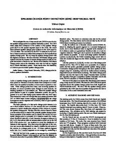
Modularity The algorithm is highly modular: any hazard H(t) ∈ [0, 1] can be plugged in. Likewise, any model that provides a posterior predictive, even multivariate ones, can be used for (r) p(xt |rt−1 , xt ). We have implemented BOCPD modules for changing Gaussian process regression, Bayesian linear regression, and Kernel Density Estimation. Caching Because predictions are usually made in an online fashion, and predictions under given (r) run lengths are made repeatedly, the predictive modules for p(xt |rt−1 , xt ) can usually be speed up using intelligent caching. Results Our method performs well on three real world data sets. The well log data is univariate while the others are multivariate. In all of the examples we use the three parameter logistic hazard, H(t) = hσ(at + b), to have a more flexible inter-arrival distribution than the geometric distribution implied by the constant hazard function. Well Log Data We applied our method to the well log data set for detecting changes in the rocks stratification, described in [4]. We used the logistic hazard and used a normal for the data in each regime, with changing mean and variance. After learning the parameters our method has a better predictive likelihood than [4]. We summarize our results in Table (1). Industry Portfolio Data We also tried a multivariate data set: the “30 industry portfolios” data set1 , which was also in the context of change point detection by [3]. The data consists of daily returns of 30 different industry specific portfolios from 1963 to 2009. The portfolios consist of NYSE, AMEX, and NASDAQ stocks from industries such as food, oil, telecoms, retail, etc. For financial returns the iid assumption within a regime is quite reasonable. However, the data is heavy tailed and our change point model assumes the data is normal within a regime. It is possible to justify the normality assumption with a change point model by claiming every heavy tail event is merely a change in variance. This will lead to very frequent change points. So, we transform the data set using the normal quantile function Φ−1 and t CDF with four degrees of freedom, x˜t := Φ−1 (t-cdf4 (xt )), to implicitly build the heavy tail assumption into the model. We could directly model the data using t distributions, but we would lose the tractability from conjugate priors. In Fig 1, we show that the change points found coincide with significant events with regard to the stock market the climax of the Internet bubble, the burst of the Internet bubble, and the 2004 presidential election. The methods used in [3] did not find any correspondence with historical events. Furthermore, this change point model has a better predictive likelihood of market returns than modeling it by iid t distributed (robust to heavy tail behavior); and much better than iid normal. This is noteworthy since treating market returns as random iid samples is generally a good model. The joint BOCPD performed better than the independent BOCPD, although with a large p-value. The joint BOCPD assumes change points effect the whole market while the independent model allows different parts of the market to have different change points. Although this is more flexible, the joint model can extract more information from the data as simultaneous changes in multiple time series is a strong indication of a change point. Changes points identified by the joint model tend be in between an AND/OR operation on the independent models. The results are shown in Table (1). Satellite Transmission Systems We also apply BOCPD to a satellite transmission systems data set using measurements such as current, voltage, and temperature from a high power amplifier (HPA). Sudden changes in any of these quantities can represent a change in system state or failure in a system component. Technicians managing such systems want to know when system changes occur. We omit the results for space limitations. Conclusion We have introduced a procedure to learn hyper-parameters in BOCPD, which can improve its performance. It makes change point detection much more robust as BOCPD can be sensitive to hand 1 The data can be found at http://mba.tuck.dartmouth.edu/pages/faculty/ken. french/Data_Library/det_30_ind_port.html
3
Dot−com bubble burst September 11 Asia crisis, Dot−com bubble
US presidential election Major rate cut
Northern Rock bank run Lehman collapse
Run Length (trading days)
50 100 150 200 250 300 350 400 450 1999
2000
2001
2002
2003
2004
2005
2006
2007
2008
Date (years)
Figure 1: Output of joint BOCPD run length distribution in 1998–2008. The color represents the CDF of the run length distribution, while the red line represents the median of the distribution. Areas of a quick transition from black (CDF of zero) to white (CDF of one) indicate a sharply peaked run length distribution. Many events of market impact create change points. Some of the other change points correspond to minor rallies or rate cuts but not a historical event.
Table 1: A summary of comparing the negative log predictive likelihoods (NLL) (nats/observation) on test data. We also include the 95% error bars on the NLL and the p-value that the joint model/learned hypers has a higher NLL using a one sided t-test. A reference method, the time independent model (TIM), treats the data as iid, normal for the well log and t for industry data. The TIM parameters are fit to the training set. Well Log: The learned hyper-parameter method was trained using the first 1000 points and tested on 3050 points. Industry: We test on the last 8455 points of the portfolio data, 3 July 1975–31 December 2008. The the methods were trained using the first 3000 points, 1 July 1963–2 July 1975. We compare running BOCPD independently on all 30 time series and using one joint BOCPD.
Method TIM fixed hypers learned hypers
Well Log NLL error bars 1.53 0.0449 0.313 0.0267 0.247 0.0293
p-value 0 5.96e-04 NA
Method TIM indep. joint
Industry Portfolios NLL error bars p-value 42.6 0.246 4.79e-74 39.64 0.217 0.271 39.54 0.213 NA
picked hyper-parameters. Online predictions and run length estimation can be done exactly and quickly. We have shown it can be successfully applied to multivariate and real world data sets. MATLAB code is available at http://mlg.eng.cam.ac.uk/rdturner/bocpd/.
References [1] D. X. Li, “On default correlation: A copula function approach,” Working paper 99-07, The RiskMetrics Group, 44 Wall St. New York, NY 10005, April 2000. [2] S. Jones, “The formula that felled wall st,” in Financial Times, April 2009. [3] X. Xuan and K. Murphy, “Modeling changing dependency structure in multivariate time series,” in Proceedings of the 24th International Conference on Machine Learning, 2007. [4] R. P. Adams and D. J. MacKay, “Bayesian online changepoint detection,” tech. rep., University of Cambridge, Cambridge, UK, 2007. arXiv:0710.3742v1 [stat.ML].
4