[8] M. Maimone, A. Johnson, Y. Cheng, R. Wilson, and. L. Matthies. Autonomous navigation results from the mars exploration rover (mer) mission. 2006. [9] Trey ...
ADAPTIVE SUBSAMPLING OF IMAGE SEQUENCES FOR REMOTE EXPLORATION ˜ 3 David R. Thompson1 , David Wettergreen2 , and Rebecca Castano 1
now at Jet Propulsion Laboratory, California Institute of Technology 2 Carnegie Mellon Robotics Institute 3 Jet Propulsion Laboratory, California Institute of Technology
ABSTRACT Planetary exploration robots currently collect science images at a very limited rate due to communications bandwidth constraints. Onboard image understanding can improve science return; the remote agent can collect many images and then select informative subsets for transmission at each communications opportunity. Often due to the inherent complexity of object recognition essential image features are hidden from the autonomous agent during subsampling. We present a method to select information-optimal summary subsets without detecting the content of interest directly. Instead, the remote agent leverages correlated proxy features that act as latent input dimensions in a Gaussian process model. We formulate selective image transmission as an active learning problem in which the agent chooses an observation set that maximizes information gain over the unknown image contents. Experiments in autonomous geologic site survey use texture-based image analysis to improve selective subsampling of rover navigation image sequences. Key words: Autonomous Science, Computer Vision, Active Learning, Gaussian Processees.
1.
Figure 1. The rover Z¨oe during autonomous traverse at the Amboy Lava Field. This portion of the lava field consists of two principal terrain types, basalt mounds and sediment, which are both visible in the background.
related image attributes that function as latent input dimensions in a Gaussian process model. We formulate representative subsampling as an active learning problem [7] in which the agent chooses an observation set that maximizes information gain with respect to the content of interest.
INTRODUCTION
Many planetary exploration scenarios involve an autonomous remote agent that images a spatially- or temporally-varying process [1, 2]. This work considers the task of summarizing image sequences to an operator using a small subset of collected data. The method is applicable whenever the images are too numerous to display [3] or when the remote agent can only transmit a small portion due to bandwidth constraints [4, 5]. In our approach the agent sends a subset of images that best represents the content of the complete dataset. However, the human operator may be interested in phenomena that the automatic system cannot detect reliably [6]. Due to this asymmetry, essential attributes of the data products are unknown during the subsampling procedure. Our method finds informative subsets without detecting the content of interest directly. Instead the remote agent leverages cor-
We consider the specific domain of science image sequences obtained during planetary exploration. This is a particularly suitable application: spacecraft must operate autonomously for long periods between communications opportunities and bandwidth may limit transmissions to a handful of data products [4]. Moreover, image sequences result from common spacecraft activities such as flybys, lander descent imagery, and rover navigation [8]. These sequences often contain many similar images, slow trends, and occasional moments of abrupt change. However, conventional periodic sampling methods return images at regular spatial or temporal intervals [9]. They ignore content redundancy and risk under-sampling the most important transient events. Exploration missions can benefit from onboard data analysis; the spacecraft can interpret the science content of collected data to identify the most informative images to
transmit. However, remote science favors phenomena at the limits of perceptibility and scientists will inevitably consider features of the data that are too abstract or subtle for automatic pattern recognition. Geologists analyzing Mars Exploration Rover imagery have considered sediment structure [10] and the morphology of rocks and outcrops [11]. These present significant pattern recognition challenges; reliable automatic feature detectors may not be feasible. This work describes field tests at Amboy Crater (Figure 1) in which automatic descriptor attributes suggest the most informative m frames in sequences of rover navigation imagery. Here texture-based image analysis improves selective subsampling during autonomous geologic site survey. Our method learns to infer changes in image geomorphology from these correlated texture descriptors without explicitly detecting the geologic features themselves.
to different image attributes. (
APPROACH
We represent a set of n collected images as A = {ai }ni=1 associated with corresponding attribute vectors X = {xi }ni=1 , xi ∈ IRD . Each attribute vector includes one or more independent variables, such as the temporal position, as well as numerical image descriptors produced by automatic analysis. For example, a position ti ∈ IR and an image descriptor di ∈ IR produce an augmented attribute vector xi = [ti , di ] ∈ IR2 . The dimension of xi is generally low, reflecting the fact that these summary attributes are far more compact than the original images. They generally require trivial bandwidth to transmit, so the agent can freely communicate the entire matrix X of attributes for the whole sequence. In addition to the attribute vector each image is associated with some science content, e.g. its actual semantic interpretation. For example, in our case study application of geomorphology the relevant content is the type of terrain appearing in the image. For simplicity we will treat science content as a scalar value so the sequence defines a vector s = {si }ni=1 with each element corresponding to the content of an individual image. Gaussian process regression [12, 13] models the science content with an underlying function of the attribute vectors f (x) : IRn 7→ IR. We define si = f (xi ) + N (0, σ 2 ) such that image contents are the underlying function perturbed by Gaussian-distributed noise. This formulation permits classifier or multiple-output Gaussian processes for more sophisticated representations, but we will limit these experiments to the case where science content is described by a single scalar label. This content is apparent to an operator viewing the image but invisible to the remote agent. We determine a prior distribution over possible content using a covariance matrix K with elements given by a covariance function Kij = κ(xi , xj ). We employ the common squared exponential covariance function [13] parameterized by θ = {ψ1 , ψ2 , w1 , . . . , wn }, where w are length scale hyperparameters corresponding
k=1
)
(1)
For a vector-valued f (X) (representing f (x) evaluated for multiple attribute vectors), we take the prior distribution to be a zero-mean multivariate Gaussian, f (X) ∼ N (0, K). Thus the prior over image content is also Gaussian-distributed: p(s | θ) = N (s | 0, K + σ 2 I)
(2)
Given a set of labeled training images with attributes XL and associated content sL , we wish to compute the posterior distribution over unknown contents s at locations X. We can do so by conditioning the joint Gaussian: p(s | sL , θ)
2.
d
1 X (xik − xjk )2 κ(xi , xj ) = ψ1 + ψ2 exp − 2 wk2
ˆ = N (s | µ ˆ, Σ)
(3)
The result is given by the standard Gaussian process prediction equations [13]: µ ˆ = κ(X, XL )T Q−1 sL (4) T −1 ˆ Σ = κ(X, X) − κ(X, XL ) Q κ(XL , X) (5) Q = κ(XL , XL ) + σ 2 I
(6)
Note that without training images, the prior covariance of s is simply the covariance given by κ(X, X). We formulate remote exploration as a three-part procedure. During an initial training phase experts label a set of training images AL with content sL . The agent explores the remote environment and collects a set of unlabeled images A, of which it can only communicate a small subset AO . The remainder AU refers to the untransmitted images that operators will never see: A = AO ∪ AU . The operators receive a transmission consisting of the subset AO along with all the image attributes X. They observe the true image contents sO and infer unobserved image contents sU . Figure 2 illustrates a graphical decomposition of the selective image return task. Each node is shaded to indicate whether the operator and/or explorer can observe its value. Note that our covariance function is stationary; covariance is independent of the two images’ absolute attribute values. This property means that hyperparameters θ can generalize across environments with similar covariance relationships. For practical purposes the training and test images are infinitely separated in space, so we define them to be independent given the covariance hyperparameters θ. By conditional independence,
and
P (sO | sL , sU , θ) P (sU | sL , sO , θ)
= P (sO | sU , θ) = P (sU | sO , θ)
(7) (8)
The agent tries to partition collected images into AU and AO in order to improve the reconstruction of sU . This is tantamount to an active learning or experimental design
Note that the hyperparameters and image attributes completely determine the elements of K. These are independent of the actual contents in s. This is true for any information gain metric based on a fixed stationary covariance matrix; image attributes alone define the best observations. An alternative experimental design criterion that meets this standard is the classic Maximum Entropy Sampling (MES) criterion [15].
Figure 2. Hand-labeled training values sL permit maximum-likelihood learning of the hyperparameters θ. XL are independent attributes (locations and proxy features) of the training set, and f (XL ) is the Gaussian process that produces training data. In a new test environment, observed values and hyperparameters define a prior Gaussian distribution over image contents. The training and test images influence each other only through the shared parameters Θ of the stationary covariance function. The explorer splits the test set into a returned (observed) portion sO that is revealed to scientists and an unobserved portion sU . problem. We choose images whose contents are maximally informative with respect to the remainder when “revealed” to operators during transmission. Our agent’s utility function is based on information gain - the mutual information criterion [13]. Guestrin et al. demonstrate desirable properties of the mutual information for choosing observation sites in Gaussian process models [2]. Our objective R(AO ) favors the size m subset AO which maximizes the mutual information I(sO ; sU ) between the contents of untransmitted images and the transmitted images. R(AO ) = I(sO ; sU ) for A = AU ∪ AO , |AO | = m (9) Correlations between image attributes and content let us choose AO adaptively, improving the objective without observing sU or sO directly. For Gaussian-distributed observations the mutual information is defined solely in terms of the covariance matrix. We separate the covariance matrix K into block diagonal form, with submatrices associated with the transmitted portion κ(XO , XO ) and the remainder κ(XU , XU ): � � κ(XO , XO ) ... (10) K = ... κ(XU , XU ) The mutual information of the returned images’ contents with respect to the unobserved images can be written in terms of differential entropies h or expressed using submatrix determinants [14]. Applying the equality from equation 8 yields: I(sU ; sO | sL , θ) (11) = h(sO | sL , θ) + h(sU | sL , θ) − h(s | sL , θ) (12) = h(sO | θ) + h(sU | θ) − h(s | θ) (13) 2πem |κ(XO , XO | 2πen−m |κ(XU , XU )| 1 (14) = log 2 2πen |κ(X, X)|
The labeled training images still play an important role in estimating θ. During the training phase, the agent learns covariance function parameters using classical gradient ascent of the likelihood p(sL |θ) or by Bayesian methods such as Markov Chain Monte Carlo simulation. Researchers have investigated similar ideas under the heading of hierarchical Bayesian hyperparameter learning or multi-task learning [16]. Our scenario differs in that the content is hidden, e.g. the agent never receives any direct observations from the test environment. At runtime the agent extracts relevant image descriptors using onboard analysis and uses the learned hyperparameters to compute a prior covariance matrix. This is sufficient to evaluate the objective of equation 14 for any transmitted subset. The following experiments use evidence maximization to produce a point estimate of θ. We then optimize the objective of equation 14 through the pairwise swapping algorithm of Shewry and Wynn [15]. The algorithm begins with a greedy initialization and then tries all possible substitutions of untransmitted images into the downlink subset, accepting any swaps that improve the objective. In our experiments this procedure always converged to a local minimum within 10 swaps. While this method produces good results in practice, the general problem of observation subselection is NP-complete [2] and one might still improve optimality through more expensive optimization strategies such as simulated annealing or the branch and bound method of Ko et. al [17]. Some examples illustrate image attributes’ influence on subsampling behavior. Consider the step function portrayed in Figure 3 (Top). This simulated environment consists of two flat homogeneous regions separated by a discontinuity. When the agent only has access to the the spatial dimension, our experimental design criterion seeks observations that fill the available space. This amounts to periodic sampling that ignores observations’ content. Figure 3 (Bottom) shows the covariance matrix and sampling behavior for this simple image return scheme. Black dots along the diagonal of the covariance matrix indicate the most informative subset of two images. In the topmost case, information-optimal data return reduces to even spatial coverage. This provides intuitive support for conventional image return strategies. If one assumes some degree of correlation between neighboring locations but has no other information about observations’ content then periodic sampling is information optimal according to Equation 9. Figure 4 shows a similar scenario with the Gaussian process trained on a two-dimensional input: one dimension
Input: budget m, hyperparameters θ, image products A, attributes X, AU = A, AO = {} Output: transmission subset AO while |AO | < m do a = argmaxa∈AU R(AO ∪ a) AU ← AU \ a AO ← AO ∪ a for aO ∈ AO do for a ∈ AU do A⋆O ← {AO \ aO } ∪ a A⋆U ← {AU ∪ aO } \ a if R(A⋆O ) > R(AO ) then AO ← A⋆O AU ← A⋆U return AO
Algorithm 1: Selective image transmission based on supervised learning of image contents.
corresponds to an observation’s physical position and another is a synthetic feature resulting from onboard pattern recognition. Here the blue dashed line represents the actual image content, while the black line represents the agent’s (noisy) image descriptor attributes computed automatically. The two lines represent different quantities so we offset them vertically to emphasize that their values are not to scale. However, in this domain, change in image content correlates with change in the descriptor. The labeled training images reveal this relationship; the length-scale hyperparameters and the resulting covariance matrix reflect this correlation. Finally, Figure 5 shows a Gaussian process with hyperparameters trained on image descriptors that closely match the true content labels. The resulting covariance structure reflects the discovered redundancy; one can observe the contents of the large, homogeneous portion of the input space with just a few measurements. Image content correlates strongly along this dimension and obviates the need for dense sampling. This is tantamount to a subsampling strategy that emphasizes diversity of data products rather than even physical spacing. The operators would see both the returned data products themselves and the noisy predictions in blue so they would be able to reconstruct the true environment with high accuracy. Thus existing heuristic sample return strategies from the exploration literature, such as spatially-periodic subsampling [9] and representative subsampling [4, 18], can be justified on information-theoretic grounds. These special cases simply make different assumptions about the noise in onboard image analysis and the spatio-temporal relationships in image contents. A model describing correlations between image attributes and science contents makes these assumptions explicit; one can learn the appropriate parameters directly from training images.
Figure 6. Covariance matrix for the Figure 7 traverse. 3.
FIELD TRIALS
This section evaluates the image sequence subsampling in an experimental analog of robotic planetary exploration. We consider a geologic site survey task in which operators map surface material visited during kilometerscale rover traverses. The base dataset consists of navigation image sequences from Amboy Crater, a lava flow located in the Mojave Desert, California (Figure 1). Our investigation focuses on the East end of the lava flow where the terrain consists of two principal types: basaltic lava platforms and areas of deposited sediment. The investigations aimed to characterize the geomorphology of basaltic platforms and identify the different densities of basalt at different locations along each rover traverse. Our rover platform is “Zo¨e,” an exploration rover developed at the Carnegie Mellon Robotics Institute for long range autonomous navigation [6, 19]. Zo¨e is approximately 2 meters in length and travels at up to 1m/s under solar power. Autonomous path planning using stereo terrain evaluation provides waypoint navigation and hazard avoidance. The stereo cameras produce a continuous stream of images with considerable overlap and redundant content. The goal of selective image return is to return the subset of navigation images that best describes the density of basalt along the rover path.
3.1.
Method
The rover performed an autonomous transect approximately 200-300 meters in length for each trial. It acquired navigation images at 2 meter intervals. We use 320 × 240 pixel navigation images with a 60-degree field of view directed at the surface directly in front of the rover. We selected a total of 7 trials for their superior lighting conditions: in particular, they lacked rover shadows which otherwise confuse the texture analysis. Of these, we reserved the first as a training set and tested system performance on the remaining 6 runs. Each traverse crossed several boundaries between sediment and basalt terrain.
Figure 3. Top: Image return based only the position attribute. The noisy step function appears above, and the associated covariance matrix below.
Figure 4. Optimal image return using position attribute and a noisy image content attribute. The additional input is a rough correlate of the true image label.
Figure 5. Inputs include position attribute and an accurate image descriptor. Here the Gaussian process model infers strong non-local correlations.
We produce ground-truth image content labels through manual inspection. The images show varying mixtures of two main terrain types: sediment composed of light material and basaltic lava characterized by fields of dark, dense rocks. We ascribe a value of −1.0 to images containing less than 50% basalt by pixel area, and 1.0 to those containing over 50% basalt. We made no attempt to express subtler distinctions using intermediate values although the model would certainly accomodate them. The Gaussian process used a 2-dimensional input space consisting of the physical imaging position along the traverse and a single scalar image texture attribute. We computed the texture attribute using textons extracted from the foreground half of the image [20]. Textons are pixel-level texture classifications generated in our case by convolving a training set of images with the Maximum Response 8 filter bank. This produces an 8-dimensional response vector for each pixel; responses are aggregated and clustered using k-means to form a set of 32 “universal” textons describing canonical texture categories. Different textons approximately capture the different classes of surface materials such as basalt and sediment.
Figure 8. Mean absolute reconstruction error. Error bars indicate 95% confidence intervals based on 6 traverses.
The proportions of each texton in the images form a 32dimensional image descriptor; we compress it to a single scalar value using Principal Component Analysis. For a novel image we perform the filter bank convolution and assign each individual pixel to its Euclidean-nearest texton. The resulting histogram of texton counts, projected into the basis learned from the training images, reflects the new image’s content according to the principal distinction in the training set.
3.2.
Results
Figure 7 shows the time series resulting from one of the test sequences. The blue dashed line indicates ground truth image content for the traverse. This correlates well with the image descriptor shown here by a black dotted line. Again, we offset the two lines vertically to emphasize that they represent different (but correlated) quantities. We reduce noise by smooth the image descriptor values using a secondary latent Gaussian process model to produce the second image attribute. Over time its distribution is approximately bimodal, reflecting the two distinct classes of surface material at the site. Figure 7 also shows the actual images from the optimal size-4 downlink. These constitute a representative sample of the principal terrain types from different areas of the traverse. The subset selection is aperiodic: selective return allocates a single image to the large homogeneous sediment patch in the first half of the traverse, and two closely-spaced images to the rapid transitions near the end. The associated covariance matrix appears in Figure 6. The environment exhibits fairly sharp discrete boundary transitions between basalt and sediment units. These transitions combined with a distance-decaying spatial correlation produce a covariance structure akin to a block diagonal matrix.
Figure 9. Reconstruction scores per traverse for all subset sizes. We provide adaptive and periodic sampling results for the six tests. Figure 8 shows reconstruction error for six trials of adaptive sampling compared to a periodic subsampling strategy that returns images at regular intervals and ignores image content. We produce a reconstruction by revealing the ground truth image contents for transmitted images. The resulting reconstruction consists of Maximum A Posteriori content values for all images based on a Gaussian process after conditioning on the revealed images’ contents. To ensure a fair comparison the input space of the reconstruction model incorporates the complete 2-dimensional image attribute even in the periodic cases where subselection ignores image content. This reflects scientists’ presumed ability to infer the image contents of other locations in the traverse based on all the available returned information. Figure 8 shows mean absolute errors for various subset sizes. The adaptive method utilizing the mutual information criterion significantly outperforms periodic image return for small values of m. Here an error value of 1.0 corresponds to an inference procedure that guesses either class with equal probability, while 0.0 is a perfect reconstruction. Figure 9 illustrates the per-traverse spread of reconstruction errors. For this environment reconstruc-
Figure 7. Example trial from the Amboy lava field dataset. Dots indicate images comprising the size 4 optimal downlink. tion error for adaptive sampling appears consistently better across traverses and more reliable across different subset sizes within a single traverse. Figures 11 - 12 provide some insight into typical subsampling behavior for three other traverses. Here again the horizontal axis shows the spatial dimension, and the solid black line indicates noisy observations with the texture feature on the vertical axis. The blue line (offset, not to scale) shows ground truth labels for each image. Circles and triangles indicate subsets of sizes 4 (circles), and 6 (triangles) returned by the algorithm for each of these image budgets. The adaptive method transmits representative samples from the principal terrain types as determined by both spatial proximity and difference in the image descriptors. Image return favors areas of high change like unit boundaries and ignores long homogeneous stretches like the sediment basin that dominates the first half of Figure 11. As the budget grows, the subsamle shifts to accomodate additional images while balancing diversity in content against spatial coverage.
4.
CONCLUSIONS
We have presented an approach for producing information-optimal summary subsets of temporal image sequences. Selective subsampling “encodes” the complete data set’s science content in a compressed representation: the returned images themselves and the attribute vectors of all other images. Our method is unique in that it explicitly accounts for data contents that are too subtle to detect directly using automatic pattern recognition. Instead we extract correlated descriptor attributes that are simple to detect. An active learning criterion indicates those observations which are most informative with respect to the underlying science content. This permits optimal summary of image sequences that respects both spatiotemporal correlations and the learned fidelity of the onboard pattern recognition.
ACKNOWLEDGMENTS We acknowledge the vital help and support of Francisco Calder´on, Dom Jonak, and James Teza. Thanks are also due advice and counsel from Jeff Schneider and Reid Simmons from the Robotics Institute, Steve Chien of JPL, and Phil Christiensen, Ron Greeley and Shelby Cave of Arizona State University. The work was carried out at Carnegie Mellon University. It was supported by a JPL Strategic University Partnership Grant. Data collection, and the Amboy expedition, was facilitated by the NASA ASTEP project NNG0-4GB66G ”Science on the Fly.” This text Copyright 2009, Jet Propulsion Laboratory, California Institute of Technology. All Rights Reserved. U.S. Government Support Acknowledged.
REFERENCES [1] A. Singh, A. Krause, C. Guestrin, W. Kaiser, and M. Batlin. Efficient Planning of Informative Paths for Multiple Robots. In IJCAI, 2007. [2] C. Guestrin, A. Krause, and A. Singh. Near-optimal Sensor Placements in Gaussian Processes. School of Computer Science, Carnegie Mellon University, 2005. [3] Santhana Krishamachari and Mohamed AbdelMottaleb. Image browsing using hierarchical clustering. The Fourth IEEE Symposium on Computers and Communications, page 301, 1999. [4] Rebecca Casta˜no, Robert C. Anderson, Tara Estlin, Dennis DeCoste, Forest Fisher, Daniel Gains, Dominic Mazzoni, and Michele Judd. Rover Traverse Science for Increased Mission Science Return. In IEEE Aerospace, March 2005. [5] V. C. Gulick, R. L. Morris, M. A. Ruzon, and T. L. Roush. Autonomous Image Analysis During the 1999 Marsokhod Rover Field Test. J. Geophysical Research, 106(E4):7745–7764, 2001. [6] Thompson, D. R. and F. Calder´on P. and D. Wettergreen. Intelligent Maps for Autonomous KilometerScale Science Survey. 2008.
Figure 10. Selected subsets for the second experimental traverse, shown here as time series plot of ground truth (blue dashed line) and the image texture attribute (black solid line). The algorithm favors images 45 − 85 that contain the most diversity of content. Results are shown for a strict “image budget” of size 4 and a more lenient budget of size 6.
Figure 11. Traverse 3 results showing returned subsets for two different image budgets.
Figure 12. Traverse 4 results showing returned subsets for two different image budgets.
[7] D. MacKay. Information-Based Objective Functions for Active Data Selection. Neural Computation, 4(4):590–604, 1992. [8] M. Maimone, A. Johnson, Y. Cheng, R. Wilson, and L. Matthies. Autonomous navigation results from the mars exploration rover (mer) mission. 2006. [9] Trey Smith, David R Thompson, Shmuel Weinstein, and David Wettergreen. Autonomous rover detection and response applied to the search for life via chlorophyll fluorescence in the atacama desert. March 2006. [10] N. A. Cabrol, J. D. Farmer, E. A. Grin, L. Richter, L. Soderblom, R. Li, K. Herkenhoff, G. A. Landis, and R. E. Arvidson. Aqueous processes at Gusev crater inferred from physical properties of rocks and soils along the Spirit traverse. Journal of Geophysics Research, 111:E02S20, 2006. [11] SW Squyres, JP Grotzinger, RE Arvidson, JF Bell, W. Calvin, PR Christensen, BC Clark, JA Crisp, WH Farrand, KE Herkenhoff, et al. In Situ Evidence for an Ancient Aqueous Environment at Meridiani Planum, Mars. Science, 306(5702):1709–1714, 2004. [12] C.K.I. Williams and C.E. Rasmussen. Gaussian Processes for Regression. Advances in Neural Information Processing Systems, 8:514–520, 1996. [13] David C. J. MacKay. Information Theory, Inference, and Learning Algorithms. Cambridge University Press, Cambridge, UK, 2003. [14] Thomas M. Cover and Joy A. Thomas. Wiley and Sons, New York, 1991. [15] M.C. Shewry and H.P. Wynn. Maximum Entropy Sampling. J. Applied Statistics, 14(2), 1987. [16] Anton Schwaighofer, Volker Tresp, and Kai Yu. Learning Gaussian Process Kernels via Hierarchical Bayes. Advances in Neural Information Processing Systems, 2004. [17] C.W. Ko, J. Lee, and M. Queyranne. An Exact Algorithm for Maximum Entropy Sampling. Operations Research, 43(4):684–691, 1995. [18] Trey Smith, Scott Niekum, David R Thompson, and David Wettergreen. Concepts for science autonomy during robotic traverse and survey. March 2005. [19] N. A. Cabrol et. al. Life in the Atacama: Searching for Life with Rovers. Journal of Geophysics Research, 112:G04S02, 2007. [20] M. Varma and A. Zisserman. A Statistical Approach to Texture Classification from Single Images. In International Journal of Computer Vision: Special Issue on Texture Analysis and Synthesis, volume 62:12, pages 61–81, 2005.