Adaptive System Identification Using Time-Varying Fourier Transform

ADAPTIVE SYSTEM IDENTIFICATION USING TIME-VARYING FOURIER TRANSFORM Hadas Benisty, Yekutiel Avargel and Israel Cohen Department of Electrical Engineering, Technion - Israel Institute of Technology Technion City, Haifa 32000, Israel {hadasbe@tx, kutiav@tx, icohen@ee}.technion.ac.il

Abstract In this paper, we introduce a time-varying shorttime Fourier transform (TV-STFT) for representing discrete signals. We derive an explicit condition for perfect reconstruction using time-varying analysis and synthesis windows. Based on the derived representation, we propose an adaptive algorithm that controls the length of the analysis window to achieve a lower mean-square error (MSE) at each iteration. When compared to the conventional multiplicative transfer function approach with a fixed length analysis window, the resulting algorithm achieves faster convergence without compromising for higher steady state MSE. Experimental results demonstrate the effectiveness of the proposed approach.

is derived, and a perfect reconstruction is achieved by enforcing a generalized form of the completeness condition. Based on the MTF approximation, an adaptive scheme for system identification, which utilizes the dynamic nature of the TV-STFT domain, is presented. Using a time-varying window length, the resulting algorithm achieves a relatively low steady state error without degrading its convergence rate. This paper is organized as follows. In Section 2, the TV-STFT and TV-ISTFT are defined, and a perfect reconstruction condition is obtained. In Section 3, an adaptive scheme for system identification is presented in the TV-STFT domain. In Section 4, experimental results demonstrate the effectiveness of the proposed approach.

2. Time-Varying STFT 1. Introduction The STFT of a signal System identification in the short-time Fourier transform (STFT) domain of linear time-invariant (LTI) systems is widely used in speech processing applications [1]-[6]. System identification in the STFT domain generally requires crossband filters between the subbands [4]. Nonetheless, when the STFT’s analysis window is long and smooth in comparison to the system’s impulse response, a single multiplicative term can be employed in each frequency bin. This approach is generally referred to as the multiplicative transfer function (MTF) approximation [6]. Since in real-world applications, the system to be identified is time-varying, adaptive estimation algorithms are required, using a finite amount of samples. In order to achieve a more accurate approximation and low steady-state error of the MTF approach, the analysis window should be as long and smooth as possible. However, a long window yields slower convergence than a shorter one. As a consequence, when choosing the analysis window length this trade-off has to be considered. In this paper, a time-varying STFT (TV-STFT) is defined using a time-varying window length. In addition, a time-varying inverse STFT (TV-ISTFT)

x p ,k =

is defined by [7]:

∞

∑ x(m)ψ

m =−∞

N

(m − pL)e

−j

2π k ( m − pL ) N

(1)

is an analysis window of length , where is the decimation factor, is the frame index and is the frequency-bin index. The ISTFT of , can be computed using the well known overlap and add formulation: 2π j k ( n − pL ) 1 ∞ N −1 (2) ISTFT { x p , k } = ∑ ∑ x p, kψ N (n − pL)e N N

p =−∞ k = 0

where is a synthesis window of length . Substituting (1) into (2) and enforcing perfect reconstruction of leads to the completeness condition [7]: ∞

∑ψ

N

( n − pL )ψ N ( n − pL ) = 1

∀n . (3)

p =−∞

Let us define a time-varying STFT (TV-STFT) of by:

 xt ,k =

∞

∑ x(m)ψ

m =−∞

N (t )

( m − t )e

−j

2π k ( m −t ) N (t )

(4)

where , is a time-varying analysis window, whose length is a piece-wise constant function: N (t ) = Nν tν −1 < t ≤ tν ν = 1, 2,.., V (5) and is the number of discontinuity points. denote a time varying decimation factor such Let that a fixed overlap is preserved: Nν Lν = const ∀ν . (6) The windows are centered at the time instants Γ defined by: Γ = {t t = tν −1 + rLν , tν −1 ≤ t < tν (7) t0 = −∞ , 0 ≤ r ≤ ( tν − tν −1 ) / Lν } .

3 interlaced 512.

which 75% overlap leads to windows around the transition point

(a) 200

400

512 600

800

1000

200

400

512 600

800

1,000

200

400

512 600

800

1000

(b)

(c)

Similarly to (2), the TV-ISTFT can be expreseed as:  TV − ISTFT { xt , k } =

N ( t ) −1

1

∑∑ N (t ) t ∈Γ

2π

j k ( n −t )  N t xt , kψ N ( t ) ( n − t )e ( ) .

(8)

k =0

Finally, substituting (4) into (8) and enforcing perfect reconstruction, yields the generalized form of the completeness condition:

∑ψ t∈Γ

N ( t ) ( n − t )ψ N ( t ) ( n − t )



= 1 ∀n .

(9)

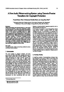
In order to demonstrate the structure of the analysis and synthesis windowing process, a simple case is presented, in which the analysis-window length is varied once: ⎧ N , for t < t1 , N (t ) = ⎨ 1 . (10) ⎩ N 2 , for t ≥ t1 The decimation factor is chosen so that the overlap between consecutive windows is retained, i.e., ⎧ L , for t < t1 , N N L (t ) = ⎨ 1 where 1 = 2 , (11) L1 L2 ⎩ L2 , for t ≥ t1 , and the analysis windows centers are: Γ = {t t = rL1 r ≤ t1 / L1 (12) or t = t1 + rL2 r > 0} . Note that the continuity of the window functions should be preserved when switching from . Then, since the number of windows to having non-zero values at the transition point is: ⎢⎡ N ⎤ ⎥ M = 2 ⎢ ⎢ 1 ⎥ − 1⎥ + 1, (13) ⎢⎣ ⎣ L1 ⎦ ⎥⎦ the continuity can be preserved by interlacing and : ⎧⎪ψ N ( n − t ) n < t1 ψ N1 → N 2 ( n − t ) = ⎨ 1 ⎪⎩ψ N 2 ( n − t ) n ≥ t1 (14) t1 − ⎣⎢ M / 2 ⎦⎥ L1 ≤ t ≤ t1 + ⎣⎢ M / 2 ⎦⎥ L2 . /2 , the windowing Specifically, for , , and for process is emploid using /2 , the windowing process will continue , . A simple example for this using windowing process is demonstrated in Figure 1, in

Figure 1. Time invariant windowing using a Hamming window (a) N = 128, L = 32 ; (b) N = 384, L = 96 ; (c) a time varying windowing process switching from N1 = 128, L1 = 32 (blue) to

N 2 = 384, L2 = 96 (black), at the transient point t1 = 512 using three interlaced windows (red dot).

The synthesis windows should sustain the generalized form of the completeness condition (equation (9)):

∑ψ t∈Γ

∑ψ t∈Γ

N1

( n − t )ψ N ( n − t ) = 1 1

n < t1 (15)

N2

( n − t )ψ N ( n − t ) = 1 2

n ≥ t1

, Recall that the analysis windows and their synthesis matches , satisfy (3). Since equation (3) holds for all , it also holds particularly for , which means that and sustain equation (9) in this time interval, so can be used as a synthesis window for . A similar claim can be made and , for . regarding Altogether, the windowing process of the TV-ISTFT divides the time domain into three parts: before, during and after the transition, that is, ψN( t ) ( n −t ) =

⎧ ψN ( n − t ) t < t1 − ⎢⎣M / 2⎥⎦ L1 (16) 1 ⎪⎪ = ⎨ψN1→N2 ( n −t ) t1 − ⎣⎢M / 2⎦⎥ L1 ≤ t ≤ t1 + ⎣⎢M / 2⎦⎥ L2 ⎪ t > t1 + ⎣⎢M / 2⎦⎥ L2 ⎪⎩ ψN2 ( n −t )

where

⎧⎪ψ N ( n − t ) n < t1 ψ N1 → N 2 ( n − t ) = ⎨ 1 . (17) ⎪⎩ψ N 2 ( n − t ) n ≥ t1

This formulation can be extended for any countable number of variation points, as long as the interlacing structure of the analysis and synthesis

windows is preserved. That is, at the non-transient /2 /2 ) frames (i.e., the TV-STFT and its inverse are computed using , , . At each transition point , interlaced windows [see (13)] should be used to switch from to . The following frames should be analyzed and synthesized using , , , up to the next transition point.

system using the normalized least-mean-square (NLMS) algorithm is identical to the one described in [5], using the appropriate window lengths and decimation factors. Denote: and ℓ , the NLMS equations are: ℓ  xt∗A , k ˆh Nν (t ) = hˆ Nν (t ) + μ e k k A +1 A tA , k  2 xtA ,k ˆ     N et , k = yt , k − d t , k = yt , k − xt , k ⋅ hˆk ν (tA ) A

3. Adaptive System Identification Using TV-STFT In this section we consider the problem of system identification using the previously defined TV-STFT. Let and be the input and output of an unknown LTI system, represented by its impulse response , with additive noise , i.e., y (n) = x (n) ∗ h (n) + ξ (n) = (18) = d (n) + ξ (n) The goal of system identification schemes is to based on samples of the input and estimate output signals. In many practical cases (such as [4][6]), this estimation is performed adaptively in the STFT domain to achieve both fast convergence and low computational cost. Applying the STFT on (18) produces: (19) y p ,k = d p ,k + ξ p ,k is much Assuming that the analysis window longer and smoother in comparison to the impulse , the MTF approximation can be responce applied [6]:

d p , k ≈ x p , k ⋅ hk(

N)

(20)

hk( N ) 

∑ h ( m)e

2π − j km N

A

A

(21)

m =−∞

The effect of the analysis window length on the estimation error was explored in [6], and a trade-off between the convergence rate and the steady-state value of the estimation error was presented. In order to avoid this trade-off, the TV-STFT can be employed. Specifically, at the beginning, a short window should be used in order to achieve fast convergence. Then, as the adaptation process proceeds, the algorithm should gradually increase the window length to produce a lower steady state MSE. Using the TV-STFT with the windowing process defined in (5)-(7) and the MTF approximation, (18) becomes:      N t ytA ,k = dtA ,k + ξtA , k ≈ xtA ,k ⋅ hk ( A ) + ξtA , k (22) Γ sorted in an where ℓ are the time instants ascending order so ℓ ℓ ℓ . At the nontransient frames, the adaptive estimation of the

(23)

A

tν −1 + ⎣⎢ M / 2 ⎦⎥ Lν < tA < tν − ⎣⎢ M / 2 ⎦⎥ Lν

is evaluated During the transient frames, using interlaced windows defined in equation (14), which means that its frequency–bins are not evenly spaced: (24) hkN(tA ) ( tA ) =

2π − j km ⎧ ∞ N N 0 ≤ k ≤ tν − tl + ν ⎪ ∑ h(m)e ν 2 ⎪ m=−∞ =⎨ 2π ∞ −j km ⎛ N ⎞ N N + Nν +1 ⎪ h(m)e Nν +1 tν − tA + ν < k < ν + tν − tA ⎜1− ν +1 ⎟ ⎪m∑ 2 2 Nν ⎠ ⎝ ⎩ =−∞ tν − ⎢⎣M / 2⎥⎦ Lν ≤ tA ≤ tν + ⎣⎢M / 2⎦⎥ Lν +1

Equation (23) cannot be used directly in these frames, since the frequency-bins resolution and the amount of estimated system coefficients do not match. In order to resolve this problem while preserving the continuity of the system identification process, the coefficients related to mismatched frequency-bins should be adjusted before forwarded to the next frame. The estimated impulse response can be obtained by: t (25) hˆ( A ) ( n ) = IDFTNν hkNν ( tA ) .

{

}

Switching to the next frequency–bins resolution is order DFT: performed by employing

{

}

N t t hk ( A+1 ) ( tA ) = DFTNν +1 hˆ( A ) ( n ) .

where ∞

A

(26)

To conclude, the required modification by the adaptive process is back and forward DFT according to the current and next window lengths. This adjustment ensures the continuity of the system identification process.

4. Experimental Results In this section, two simulations are presented. The first one uses white Gaussian noise as input in order to validate the analysis described above. The second simulation shows the applicability to acoustic echo cancellation by using a speech signal. Hamming window was taken as the analysis window with 50% overlap, and the synthesis window was its bi-orthogonal window. The noise is white, zero mean, and Gaussian with signal SNR of 30dB:

4.1. White Gaussian Noise

64 128 512 1024 TV-STFT

0

-5 Normalized Error

⎛σ 2 ⎞ SNR = 30dB = 10 log ⎜ x2 ⎟ (27) ⎜σ ⎟ ⎝ ξ ⎠ is the variance of the input signal , where . and is the variance of the noise signal The system’s impulse response was modeled as a multiplied by an white Gaussian noise exponential decay: h(n) = w(n) β (n)e−α n (28) And was taken as a rectangular window: ⎧1 0 ≤ n < N h w(n) = ⎨ (29) ⎩0 otherwise The decay exponent that was used: 0.03. The decimation factor was taken so a fixed overlap of 50% was sustained.

-10

-15

-20

0.2

0.4

0.6

0.8

1 Samples

1.2

1.4

1.6

1.8

2 4

x 10

Figure 3. Normalized MSE curves using fixed window lengths (64, 128, 512, 1024 samples), and TV-STFT. The impulse response was changed after 9200 samples 5

(

)

ˆ is the TV-ISTFT of dt ,k .

where

1200

1000

Window Length

800

600

400

200

0

0

0.2

0.4

0.6

0.8

1 Samples

1.2

1.4

-5

-10

-15

-20

-25

The mean was taken over 500 uncorrelated experiments. The impulse response was 16 samples long and was changed when convergence has been achieved – after 9,200 samples. Figure 2 shows the that was used by the window lengths function TV-STFT simulation. The shorter windows were used both at the beginning of the estimation and when the impulse response was changed. Figure 3 shows the normalized error for various window lengths using the conventional STFT and the TVSTFT. A smoothed version of these curves is presented in Figure 4.

1.6

1.8

2 4

x 10

Figure 2. Window length function N(n) used for the TV-STFT in the white Gaussian noise simulation.

64 128 512 1024 TV-STFT

0

Normalized Error

The input signal was taken as white, zero mean, unit variance Gaussian noise, uncorrelated . The performance of the system with identification was evaluated during 24,000 samples using the normalized mean square error (MSE) in the time domain: 2 E ⎡ d (n) − dˆ (n) ⎤ ⎢⎣ ⎥⎦ ε ( n) = (30) 2 E ⎡⎣ d (n) ⎤⎦

0

0.2

0.4

0.6

0.8

1 Samples

1.2

1.4

1.6

1.8

2 4

x 10

Figure 4. Smoothed (using Hamming window) noramlized MSE curves using fixed window lengths (64, 128, 512, 1024 samples), and TV_STFT. The implulse response was changed after 9200 samples.

Two methods for updating the estimated system coefficients at the transient frame were compared: One using IDFT and zero padded DFT as described above, and the second - by using cubic interpolation. Since both methods produced very similar results, the cubic interpolation was chosen in order to ease the complexity load. The trade-off between the convergence rate and the steady-state value is well demonstrated: the shortest window (64 samples) converges very quickly, but to a relatively high value. The longest window (1024 samples) achieves the lowest steadystate value, but with a very long convergence duration. This attribute is shown both at the beginning of the estimation and when the impulse response is changed. It is clear that the error obtained by the TV-STFT produced the lowest error during the whole simulation. Performing STFT and ISTFT is equivalent to using analysis and synthesis filter bank [7]. The output of

a synthesis filter bank is generally cyclo-stationary [8], so this is the reason for the periodic nature of the estimation error in Figure 3. In practical applications, there is no averaging over the estimation error, so this phenomenon is not disturbing.

4.2. Acoustic Echo-Cancellation In this simulation a practical usage for system identification using TV-STFT is demonstrated. Acoustic echo cancellation (AEC) can be modeled is the farusing equation (18): the input signal end signal coming out of a loudspeaker. The echo path of the room, from the loudspeaker to an . is an adjacent microphone, is modeled by additive white Gaussian noise, and the output signal is the recording microphone signal. In the simulation, the input signal was a speech signal sampled at 16kHz during 4 seconds. A 64 samples long impulse response was changed after 2 seconds. 1100 1000 900

Window Length

800 700 600 500 400 300 200 100

0

0.5

1

1.5

2 time [sec]

2.5

3

3.5

4

Figure 5. Window length function N(n) used for the TV-STFT in the AEC simulation

Figure 6 (a)-(b) shows the far-end speaker and the microphone signal respectively. The error signals Figure 6 (c)-(f) were calculated by applying TVISTFT on the error signals obtained by (23). A fixed window length of 128, 512, 1024 samples was used in Figure 6 (c)-(e) respectively. The TV-STFT was used in Figure 6 (f) with window length function as depicted in Figure 2. The fixed window estimation error suffers the same trade-off as before, whereas the TV-STFT achieves low error all through the estimation process.

5. Conclusions A time-varying STFT (TV-STFT) was introduced using a time-varying window length, and its inverse transform was calculated. A perfect reconstruction condition was explored and formalized. An adaptive scheme for system identification utilizing the dynamic nature of the TV-STFT domain was presented. Performing adaptive system identification using conventional STFT leads to a trade-off between the convergence rate and steady state value of the estimation error. Using a time varying window function resolves this trade-off and produces lower estimation error, and faster convergence rate. Experimental results confirmed that the TV-STFT approach outperforms the conventional STFT approach. Further work can be done concerning the time varying window function. In particular, derivation of the optimal values and the transition points online while considering the current stage of the estimation process and the instantaneous SNR conditions.

6. References

Amplitude

(a)

(b) (c) (d) (e) (f) 0

0.5

1

1.5

2 Time[sec]

2.5

3

3.5

Figure 6: Speech waveforms and error signals. The impulse response was changed after 2secs. (a) Far-end Signal; (b) near-end signal; (c)-(e) error signals for N=128, N=512, N=1024 respectively; (f) TV-ISTFT using N=[128 512 1024] starting at t=0secs and t=2secs.

4

[1] C. Faller and J. Chen, “Suppressing Acoustic Echo in a Spectral Envelope Space”, IEEE Trans. Speech, Audio Process., vol. 13. No. 5, pp. 1048-1062, Sep. 2005. [2] I. Cohen, “Relative transfer function identification using speech signals”, IEEE Trans. Speech Audio Process. (Special Issue on Multichannel Signal Processing for Audio and Acoustics Applications), vol. 12, no. 5, pp. 451459, Sep. 2004. [3] I. Cohen, “Identification of Speech Source Coupling Between Sensors in Reverberant Noisy Environments,” IEEE Signal Process. Lett., vol. 11, no. 7, pp. 613-616, Jul. 2007. [4] Y. Avargel and I. Cohen, “System Identification in the Short-Time Fourier Transform Domain With Crossband Filtering,” IEEE Trans. Audio, Speech, Lang. Process., vol. 15, no. 4, pp. 13051319, Apr. 2007.

[5] Y. Avargel and I. Cohen, “Adaptive system identification in the short-time Fourier transform domain using cross-multiplicative transfer function approximation,” IEEE Trans. Audio, Speech, Lang. Process., vol. 16, no. 1, pp. 162173, Jan 2008. [6] Y. Avargel and I. Cohen, “On multiplicative transfer function approximation in the short-time Fourier transform domain,” IEEE Signal Process. Lett., vol. 14, no. 5, pp. 337-340, May 2007. [7] M. R. Portnoff, “Time-frequency representation of digital signals and systems based on shorttime Fourier analysis,” IEEE Trans. Signal Processing, vol. 28, no. 2, pp. 55–69, Feb. 1980. [8] Ohno and H. Sakai, "Optimization of' filter banks using cyclostationary spectral analysis," IEEE Trans. Signal Process., vol. 44, no. 11, pp. 2718-2725, Nov. 1996.