Adaptive Thresholding Based Cell Segmentation for. Cell-Destruction Activity Verification. Praveen Sankaran and Vijayan K Asari. Department of Electrical and ...
Adaptive Thresholding Based Cell Segmentation for Cell-Destruction Activity Verification Praveen Sankaran and Vijayan K Asari Department of Electrical and Computer Engineering Old Dominion University, Norfolk, Virginia {psankara, vasari}@odu.edu Abstract An adaptive thresholding method used to distinguish cell boundaries in a given image is presented in this paper. A preprocessing step involves low pass filtering of the image to remove high frequency noise seen in the image. This image is now adaptively thresholded to create a binary image. The bright regions are further analyzed based on their geometrical descriptors such as area and form factor to classify them as cell or non-cell regions. Two sets of images, pulsed and non-pulsed, are available, which can be compared to determine the efficiency of the pulsing. Results for automatic segmentation are compared with those of manually obtained values to determine its efficiency.
1. Introduction Electrical pulses penetrate into the interior of the tumor cells and cause the nuclei to rapidly shrink and cause the tumor blood flow to stop [1]. Microscopic images taken before and after pulsing shows change in fluorescence of the cells which can be used to measure the effectiveness of the pulsing applied. To get a quantitative measure for this change, intensity of pixels in both the images have to be compared. Manually marking out the boundaries of each cell in an image is a very tedious job. Also, the accuracy of the whole procedure is now dependent on how accurate the cell regions were marked. This necessitates an automatic cell segmentation technique to extract cell regions from the background image. The adaptive technique [2] developed for computation of the threshold depends only on the spatial characteristics of the image. Previous work [3] has shown that this method does a better job at finding an optimal thresholding point when compared to other adaptive methods like the Otsu method. This is important as pre-fixing a value is inappropriate since
35th Applied Imagery and Pattern Recognition Workshop (AIPR'06) 0-7695-2739-6/06 $20.00 © 2006
the intensity values of “before” and “pulsed” images are found to be varying drastically. The raw images of “before” and “pulsed” images were provided by the Center for Bio-electrics at Old Dominion University. These images were low-pass filtered as a pre-processing step for noise removal and then adaptively thresholded. The edges were linked on the thresholded image to obtain cell boundaries. Once the boundary locations are obtained, rest of the processing is done on the original images with these boundary values. Fluorescence intensity measurements in “before” and “pulsed” picture with same mask-size at comparable positions are taken. This forms the basis for determining the efficiency of the pulsed energy method. The darker the “pulsed” image is, the better it is. A mask is run through each pixel inside the cell boundary. Measurements of mean, minimum and maximum values for “before” and “pulsed” picture are taken inside the region covered by the mask. Values obtained for the “before” and “pulsed” images are compared. This procedure is repeated for all cells in the image. The accuracy of the method is verified by comparing the results of the automated method with those obtained by manual method. The paper is organized in the following way. Section 2 gives a simple segmentation method without any preprocessing. Section 3 illustrates the noise removal procedure. Section 4 describes the adaptive thresholding. Section 5 shows cell classification based on cell area and form factor. Section 6 describes a procedure to verify the cell destruction activity and compares the results of the two methods.
2. Simple Segmentation A simple edge based thresholding is carried out on the given images. The threshold value is set as a percentage of the maximum pixel value found in the image. The need for preprocessing is justified by the poor results given by the fixed threshold segmentation
method. Figure 1 shows the result of the current method on a cell image. The noise in the image causes a very poor segmentation result. Hence, a preprocessing step to remove high frequency noise from the image is included.
Figure 2: Segmented image with nonlinear filter based preprocessing
4. Adaptive Thresholding Figure 1a: Original cell image
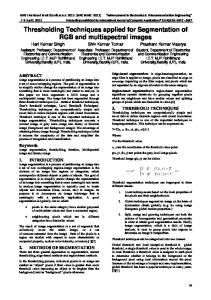
A fixed threshold value does not work well for a cell image due to illumination variation from one image to the other. This problem is illustrated in figure 3a where, a fixed percentage of the maximum value is used to threshold two different images in the database. Figure 3b shows the differences in the output image due to a separate percentage. This shows that there is no way we can arrive at predefined values that works well for all images.
Figure 1b: Segmented image with a fixed threshold
Figure 3a: Images with threshold factor = 0.1
3. Preprocessing: Noise Removal The strong noise presence in a cell image requires that we use a low pass filter. But, the main process requires that the edges of the cells do not get blurred too much due to filtering. Hence nonlinear median filtering [4] is used to remove the unwanted noise. This was found to provide better result after segmentation when compared with low-pass filters such as a Gaussian kernel. Figure 2 shows the result of segmentation after noise removal for the image shown in figure 1a. The filtered image shows better demarcation between the cells.
35th Applied Imagery and Pattern Recognition Workshop (AIPR'06) 0-7695-2739-6/06 $20.00 © 2006
Figure 3b: Images with threshold factor = 0.3 An adaptive technique is developed for computation of the threshold that depends only on the spatial characteristics of the image. The segmentation procedure begins with the computation of an optimum threshold to distinguish the darker regions in the image. It is an automatic thresholding algorithm that would work under all lighting conditions where pre-fixing of
threshold value is considered ineffective. The proposed algorithm is described as follows: Given an image of size M × N pixels consisting L gray levels. The spatial location of a pixel (x, y) would correspond to a gray level g(x, y). The image function as a mapping can be defined as: g:M×N→P (1) A smoothed image can be generated by passing the image through a smoothing filter S of window size s × s. The smoothed image is represented as:
g '( x, y ) =
1 s2
∑
g ( x + k , y + 1) ∀( x, y )∈ M × N (2)
( k ,1)∈S
The thresholding method is based on Otsu’s method [5], which follows the discriminant analysis. This partitions the L gray levels in the image into two classes P0 = {0, 1, 2…,t} and P1 = { t +1, t +2…L - 1} at gray level t. The total variance ( σ T2 ) and the between-class variance ( σ 2B ) are computed. The normalized between-class variance ( σ B2 / σ T2 ) is maximized and the optimum threshold t* is the gray level corresponding to the maximum normalized between-class variance.
σ 2 t * = arg max B2 σ T
t
n
t
(3)
n
σ B2 = ∑ i 1 − ∑ i ( µ1 − µ2 ) N N i =0
2
L −1
σ T2 = ∑ ( i − µT ) i =0
2
ni N
(4)
(5)
where
i × ni N i=0
L −1
µT = ∑
(6)
µ T is the total mean of the original image, N is the total number of pixels present in the image and n i is the number of pixels at the i th gray level, i × ni N µo = i =0t ni ∑ i =0 N t
∑
i × ni i =0 N t n 1− ∑ i i =0 N t
µ1 =
µT − ∑
(7)
µ 0 is the class mean for P0, µ1 is the class mean for P1 and µT is the total mean for the initial image. The cumulative limiting factor is calculated for each progressive image as:
35th Applied Imagery and Pattern Recognition Workshop (AIPR'06) 0-7695-2739-6/06 $20.00 © 2006
σ B2 (∆) for ∆ ≥1 σ T2
(8)
From here we can follow two directions in that we can have two different criteria for stopping the iterations. In the first case, the iteration is stopped when the cumulative factor meets the condition in equation 9.
CLF (∆) = α
µT σ T2
(9)
The problem here is that the factor α has to be obtained by training the image set. The value of α depends on the camera used, reflection characteristics of the object and the lighting environment of the images. This poses a challenge in the images under consideration. The second case tries to compute the limiting factor from the spatial characteristics of the image thus removing the dependence on the factor α. The image has a spatial distribution that is random in nature. The measures of randomness [6, 7] provide a number of ways for the analysis of spatial data. It is assumed in spatial data analysis that the observations follow a Poisson distribution, whose characteristic feature is that its mean is equal to its variance. A natural test for the Poisson distribution is the ratio of the sample mean, which is called relative variance [8, 9] which can be computed as:
Vr =
i =0
CLF (∆ ) =
σ T2 µT
(10)
It has been observed that in all the experiments that were conducted the relative variance was greater than one. The test for the frequency distribution corresponds to a negative binomial distribution in the test images. Hence, the separability factor for obtaining the optimum threshold is related to the relative variance and is defined as the square root of the inverse of it. That is,
SF =
µT σ T2
(11)
The cumulative limiting factor is compared with the separability factor and the process of recursive thresholding is stopped when the condition CLF ( ∆ ) < SF
(12)
is satisfied. The separability factor thus helps in stopping the algorithm at a point where the pixels are present as dense clusters, which is a characteristic of the negative binomial distribution. This clustered nature of the pixels causes the object region to be prominent with the background completely thresholded. The concept is shown in figure 4.
where, S is the area and P is the perimeter. Figure 6 shows the result for this step.
Figure 6: Corrected image
6. Image Comparison for Validation Figure 4: Illustration of the concept of APT
Figure 5: Result of adaptive thresholding
5. Cell Classification The bright spots in the image could still either be a cell or some large non-cell noisy region. The method given in [10] is employed here for classification. This considers the area and the shape of the region to classify bright spots to cell and non-cell regions. The number of pixels in each block gives the area of the block. An upper and lower threshold now classifies the cells based on the area. The form factor can be found using the following formula.
4π S ff = 2 P
35th Applied Imagery and Pattern Recognition Workshop (AIPR'06) 0-7695-2739-6/06 $20.00 © 2006
(13)
The aim is to compare intensities in images taken before and after pulsing tumor cells. This is done in two different methods. The first method requires manual input of cell boundaries. Masks are created to analyze local characteristics of the image. The mask is run through the cell region to find mean, minimum and maximum intensity levels in each local region. The second method makes use of the segmented image to locate the cell boundaries. Once the boundaries are obtained, a similar mask to the above is run through the cell region and the required values are computed. The values obtained for the two methods are now compared. Table 1 gives global values for mean, minimum and maximum intensity levels for an image set using the manual method. Table 2 gives the same for the automated method. Table 1: Comparison of values for ‘before’ and ‘after’ pulsing image, manual method Image
Mean
Minimum
Maximum
Before
283.18
81
840
After
272.36
86
809
Table 2: Comparison of values for ‘before’ and ‘after’ pulsing image, automated method Image
Mean
Minimum
Maximum
Before
232.39
81
840
After
203.14
87
809
a. Original image
b. Segmented
c. Area corrected
d. Pulsed e. Segmented f. Area corrected Figure 7: Adaptive thresholding on a set of ‘before’ and ‘after’ pulsed images
7. Conclusion An adaptive thresholding technique to extract out cell regions in a given image was presented in this paper. The method works well on all images in the set as the threshold point obtained is dependent on the image characteristics and thus is different for each image. Figure 7 gives a set of images adaptively segmented. Tables 1 and 2 gives differences in the values considered before and after pulsing for both methods. It was also noted that the net area of two images in a set varied, which means that, this could also be used as one of the values under consideration. This is not that apparent in the manual method as the cell boundary here is dependent on the user input. One area the algorithm didn’t give expected result was in covering all the cells in the image. Any connected set of cells was discarded.
8. References [1]. W. Frey, K. Baumung, J.F. Kolb, N. Chen, J. White, M.A. Morrison, S.J. Beebe, K.H. Schoenbach, “Realtime imaging of the Membrane Charging of Mammalian Cells Exposed to Nanosecond Pulsed Electric Fields,” Conf. Rec.of the 26th Intern. Power Modulator Conf., PMC’04, San Francisco, CA, 216219. [2]. D. P. Valarpala, K. V. Asari, “An Adaptive Technique for the Extraction of Object Region and Boundary from Images with Complex Environment,” IEEE Computer Society Proceedings of 30th International Workshop on Applied Imagery and
35th Applied Imagery and Pattern Recognition Workshop (AIPR'06) 0-7695-2739-6/06 $20.00 © 2006
[3].
[4].
[5].
[6].
[7]. [8].
[9]. [10].
Pattern Recognition, AIPR - 2001, Washington DC, USA, pp. 194 - 199, Oct. 10 - 12, 2001. K. V. Asari, T. Srikanthan, S. Kumar, and D. Radhakrishnan, “A pipelined architecture for image segmentation by adaptive progressive thresholding,” Microprocessors and Microsystems, vol. 23, pp. 493499, 1999. Lim, Jae S., Two-Dimensional Signal and Image Processing, Englewood Cliffs, NJ, Prentice Hall, 1990, pp. 469-476. N. Otsu, “A threshold selection method from grey level histogram,” IEEE Transactions on Systems Man and Cybernetics, vol. 8, pp.62-66, 1978. G. J. G. Upton, B. Fingleton, Spatial Data by Example, Volume 1, Point Pattern and Quantitative Data, Wiley, 1985. A. Rogers, Statistical Analysis of Spatial Dispersion, the Quadrat Method, Methuen Inc., 1974. A. R. Clapham, “Over Dispersion in Grassland Communities and the Use of Statistical Methods in Plant Ecology,” Journal of Ecology, vol 24, pp. 232251, 1936. P. L. Rosin, “Thresholding for Change Detection,” ICCV ’98, pp. 274-279, 1998. L. Tao and K. V. Asari, “A Heuristic Approach for the Extraction of Region and Boundary of Mammalian Cells in Bio-Electric Images,” Proceedings of the IS&T/SPIE Symposium on Electronic Imaging: Image Processing: Algorithms and Systems V, San Jose, CA, vol. 6064, pp. 60640C-1-12, January 15-19, 2006.