Adaptive Video-based Vehicle Classification ...

Adaptive Video-based Vehicle Classification Technique for Monitoring Traffic

Prepared by: Heng Wei Hedayat Abrishami Xinhua Xiao Allam Karteek

Prepared for: The Ohio Department of Transportation, Office of Statewide Planning & Research State Job Number 134874 August 2015 Final Report

Technical Report Documentation Page 1. Report No. FHWA/OH-2015/20 4. Title and Subtitle

2. Government Accession No.

3. Recipient's Catalog No. 5. Report Date

Adaptive Video-based Vehicle Classification Technique for Monitoring Traffic 7. Author(s) Heng Wei, Hedayat Abrishami, Xinhua Xiao, and Allam Karteek 9. Performing Organization Name and Address University of Cincinnati Department of Civil and Architectural Engineering and Construction Management, 765 Baldwin Hall, 2901 Woodside Drive, Cincinnati, OH 45221-0071 12. Sponsoring Agency Name and Address

August 2015 6. Performing Organization Code 8. Performing Organization Report No.

10. Work Unit No. (TRAIS) 11. Contract or Grant No. SJN 134874 13. Type of Report and Period Covered Final Report 14. Sponsoring Agency Code

Ohio Department of Transportation 1980 West Broad Street, MS 3280 Columbus, Ohio 43223 15. Supplementary Notes

16. Abstract This report presents a methodology for extracting two vehicle features, vehicle length and number of axles in order to classify the vehicles from video, based on Federal Highway Administration (FHWA)’s recommended vehicle classification scheme. There are two stages regarding this classification. The first stage is the general classification that basically classifies vehicles into 4 categories or bins based on the vehicle length (i.e., 4-Bin length-based vehicle classification). The second stage is the axle-based group classification that classifies vehicles in more detailed classes of vehicles such as car, van, buses, based on the number of axles. The Rapid Video-based Vehicle Identification System (RVIS) model is developed based on image processing technique to enable identifying the number of vehicle axles. Also, it is capable of tackling group classification of vehicles that are defined by axles and vehicle length based on the FHWA’s vehicle classification scheme and standard lengths of 13 categorized vehicles. The RVIS model is tested with sample video data obtained on a segment of I-275 in the Cincinnati area, Ohio. The evaluation result shows a better 4-Bin length–based classification than the axle-based group classification. There may be two reasons. First, when a vehicle gets misclassified in 4-Bin classification, it will definitely be misclassified in axle-based group classification. The error of the 4-Bin classification will propagate to the axle-based group classification. Second, there may be some noises in the process of finding the tires and number of tires. The project result provides solid basis for integrating the RVIS that is particularly applicable to light traffic condition and the Vehicle Video-Capture Data Collector (VEVID), a semi-automatic tool to be particularly applicable to heavy traffic conditions, into a “hybrid” system in the future. Detailed framework and operation scheme for such an integration effort is provided in the project report. 17. Keywords 18. Distribution Statement Vehicle classification, image processing, machine vision, Gaussian mixture models, image histogram, object tracking, histogram matching, image edges, contours, image sharpening.

No restrictions. This document is available to the public through the National Technical Information Service, Springfield, Virginia 22161

19. Security Classification (of this report)

20. Security Classification (of this page)

21. No. of Pages

Unclassified

Unclassified

66 (including all pages)

Form DOT F 1700.7 (8-72)

22. Price

Reproduction of completed pages authorized

Adaptive Video-based Vehicle Classification Technique for Monitoring Traffic (State Job Number 134874)

Prepared by: Principal Investigator: Heng Wei, Ph.D., P.E., Associate Professor Hedayat Abrishami, Graduate Research Assistant Department of Electrical Engineering and Computer Science College of Engineering and Applied Science University of Cincinnati, Cincinnati, OH 45221-0071

Allam Karteek, Graduate Research Assistant Department of Civil & Architectural Engineering & Construction Management College of Engineering and Applied Science University of Cincinnati, Cincinnati, OH 45221-0071 And Xinhua Xiao, Graduate Research Assistant Department of Electrical Engineering and Computer Science College of Engineering and Applied Science University of Cincinnati, Cincinnati, OH 45221-0071

Report Date: August 2015

Prepared in cooperation with the Ohio Department of Transportation and the U.S. Department of Transportation, Federal Highway Administration

Final Report on Adaptive Video-based Vehicle Classification Technique for Monitoring Traffic

i

DISCLAIMER The contents of this report reflect the views of the author(s) who is (are) responsible for the facts and the accuracy of the data presented herein. The contents do not necessarily reflect the official views or policies of the Ohio Department of Transportation (ODOT) or the Federal Highway Administration (FHWA). This report does not constitute a standard, specification, or regulation.


ii

ACKNOWLEDGEMENT This project was conducted in cooperation with ODOT and FHWA. The authors would like to express their sincere appreciation to the members of the ODOT Technical Panel: Dave Gardner and Thad Tibbles of the ODOT Office of Technical Services. Their help and review of stage results are quite valuable and greatly appreciated. The authors also express their gratitude to Kelly Nye, ODOT Research Contract Manager, for her efficient coordination and administration of the project. Big thanks also go to Dawn Moon, Business Administrator in the Department of Civil and Architectural Engineering and Construction Management, Sanya Baker, Grant Administrator of Sponsored Research Services at University of Cincinnati, and Jill Martindale, ODOT Funding Manager for their timely accounting and administrative supports. Finally, the authors are grateful for the following students’ great assistance in data collection and other involved research activities: Hao Liu, Ting Zuo, and Zhuo Yao. All of them are graduate students at the Advanced Research in Transportation Engineering and System (ART-Engines) Laboratory at University of Cincinnati.


iii

TABLE OF CONTENTS

TABLE OF CONTENTS............................................................................................................... iii LIST OF TABLES .......................................................................................................................... v LIST OF FIGURES ....................................................................................................................... vi LIST OF ACRONYMS ............................................................................................................... viii LIST OF ABBREVIATIONS ........................................................................................................ ix CONVERSIONN FACTORS ......................................................................................................... x CHAPTER 1: INTRODUCTION ................................................................................................... 1 1.1 Background and Research Motivation .................................................................................. 1 CHAPTER 2: RESEARCH GOAL AND OBJECTIVES .............................................................. 4 2.1 Goal ....................................................................................................................................... 4 2.2 Objective ............................................................................................................................... 4 CHAPTER 3: LITERATURE REVIEW ........................................................................................ 5 CHAPTER 4: METHODOLOGY ................................................................................................ 10 4.1.1 FHWA Scheme F Vehicle Classification (Axle-Based)............................................... 10 4.1.2 Length-Based and Bin-Based Vehicle Classification ................................................... 12 4.2 Image Processing Methods for Extracting Vehicle Length and Axles ............................... 14 4.2.1 Challenges for Finding Vehicle Length and Positions of Vehicle Tires ...................... 14 4.2.2 Step 1 - Object Detection.............................................................................................. 16 4.2.2.1

Introduction to Gaussian Mixture Models Background Subtraction ............... 16

4.2.2.2

Background Maintenance by Gaussian Mixture Models ................................ 17

4.2.2.3

Morphological Operators................................................................................. 18

4.2.2.4

Contours........................................................................................................... 21

4.2.3 Step 2 - Tire Region Extraction .................................................................................... 22 4.2.3 Mean-Shift Segmentation ............................................................................................. 23 4.2.3.1

Principle of the Mean Shift Procedure ............................................................ 24

4.2.3.2

Ramer-Douglas-Peueker (RDP) ...................................................................... 26

4.2.3.3

Finding Two Bottom Corners and Tire Region ............................................... 26

4.2.3.4

Standard Vehicle Length ................................................................................. 28

4.2.4 Step 3 - Tire Extraction ................................................................................................ 29 4.2.4.1 Tire Contour Conditions ....................................................................................... 30 4.2.4.2 Fit Line .................................................................................................................. 31 4.2 5 Step 4 – Vehicle Classification..................................................................................... 32


iv

4.2.5.1 Object Tracking .................................................................................................... 33 4.2.5.2 Histogram Matching ............................................................................................. 34 4.2.5.3 4-Bin Length-Based Classification and Axle-Based Group Classification .......... 35 CHPATER 5: DATA COLLECTION .......................................................................................... 36 5.1 Data Collection Site and Time ............................................................................................ 36 5.2 Video Data Collection ......................................................................................................... 36 5.3 GPS Data Collection ........................................................................................................... 38 CHAPTER 6: TESTING EVALUATION.................................................................................... 40 6.1 Measurement Criteria .......................................................................................................... 40 6.2 Testing Results .................................................................................................................... 42 CHAPTER 7: DISCUSSION........................................................................................................ 44 CHAPTER 8: FUTURE WORK .................................................................................................. 46 8.1 Challenges ........................................................................................................................... 46 8.1.1. Adversary Weather Conditions and Low Light Condition .......................................... 46 8.1.2. Occlusion ..................................................................................................................... 46 8.2 VIEW-TRAFIC ................................................................................................................... 47 8.3 When RVIS Works.............................................................................................................. 47 8.4 Field Preparation ................................................................................................................. 48 8.4.1 Interest Region Form .................................................................................................... 48 8.4.2 Perspective Form .......................................................................................................... 48 8.5 Classification Parameters .................................................................................................... 48 8.6 RVIS Architecture ............................................................................................................... 49 BIBLIOGRAPHY ......................................................................................................................... 50


v

LIST OF TABLES

Table 1: FHWA Length-Based Classification Boundaries ............................................................. 5 Table 2: 4-Bin Classification and Related Vehicle Types to Each Bin ........................................ 12 Table 3: Total Number of Hours of Video Data Captured ........................................................... 37 Table 4: Sample Log of the Floating Car Runs Recorded on 5/20/14 ......................................... 39 Table 5: Total Number of GPS Round Trips ................................................................................ 39 Table 6: Overall Performance of the Method ............................................................................... 42 Table 7: Method Performance for Each Individual Bin Class ...................................................... 42 Table 8: Method Performance for Each Axle-Based Group Class ............................................... 43


vi

LIST OF FIGURES

Figure 1: Vehicle Length Measurement in Dual-Loop Detectors .................................................. 6 Figure 2: The VEVID Interface ...................................................................................................... 7 Figure 3: Florida Length Base Vehicle Classification Scheme Results using SVM ...................... 8 Figure 4: FHWA Scheme F Vehicle Classification (ODOT, 2011) ............................................. 11 Figure 5: FHWA classification scheme (FHWA, 2011) ............................................................... 13 Figure 6: Proposed Method Overall Scheme ................................................................................ 14 Figure 7: Foreground Object Detection Scheme .......................................................................... 16 Figure 8: Example Result of Gaussian Mixture Model Approach ............................................... 18 Figure 9: Result of Erosion Operator on A Binary Image ............................................................ 19 Figure 10: Example Result of Dilation on A Binary Image ......................................................... 20 Figure 11: Example Result of Morphological Operator ............................................................... 20 Figure 12: Result of Canny Edge Detector on A Binary Image ................................................... 21 Figure 13: Samples of Segmented Vehicles ................................................................................. 22 Figure 14: Step 2 Scheme ............................................................................................................. 23 Figure 15: Illustration of Principle of Mean Shift Algorithm ....................................................... 24 Figure 16: Example of Applying the Mean-shift Segmentation ................................................... 25 Figure 17: Sample Result of Mean-shift Segmentation using Studied Data ................................ 25 Figure 18: The RDP Algorithm Scheme ....................................................................................... 26 Figure 19: Result of Finding Corners on Contours Based on RDP .............................................. 27 Figure 20: Sample Result of Finding Tire Region with Study Data ............................................. 28 Figure 21: Standard Length Calculation ....................................................................................... 29 Figure 23: Sample Result of Finding Contour in Tire Region...................................................... 30 Figure 24: Result of Contour Selection. ....................................................................................... 31 Figure 25: Sample Result of Step 3 .............................................................................................. 32 Figure 26: Process Region (inside the red polygon) ..................................................................... 33 Figure 27: The Same Vehicle in Two Consecutive Frames ......................................................... 33 Figure 28: HSV Color Space (Wikipedia, 2015b) ........................................................................ 34 Figure 29: Video Camera Placed near I-275 Close to Traffic Monitoring Station 626 ................ 36 Figure 30: Two Cameras Mounted on the Scissor Lift ................................................................. 37 Figure 31: Exact Location of the Deployed Equipment ............................................................... 38


vii

Figure 32: Overview of the Complete GPS Data Collection Route ............................................. 38 Figure 33: Example of Visually Overlapped Vehicles ................................................................. 44 Figure 34: Example of Color Distribution Changes ..................................................................... 45 Figure 35: Concept of VIEW-TRAFIC Operation Scheme .......................................................... 47 Figure 36: Demonstration of Interest Region ............................................................................... 48 Figure 37: RVIS Class Diagram ................................................................................................... 49


LIST OF ACRONYMS ATR FHWA FN FP GMM MOVES ODOT RDP REMCAN RVIS SVM TIRTL TN TP VEVID VIEW-TRAFIC

Automatic Traffic Recorder Federal Highway Administration False Negative False Positive Gaussian Mixture Models MOtor Vehicle Emission Simulator Ohio Department of Transportation Ramer-Douglas-Peucker Rapid traffic Emission and energy Consumption Analysis Rapid Vehicle Identification System Support Vector Machines The Infra-Red Traffic Logger True Negative True Positive Vehicle Video-Capture Data Collector Video-based Information Extraction in Wide Traffic Range with Assured Fast Identification Capability

viii


LIST OF ABBREVIATIONS

ft g g/mile g/s g/veh/mile km km ln m mph pc/hr/ln s veh/h

Feet Gram Grams Per Mile Grams Per second Grams Per Vehicle Per Mile Kilometer Kilometer Lane Meter Miles Per Hour Passenger Cars Per Hour Per Lane Second Vehicles Per Hour

ix

x


CONVERSIONN FACTORS SI* (MODERN METRIC) CONVERSIONN FACTORS APPROXIMATE CONVERSIONS TO SI UNITS Symbol

When You Know

Multiply By LENGTH

To Find

Symbol

in ft yd mi

inches feet yards miles

25.4 0.305 0.914 1.61

millimeters meters meters kilometers

mm m m km

in2 ft2 yd2 ac mi2

square inches square feet square yard acres square miles

645.2 0.093 0.836 0.405 2.59

square millimeters square meters square meters hectares square kilometers

mm2 m2 m2 ha km2

fl oz gal ft3 yd3

fluid ounces gallons cubic feet cubic yards

oz lb T

ounces pounds short tons (2000 lb)

AREA

VOLUME 29.57 milliliters 3.785 liters 0.028 cubic meters 0.765 cubic meters NOTE: volumes greater than 1000 L shall be shown in m3

mL L m3 m3

MASS 28.35 0.454 0.907

grams kilograms megagrams (or “metric ton”)

g kg Mg (or “t”)

TEMPERATURE (exact degrees) °F

5 (F-32)/9 or (F-32)/1.8

Fahrenheit

Celsius

°C

lux candela/m2

lx cd/m2

ILLUMINATION fc fl

foot-candles foot-Lamberts

10.76 3.426

lbf lbf/in2

poundforce poundforce per square inch

Symbol

When You Know

Multiply By LENGTH

To Find

Symbol

mm m m km

millimeters meters meters kilometers

0.039 3.28 1.09 0.621

inches feet yards miles

in ft yd mi

mm2 m2 m2 ha km2

square millimeters square meters square meters hectares square kilometers

0.0016 10.764 1.195 2.47 0.386

square inches square feet square yard acres square miles

in2 ft2 yd2 ac mi2

mL L m3 m3

milliliters liters cubic meters cubic meters

0.034 0.264 35.314 1.307

fluid ounces gallons cubic feet cubic yards

fl oz gal ft3 yd3

g kg Mg (or “t”)

grams kilograms megagrams (or “metric ton”)

0.035 2.202 1.103

ounces pounds short tons (2000 lb)

oz lb T

°C

Celsius

FORCE and PRESSURE or STRESS 4.45 6.89

newtons kilopascals

N kPa

APPROXIMATE CONVERSIONS TO SI UNITS

AREA

VOLUME

MASS

TEMPERATURE (exact degrees) 1.8C+32

Fahrenheit

°F

foot-candles foot-Lamberts

fc fl

ILLUMINATION lx cd/m2

lux candela/m2

N kPa

newtons kilopascals

0.0929 0.2919

FORCE and PRESSURE or STRESS 0.225 0.145

poundforce poundforce per square inch

lbf lbf/in2

*SI is the symbol for the International System of Units. Appropriate rounding should be made to comply with Section 4 of ASTM E380.


1

CHAPTER 1: INTRODUCTION 1.1 Background and Research Motivation Vehicle classification data is critical to applications in almost all fields of transportation engineering and management, including pavement and roadway design, road management and maintenance, environmental impact analysis, multimode traffic modeling development, transportation planning, analysis of alternative highway regulatory and investment policies, and so forth (Jeg et al., 2008). Vehicular length-based vehicle classification methods are widely applied to deriving bin-based vehicle classifications from the data gained at inductive loop detectors and radar stations. Axle-based vehicle classification schemes usually have not widely deployed because of the capital cost issues and parameter validation issue due to constraints of camera placement. Furthermore, another limitation is that the axle-based vehicle classification method is often confined to the places where heavy truck volumes are observed. Thus, the availability of axle-based vehicle classification data is limited in realistic practice. Federal Highway Administration (FHWA) recommends axle-based classification standards to map passenger vehicles, single unit trucks, and multi-unit trucks, at Automatic Traffic Recorder (ATR) stations statewide (FHWA, 2011). Some state Departments of Transportation (DOT) including Ohio DOT (ODOT) adapts the FHWA’s scheme F, axle-based classification standards in defining length-based classification boundaries to categorize vehicle types. For the present, ODOT practices the 3-bin length-based vehicle classification scheme to map passenger vehicles, single unit trucks, and multi-unit trucks, at Automatic Traffic Recorder (ATR) stations statewide (ODOT, 2011; Coifman et al., 2011/2012; Wei et al., 2010; Yu, et al., 2009). It is suggested that no single set of vehicle lengths work "best" for all States, because truck characteristics may vary from State to State. Therefore, unless local data is collected, each State needs to redefine the length boundary of each bin when using the length-based classification scheme. However, it’s technically impossible yet to estimate each of the FHWA 13 categorized vehicles by the length-based approach. Although there are many other axle-based vehicle classification methods and tools available, they are all limited to broadly applications in field due to their intrusive detection nature. For example, pneumatic tube traffic counters usually provide the total number of axles at the end of a count. However, an adjustment factor is usually required to convert the total number of axles into total number of vehicles (Hallenbeck et al., 2004). Aside from its under-counting problem, the adjustment factor is usually an additional source of inaccuracy. Moreover, the pneumatic tube counters can be deployed flexibly at arterials and local streets but not applicable on freeways. Another intrusive traffic axle sensor is the piezoelectric sensor that is operated by generating voltage when sensors induced a changing pressure. This voltage is proportional to the axle pressure applied and the detected signal is recorded as a passage of an axle. The piezoelectric sensor is capable of counting a vehicle by sensing the passage of the vehicle’s individual axles.


2

The piezoelectric sensor operates very well as the detected vehicle passes through at a speed of 10~70 mph (Hallenbeck et al., 2004). This property of piezoelectric sensor, however, similar to the dual-loop detectors, limits its count reliability under a congested traffic condition. As a result, the best practice of using piezoelectric sensors in field is to deploy them with dual-loop detectors. Another study performed by the Ohio State University (Coifman et al., 2012) suggested that three major classification error sources exist in the axle-based classification using piezoelectric sensors. The identified error sources are: class 7 with 5 and more axles, classification decision tree deficiencies, and gaps between two adjacent classes. Even if the piezoelectric sensor can provide acceptable vehicle classification data, the availability of piezoelectric sensor locations and higher cost associated with the procurement and maintenance is another big issue. Comparing to the intrusive length-based and axle-based vehicle classification methods and models discussed above, video traffic data outperforms with its potential of generating more accurate vehicle classification and speed. To promote the application of video-based detection systems, and develop a fast and effective method for processing videos to produce accurate traffic information under varied traffic conditions inspired the PI’s motivation for conducting this research. The intrusive sensors like dual-loop detectors usually make physical contacts with the pavement, and many studies have proved that this type of sensors can generate accurate estimates of vehicle classification and speed against light traffic flows (Wei, et al., 2009a). However, a big challenge has been identified for its incapability of distinguishing individual vehicles from congested traffic, which greatly deteriorates the accuracy of the vehicle classification and other vehicular trajectories data. In recent years, image processing techniques have demonstrated costly effective in the various traffic data collection and traffic control applications (Wei et al., 2005/2008). In spite of limits to its dependence on lighting conditions, video-based systems have advantages over traditional traffic control techniques; for example, low impact on the road infrastructure, low maintenance costs and the robustness of feature detection from images. To overcome the weakness in dealing with congested traffic, the Vehicle Video-Capture Data Collector (VEVID) software using the video-capture-based technique, developed by the authors (Wei et al., 2009b), will be considered as an supplementary model to deal with cases that would be difficult to be done by the image processing model. VEVID is capable of extracting trajectory data from video files using video-capture functions embedded in many computer programs (e.g. MATLAB). VEVID’s accuracy of vehicular trajectories is satisfactorily high under congested traffic conditions (Wei et al., 2009a/2011; Muthukumar et al., 2009; UI, 2012). It has also been proven that the VEVID-based approach is efficient with low cost in extracting the ground-truth vehicle event trajectory data. However, its weakness lies in its half-automation, i.e., manually clicking distinguished points of the subject vehicles while running. It is therefore a good idea to combine the image processing technique and the VEVID tool as a “hybrid” system to deal with various traffic conditions when vehicular trajectories, in particular, vehicle classification and speed data, are targeted from videos. This idea inspired the PI’s motivation of developing a computer-vision-based computer system for videobased vehicle classification, which will be implemented in C++ with its Computer Vision and Image Processing libraries. Therefore, two separate models involved in the “hybrid” approach: (1) the Rapid Videobased Vehicle Identification System (RVIS), an image processing technique based tool with


3

attempt to identify the number of vehicle axles, which is particularly applicable to light traffic condition; and (2) VEVID, a semi-automatic too to be particularly applicable to heavy traffic conditions. In this project, the algorithm as needed for the development of the RVIS is focused with functionality testing by using real-world video data to be obtained on a segment of the I-275, which is near Exit 47 and close to the traffic monitoring station 626, in the Cincinnati area, Ohio. The second phase is planned to be proposed after completion of the research addressed in this proposal. The working title of the “hybrid” system is “Video-based Information Extraction in Wide Traffic Range with Assured Fast Identification Capability” (VIEW-TRAFIC). This methodology is expected to be cost-effective, efficient and capable of being integrated to the current ODOT facilities to add options and mobility to the current classification data sources. 1.1 Significance of Research The proposed research addresses the challenges and identified research gap through the development and testing of the proposed RVIS with the aid of VEVID via a case study. The advantage of the proposed RVIS system is its nature of ground-truth video data, non-intrusive, rather than model-based, intrusive classification method. The ground-truth based method is reliable since it bypasses the modeling and malfunctioning errors which conventional sensors might have. Moreover, it is expected that the performance of the proposed hybrid vehicle classification system outperforms the conventional sensors under congested traffic conditions. Through the demonstrated system architecture and functionality, the RVIS system has a great potential to be flexibly incorporated into the existing ODOT facilities, such as the existing video surveillance network for the Ohio buckeye traffic system. This is compliant with ODOT’s mission to “take care of what we have, make our system work better, improve safety, and enhance capacity”. 1.2 Report Organization This report is organized into seven chapters. Chapter 1 reviews the background of this research and refreshes the purpose and significance of the study. Chapter 2 states the goal and objectives of the research and describes the framework of the methodology to be applied in this research. Chapter 3 reviews and summarizes previous studies based on an intensive literature review. Chapter 4 describes the methodology of the proposed algorithm and associated mathematical models. Chapter 5 describes methods for data collection. Chapter 6 evaluates the model testing and result of the algorithm evaluation with sample data. Chapter 7 discuss the challenges remaining in the methodology. Chapter 8 proposes the plan for future work on complete VIEW-TRAFIC system.


4

CHAPTER 2: RESEARCH GOAL AND OBJECTIVES 2.1 Goal The primary goal of the project is to explore a “hybrid” approach to combine the axle-based and length-based methods by using existing image processing and video-capture based techniques to enable vehicle classification at either light or heavy traffic conditions. The basic principle and mathematical modeling based on the image processing technique will be clarified and modified to ensure the applicability and reliability of the proposed method to both axle-based and length-based vehicle classifications at freeways or other major arterials. The project result is expected to provide a solid basis for the second phase of the research for complete integration of the RVIS and VEVID into the VIEW-TRAFIC “hybrid” system in the future.

2.2 Objective To achieve the goal, the proposed research project is designed to fulfill the following objectives: 

To clarify and develop image processing based and machine vision models with the enhanced capability of measuring the length and finding tires of the vehicles. Major focus is placed on the capability to determine the accurate locations of the tires through identifying correct corners and contours of wheels (or tires) from the vehicle images.



To calibrate and validate the proposed models for axle-based vehicle classification and length-based vehicle classification (4-Bin scheme is targeted in the testing study).



To proposed a detailed conceptual framework for integrating RVIS and VEVID for further development of the new hybrid vehicle information extraction system (i.e., VIEWTRAFIC)

5


CHAPTER 3: LITERATURE REVIEW Plenty of attempts have been made to the vehicle classification problems. Most of them are pertinent to the vehicular external dimension based (i.e. length-based) classification scheme. The vehicle length-based bin classification has been widely applied by using dual-loop traffic monitoring stations. Table 1 exhibits the defined boundaries of four general categories of vehicles as recommended by FHWA as the dual-loop datasets are used as the data sources (FHWA, 2001).

Table 1: FHWA Length-Based Classification Boundaries Primary Description of Vehicles Included in the Class Passenger vehicles (PV) Single unit trucks (SU) Combination trucks (CU) Multi-trailer trucks (MU)

Lower Length Bound > 0 m (0 ft) 3.96 m (13 ft) 10.67 m (35 ft) 18.59 m (61 ft)

Upper Length Bound < or = 3.96 m (13 ft) 10.67 m (35 ft) 18.59 m (61 ft) 36.58 m (120 ft)

As a core of the vehicle length measurement method, the following Equation is often used to calculate a detected vehicle’s length from dual-loop data (Coifman et al., 2002) by referring to Figure 1. 16 Where:

16

(1)

L = the length of the vehicle, OT1 = the total on-time at the first loop, OT2 = the total on-time at the second loop, TTr = the dual-loop traversal time via the rising edges, and TTf = the dual-loop traversal time via the falling edges.

Figure 1 illustrates the layout of the dual-loop detector with its vehicle length measurement elements. It can be seen from Equation (1) and Figure 1 that the time stamp of the dual-loop detector is a key variable which directly impacts the accuracy of the calculated vehicle length. The performance of length-based vehicle classification method by using dual-loop detector data has long been studied. It can be theoretically improved by using advanced algorithms to correct detection errors. Although existing dual-loop length-based vehicle classification model has been well evaluated against free flow traffic, its performance under non-free flow traffic conditions (such as synchronized and stop-and-go congestion states) remains a challenge (Wei et al., 2009a/2010; Zhang et al., 2006; Coifman, 1999/2004; Hihan et al., 2002).


6

Figure 1: Vehicle Length Measurement in Dual-Loop Detectors

The Regional Transportation Commission of South Nevada sponsored a research aiming at extracts average truck of speed by roadway segments, classification of trucks (Single and multiunit) and provides raw data for freight modeling (Frenzel et al., 2002). The project developed a video-based (freight) truck data extraction system to determine traffic flow characteristics, e.g., volume, average speed, density and classification of trucks with respect to lanes, time, day, month, etc. They developed a standalone program extract the traffic volume and truck volume using video data from the Freeway and Arterial Systems of Transportation. That research was focused on regional level freight movement and the classification is limited to single and multi-unit trucks only. Wei (PI of the project) has invented a video-capture-based method for simultaneously extracting vehicle trajectory data on multiple lanes from video and developed a software tool, VEVID (Wei et al., 2005). The method and software enable accurate extraction of data in a costeffective and efficient way that is critically needed for traffic flow theory and simulation modeling, and understanding of travel behaviors, but difficult to obtain by traditional data collection


7

techniques. This new method has been applied in several research projects which have resulted in profound new findings of vehicular travel behaviors at lane-vehicle level, and revealed incoherencies and mechanism of dilemma zone dynamics and vehicle classification with dual-loop sensors (Wei et al., 1999/2000a/2000b/2005/2008/2009a/2009b/2010/2011/2014). Figure 2 shows an exemplary interface of the VEVID in the application of length-based vehicle classification models with dual-loop data (Wei et al., 2010).

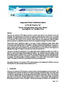
Figure 2: The VEVID Interface Mauga (2006) developed a Florida length-based vehicle classification scheme using the Support Vector Machines (SVM) supervised learning models. His team collected vehicle videos from Florida highways and used test vehicle length datasets to train the algorithm and classify vehicles. In that study, a rising trend in vehicle lengths has been identified - that is, vehicles from higher FHWA classes are likely to have longer lengths than vehicles belonging to the lower FHWA classes. Another fact is that there are considerable overlaps among classes in the length-based classification. The overlaps are particularly a discernible amount from class 2 up to class 7, and also from class 8 through class 11. Figure 3 further illustrates the identified problem where at least two areas of classification overlaps can be identified. It shows clearly that the length-based vehicle classification is incapable of distinguishing the FHWA scheme F vehicle classification (Mauga et al., 2006). Yu et al. (2009) compared the classification performance among Econolite Autoscope RackVision Terra sensor, Custom Electronic and Optical Solutions, The Infra-Red Traffic Logger (TIRTL) sensor, and Wavetronix SmartSensor HD. Both axle-based and length-based


8

classification schemes are used in their tests. A 15-class axle-based classification algorithm (Modified FHWA-15) was adopted for TIRTL sensor tests. This classification scheme combines all the classes in the standard FHWA-13 scheme plus additional Class 14 for unclassified vehicles or user-defined vehicle and Class 15 for road train with eight to 15 axles. The Hawaii Department of Transportation C5 length classification scheme was used to configure the classification bins of Autoscope sensor and SmartSensor HD (Yu et al., 2009). Their results showed that both SmartSensor HD and Autoscope provided inadequate vehicle classification accuracy for freeways. Congestion on the freeway may increase the failure rate of detected vehicles. In addition, lane changes under uncongested condition tend to cause double counts or misclassifications. TIRTL provides adequate accuracy for the FHWA axle-based classification and is particularly applicable for the detection of trucks and large vehicles at highways of industrial areas.

Overlaps in classes 8-11

Overlaps in classes 2-7

Figure 3: Florida Length Base Vehicle Classification Scheme Results using SVM Old Dominion University is currently working on a U.S. DOT sponsored project named “Exploring Image-Based Classification to Detect Vehicle Make and Model”. The project is aimed to perform vehicle classification at two levels: general classification of vehicles by size (car, truck, motorcycle, etc.) and specific classification of vehicles by make and model in the second level if the camera resolution allows (UI, 2012). Preliminary results from this study show that lengthbased classification of sedan, passenger truck/SUV, motorcycle, bus, small commercial truck, and large commercial truck has low successful classification rate. Their multi-class support vector machine (SVM) classifier shows an average accuracy of 74% with very poor classification rate between SUVs and small commercial trucks. However, the result with respect to the vehicle classification by make and model has not been reported and subject to video resolution. Little research has been reported in generating axle-based vehicle classification data by using the recently developed computer vision and image processing techniques. Frenzel (2002) proposed a video-based system in a heuristic study focused on truck detection and axle counting


9

rather than vehicle classification. The result shows that only 56% axle detection rate was gained by that system. No vehicle classification results were reported in that study. A couple of other studies (Messelodi et al., 2004; Buch et al., 2009) applied 3D model-based computer vision system for vehicle classification. The vehicles are modeled at a 3-dimentional level and then classified into classes. This method usually requires the developers to have extensive expertise in computer vision techniques, computer programming, and computing powers. However, such classification still produced misclassifications since one 3D model may have multiple axle configurations according to the FHWA scheme F. Zhang et al. (2007) used virtual dual-loop detectors within videos to mimic the functionality of loop detectors. It is significant for traffic data extraction at sites where dual-loop detectors are not available. However, this method, by its nature, still falls to the model-based approach. Therefore, it adapts the modeling errors pertained in the system. Kanhere (2008) attempted to develop video-based vehicle classification system using pattern recognition. The method is considered to use wheels as a feature object, but it did not provide a reference to classification using the axles and its configuration. Hsieh et al. (2006) used size and linearity features to dynamically classify vehicles from a built library. The classification is very library templates dependent and usually requires a considerable amount of time and efforts for the calibration process. Besides, the classification only has four bins which representing car, minivan, truck and van truck, respectively. Grimson (2005) attempted to classify vehicles from edge points of a detected vehicle object of video. They used pixel classification techniques to extract the vehicle shape. This effort is also library based and requires a long time for learning and recognizing vehicles. Recently, Yao et al. (2012) developed a computer vision-based software tool, namely, Rapid traffic Emission and energy Consumption Analysis (REMCAN) system. It enables a rapid vehicle operating mode distribution profiling for MOtor Vehicle Emission Simulator (MOVES) from video data. As a matter of fact, REMCAN lacks capability to extract the ground-truth vehicle classification as part of the MOVES emission source. The successful development of the RVIS will help to provide more reliable vehicle classification data to MOVES and therefore, enhance the accuracy of emission estimation. Even though in many studies, video-based technologies have been used to develop algorithms and tools to enhance the current vehicle classification performance, the methodologies are still limited due to their intrusive technology and algorithm dependent features. A hybrid method by combining multiple tools and technologies may produce better results from dealing with varied conditions than using single one tool or technology. Our preliminary sample study suggested that the hybrid vehicle classification (axle-based for light traffic and length-based for congestion) using computer vision and image processing techniques holds technical promise for vehicle classification under all traffic conditions.


10

CHAPTER 4: METHODOLOGY 4.1 Basic Concepts about Vehicle Classification 4.1.1 FHWA Scheme F Vehicle Classification (Axle-Based) FHWA classifies vehicles into the following 13 classifications, as illustrated by Figure 4 (ODOT 2011). 1. Motorcycles (Optional) - All two or three-wheeled motorized vehicles. Typical vehicles in this category have saddle type seats and are steered by handlebars rather than steering wheels. This category includes motorcycles, motor scooters, mopeds, motor powered bicycles, and threewheel motorcycles. This vehicle type may be reported at the option of the State. 2. Passenger Cars - All sedans, coupes, and station wagons manufactured primarily for the purpose of carrying passengers and including those passenger cars pulling recreational or other light trailers. 3. Other Two-Axle, Four-Tire Single Unit Vehicles - All two-axle, four-tire, vehicles, other than passenger cars. Included in this classification are pickups, panels, vans, and other vehicles such as campers, motor homes, ambulances, hearses, carryalls, and minibusses. Other two-axle, four-tire single-unit vehicles pulling recreational or other light trailers are included in this classification. Because automatic vehicle classifiers have difficulty distinguishing class 3 from class 2, these two classes may be combined into class 2. 4. Buses -All vehicles manufactured as traditional passenger-carrying buses with two axles and six tires or three or more axles. This category includes only traditional buses (including school buses) functioning as passenger-carrying vehicles. Modified buses should be considered to be a truck and should be appropriately classified. Note: In reporting information on trucks the following criteria should be used: • Truck tractor units traveling without a trailer will be considered single-unit trucks. • A truck tractor unit pulling another such units in a “saddle mount” configuration will be considered one single-unit truck and will be defined only by the axles on the pulling unit. • Vehicles are defined by the number of axles in contact with the road. Therefore, “floating” axles are counted only when in the down position. • The term “trailer” includes both semi- and full trailers. 5. Two-Axle, Six-Tire, Single-Unit Trucks - All vehicles on a single frame including trucks, camping and recreational vehicles, motor homes, etc., with two axles and dual rear wheels. 6. Three-Axle Single-Unit Trucks - All vehicles on a single frame including trucks, camping and recreational vehicles, motor homes, etc., with three axles. 7. Four or More Axle Single-Unit Trucks - All trucks on a single frame with four or more axles. 8. Four or Fewer Axle Single-Trailer Trucks - All vehicles with four or fewer axles consisting of two units, one of which is a tractor or straight truck power unit


Figure 4: FHWA Scheme F Vehicle Classification (ODOT, 2011)

11

12


9. Five-Axle Single-Trailer Trucks - All five-axle vehicles consisting of two units, one of which is a tractor or straight truck power unit. 10. Six or More Axle Single-Trailer Trucks - All vehicles with six or more axles consisting of two units, one of which is a tractor or straight truck power unit. 11. Five or fewer Axle Multi-Trailer Trucks - All vehicles with five or fewer axles consisting of three or more units, one of which is a tractor or straight truck power unit. 12. Six-Axle Multi-Trailer Trucks - All six-axle vehicles consisting of three or more units, one of which is a tractor or straight truck power unit 13. Seven or More Axle Multi-Trailer Trucks - All vehicles with seven or more axles consisting of three or more units, one of which is a tractor or straight truck power unit. 4.1.2 Length-Based and Bin-Based Vehicle Classification The length-based vehicle classification is usually redefined by bin class in applications. In other words, 13 types of vehicles, as defined by FHWA’s vehicle classification scheme, are regrouped into a number of bins based on length. In each bin, the lengths of vehicles are relatively close. For present applications, 3-bin or 4-bin scheme is defined. Table 2 provides detailed definitions of the 4-bin vehicle classification scheme. Figure 5 shows the graphical schematic of this 4-bin classification.

Table 2: 4-Bin Classification and Related Vehicle Types to Each Bin 4-Bin Classification

Bin Class

Vehicle Type (Group Class)

Length Range (ft)

Type 1: Motorcycles Personal Vehicle and Smaller Vehicles

Bin 1

Type 2: Passenger Cars (With 1- or 2Axle Trailers)

< 26

Type 3: Axles, 4-Tire Single Units, Pickup or Van (With 1- or 2-Axle Trailers) Type 4: Buses

Medium Trucks

Bin 2

Type 5: 2D – 2 Axles, 6-Tire Single Units (includes Handicapped-Equipped Bus and Mini School Bus)

26 - 39

Type 6: 3 Axles, Single Unit Heavy Trucks

Bin 3

Type 7: 4 or More Axles, Single Unit

39 - 65

Type 8: 3 to 4 Axles, Single Trailer Type 9: 5 Axles, Single Trailer Type 10: 6 or More Axles, Single Trailer Heavy and Large Trucks

Bin 4

Type 11: 5 or Less Axles, Multi-Trailers Type 12: 6 Axles, Multi-Trailers Type 13: 7 or more Axles, Multi-Trailers

< 65


13

Figure 5: FHWA classification scheme (FHWA, 2011)

For the 4-bin classification, a length based classifier to detect vehicle’s bin has proposed, and then the possible vehicle type will be determined based on the definitions of the identified bin. For example, if the length based classifier classifies a vehicle as the Bin-1, then the algorithm would determine the vehicle type to be either type 1, or 2, or 3. For the group classification, we proposed a hybrid technique using the length of the vehicle and the number of tires. The number of tires counts how many tires a vehicle has on one side which can be interpreted as the number of the axles of the vehicle. Therefore, we propose a length based method for 4-Bin classification and a hybrid length based and number of axle method for group classification.


14

4.2 Image Processing Methods for Extracting Vehicle Length and Axles 4.2.1 Challenges for Finding Vehicle Length and Positions of Vehicle Tires Figure 6 shows the main blocks of the developed system to extract the essential features of a vehicle and classify it into 4-bin length-based classification from video data. The video data was obtained through filming the traffic at I-275 in Cincinnati area, Ohio and details about the video data collection will be presented in Chapter 5. In this section, a brief overview of the proposed methodology and technical details will be presented.

Figure 6: Proposed Method Overall Scheme

The first step of our system is detecting motions in frame sequences. A video consists of sequential frames. There is a variety of techniques which can be used to find motions in the frame sequences. However, a variety of challenges may be faced off as a motion detection technique is being developed, such as:        

Moving Background: For example, when the leaves of a tree are moving by the wind. Cast Shadow: For example, shadow of the vehicles on the road. Camera Jitter: In an outdoor environment most of the time wind causes the stationary camera to move a little bit. Gradual light changes: For example, going from daylight to night. Sudden light changes: For example, clouds suddenly covering the sun. Camouflage: It happens when the foreground object is similar to the background like a gray vehicle on a road. Bootstrapping: Some algorithms need to have a complete set of the background scene, those algorithms cannot be adopted through the time. Though algorithms cannot overcome all these issue.

Although the computing algorithms cannot overcome these issues completely for some technical reasons, an efficient moving object detection is usually aimed to minimize these issues. In general, there are three major categories of the motion detection algorithms as follows: 

Optical Flow: When the algorithm finds an object as a motion object based on the features of the objects, such as edges, characteristics of its surface, it tries to follow the motion object. This technique has some advantages to being good for scenarios as the camera is


15

moving. But it is not well-suited for stationary cameras because of its cost concern. The Optical Flow technique also has other disadvantages; for example, it requires a significant amount of computation that makes it very time consuming and needs special hardware to be implemented in real time; it is very sensitive to illumination changes, and so forth. 

Temporal Differencing: This technique detects moving objects by calculating the differences between pixels in consecutive frames. Unlike the optical flow, this algorithm can be implemented in real time and it is not costly in regards to process time. However, it has its own disadvantages which we can name a few. For example, relevant pixels cannot be extracted so well; if the moving objects moves slowly it may become part of the background and will not be recognized correctly.



Background Subtraction: This technique uses consecutive frames to build a background model. After coming a new frame, it gets compared against the background model and the pixels with a lot of differences in intensity are foreground pixels. The disadvantage of the Background Subtraction technique is that it takes time to create the background model. Background Subtraction technique is the one that we have used in this study because it has a lot of advantages compared to other techniques. Unlike optical flow, it is fast and accurate, and unlike Temporal differencing, it is able to detect relevant foreground objects. There are several approaches to implement a background subtraction method, like codebook (Kim, 2005), Kalman filter (Boult et al., 1999), Single Gaussian model (Gordon, 1999), and Gaussian Mixture Models (GMM) Stauffer et al., 2000). Among these approaches, GMM is the most popular algorithm in the literature. GMM can overcome the issues which were mentioned before properly. The details about this technique will be discussed in the next section.

The second step of the developed system is Tire Region Extraction. After Finding the moving object (in our case vehicle), it is feasible to find the length of the object and extract tires region. Tires region can be approximated by finding the bottom corners of the vehicle. By finding the bottom corners and having the vehicle length, a box which includes tires can be approximated. The third step of our system is finding tires in its tire region. Having the tire region box (a cropped image of the frame includes only tires part of the vehicle), we need to implement an image processing technique to find the tires in it. The one that is used in our system is based on the tire contour features. Contour is a sequence of points which is around an object. We find all the contours in tire region and reject those which are unlikely to be a tire and the remained ones (valid ones) are recognized as vehicle tires. Valid contours can be counted and also the center of the contour is the position of the tire. The fourth and the last step of our system is the classification step. In this step, the length of the vehicle and the positions of the tires are extracted. The length of the vehicle helps to classify into the 4-Bin classification and the length plus the position of the tires help to classify in group classification. The following four steps, namely, object detection, tire region extraction, tire extraction, and classification, are the main flow of our developed system. In each step, other algorithms are


16

used to make that step more precise. In the next section, details about each major techniques are discussed.

4.2.2 Step 1 - Object Detection Figure 7 shows the scheme over the first step. In this step, a Gaussian mixture model has been used to model the background. When a new frame arrives, it gets compared to this model and its pixels get classified as background pixels and foreground pixels. On the classified pixels, a morphological operator has been applied to connect the relevant pixels together and get rid of the noisy pixels which classified incorrectly or they are so small. After that, a binary (black and white) image is obtained. The white part indicates of the foreground object and the black part indicate background. It should be noted that until now just a black and white image is obtained and still the objects as an array of points is not defined. Therefore, we take the contours of the binary image out. This gives a set of arrays. Each element of this array is a foreground object and each object includes the location of pixels around the object. Therefore, the objects in the image are now obtained and they are stored in an array. The technical part of GMM, Morphological Operator, and Contours will be discussed in the following sections.

Figure 7: Foreground Object Detection Scheme 4.2.2.1 Introduction to Gaussian Mixture Models Background Subtraction In Background subtraction using Gaussian Mixture Models, rather than modeling each pixel with one model (mean and variance), the mixture of Gaussian models are employed. The usual model

17


number is 3. Therefore, each pixel has 3 Gaussian models. Pixel values that do not fit the background Gaussian distribution are considered as foreground. This system can adapt to deal with lightning changes, repetitive motion of background objects, slow-moving objects (Bradski et al., 2008). 4.2.2.2 Background Maintenance by Gaussian Mixture Models A quick Gaussian Mixture Models algorithm is presented in the study and described below: 1. Initialize: Choose the number of Gaussians and a learning constant : values in the range 0.0.1-0.1 are commonly used. At each pixel, initialize Gaussians ,∑ , is normal distribution, with mean vector and covariance matrix ∑ , and corresponding . Since the algorithm will evolve this may be safely done crudely on the weights understanding that early measurements may be unreliable. 2. Acquire frame , with intensity vector – probably this will be an vector , , . Determine which Gaussian match this observation to be within, say, 2.5 of the mean. In the multi-dimensional case, a simplifying assumption made for computational complexity reasons: the different components of the observation are taken to be independent and the equal variance allowing a quick test for ‘acceptability’. 3. If a match found as Gaussian : a) Set the weights according to:

1 ,

(2)

And re-normalize. b) Set | ,

(3)

And ,

1 1

4. If no Gaussian marched ,

,

(4) ,

: then determine

(5)

,

argmin

and delete

. Then set (6)

18


2 ,

(7)

0.5

(8)

The algorithm is reasonably robust to those choices. 5. Determine as in: argmin ∑

,

(9)

If the best matched Gaussian model is a background model, the pixel will be considered as a background pixel. If the best matched Gaussian model is a foreground model, the pixel will be considered as a foreground pixel. 6. Use some combination of blurring and morphological dilations and erosions to remove very small regions in the difference image, and to fill in ‘holes’ etc. in larger ones. Surviving regions represent the moving objects in the scene. 7. Return to (2) for next frame (Sonka et al., 2008). Figure 8 demonstrates an example result of this technique.

Figure 8: Example Result of Gaussian Mixture Model Approach 4.2.2.3 Morphological Operators As it is mentioned before, the result of the GMM algorithm contains noisy components. The noise can be eliminated by morphological operators, typically, erosion and dilation. With applying these

19


two operators, this technique will fill the holes when a foreground object has some holes in it. If some small foregrounds detected which were not connected to a big foreground object it will be eliminated. Erosion on a binary image can be expressed as: ⊖

⋂

∈

(10)

Where, A is a binary image. We should note that in a binary image 1 represent as white and 0 represents, and B is a 3 3 matrix with a center anchor and value of one for each element and gets convolved with the entire image. Figure 9 shows an example result of this operation on a binary image. It can be seen that this operator was able to eliminate the noisy part (small white part).

Figure 9: Result of Erosion Operator on A Binary Image

Dilation can be expressed as: ⊕

⋃

∈

(11)

Where A is a binary image. We should note that in a binary image 1 represent as white and 0 represents and B is a 3 3 matrix with a center anchor and value of one for each element and gets convolved with the entire image. Figure 10 shows the result of this operation on a binary image. It can be seen that this operator was able to connect the relevant parts (the text part). This technique is employed for getting clear foreground object. Therefore, all the unnecessary foreground (small changes) can be eliminated and relevant pixels get connected. Figure 11 shows the result of applying erosion and dilation on the system. It can be seen relevant points have got connected and noisy pixels have got cleaned properly.


20

Figure 10: Example Result of Dilation on A Binary Image

Figure 11: Example Result of Morphological Operator Note: Top Image is the original image and the bottom image is the process of GMM background subtraction and morphological operators


21

4.2.2.4 Contours There is a variety of approaches in image processing to detect the edges of the object. One of them is called Canny Edge Detector. In a glimpse canny edge detector consists of five steps: 1. 2. 3. 4. 5.

Apply Gaussian filter to smooth the image in order to remove the noise Find the intensity gradients of the image Apply non-maximum suppression to get rid of spurious response to edge detection Apply double threshold to determine potential edges Track edge by hysteresis: Finalize the detection of edges by suppressing all the other edges that are weak and not connected to strong edges.

Every step has its mathematical approach and more details about could be found in Bradski’s book “Learning OpenCV: Computer vision with the OpenCV library” (Bradski, G., and Kaehler, A., 2008). Figure 12 shows the result of canny edge detector on a binary image.

Figure 12: Result of Canny Edge Detector on A Binary Image A contour is an array of points which represents a curve in an image. The result of canny edge detector is an input for finding the contours of that image. A white point (an edge point) will be found and tracked and all the points connected to that point will be a contour. Therefore, after


22

finding contours on the binary image we can have a set of objects which every object have all the points in its curve. The final result is to have the contours array and the segmented vehicle. Figure 13 shows samples of segmented vehicles obtained through this method.

Figure 13: Samples of Segmented Vehicles

4.2.3 Step 2 - Tire Region Extraction Figure 14 shows the flowchart for processing vehicle cropped images. The bottom corners of these images need to be identified in the process through converting these images to grayscale images in order to get the edges and then the contours out of them. With a precise look, it can be seen that these pictures have a lot of unnecessary edges which make them too complex to process. The way to tackle complex scene problem in the study is Mean Shift Color Segmentation. Mean shift color segmentation is a segmentation technique that assigns only one color to the entire region which has similar intensity. For example, intensity 123 is similar to 125 but they are not the same. If


23

these two intensities are in the same region both of them will be assigned to the same intensities like 124. The detail about this algorithm will be discussed in the 4.2.3 section. As shown by Figure 14, the results of step one are the segmented vehicle images and the contour around them. A mean-shift color segmentation is applied to vehicle’s image to make the similar regions homogenous. A sharpening method is applied on homogenous image to make the edges sharper (Sonka et al., 2008). After that, the resulted image with sharped edges is converted to grayscale and edges get extracted to find the image’s contours. As it mentioned before, a contour is a list of points representing a curve but we are interested in finding the corners of this curve. There is an algorithm called Ramer-Douglas-Peucker (RDP) that can be helpful to finding the corners on a curve. The idea of this algorithm is to find another curve similar to the original curve but with fewer points. The details about the RDP will be discussed in 4.2.3.2 section. Based on the corners obtained from RDP algorithm we find the appropriate two bottom corners. Finding these two bottom corners will be discussed in 4.2.3.3 section. When the bottom corners get picked, it is feasible to create a bounding box for the tire region. Figure 14 shows a sample of finding contour with related corners.

Figure 14: Step 2 Scheme

4.2.3 Mean-Shift Segmentation Any pixel has a feature space consists of quantitative intensity levels which based on the color space can be mapped into a multi-dimensional space with other pixels. Once all the pixels’ of an image is mapped to the multi-dimensional feature space, the feature space is more densely populated in locations corresponding to the image features. These locations form cluster clusters which in the image each cluster may correspond to image objects based on what multi-dimensional feature space representations (FHWA, 2011). In our case, the feature space will be the color feature , , , , or , , , , which , is pixel location in the image. space, Figure 15 shows the principle of mean shift algorithm on just one cluster (Sonka et al., 2008).


24

Figure 15: Illustration of Principle of Mean Shift Algorithm Notes: (a) Initial region of interest has chosen randomly. (b)Algorithm will find a new mean shift for the data under the circular window. (c) By repetition of part (b) it, mean shift gets closer to the denser region which is density local maxima (Sonka et al., 2008). 4.2.3.1 Principle of the Mean Shift Procedure The densest region of data is identified in an iterative process: (a) The initial region of interest is randomly positioned over data and its centroid is determined. The new region is moved to the location of the identified centroid. The vector determining the region's positional change is the mean shift. (b) Next step of the mean shift procedure: a new mean shift vector is determined and the region is moved accordingly. (c) The mean shift vectors are determined in the remaining steps of the procedure until convergence. The final location identifies the local density maximum, or the local mode, of the probability density function (Sonka et al., 2008). Figure 16 shows some results of this technique on other application we can see that this algorithm was able to distinguish parts of an image based on their color. What is expected from this algorithm is that segment only the foreground objects that we have. Therefore, tires, hubs, exterior part of the vehicle, truck and trailer can be separated so after that we will be able to analyze each part which will leads to a better classification even in axle-based classification. Figure 17 shows the result of mean-shift segmentation on our system.


Figure 16: Example of Applying the Mean-shift Segmentation Notes: Left side: Original Images; right side: segmented images based on mean-shift segmentation (Coifman 2012)

Figure 17: Sample Result of Mean-shift Segmentation using Studied Data

25

26


4.2.3.2 Ramer-Douglas-Peueker (RDP) The idea behind this algorithm is to find a curve similar to the original curve but with fewer points. In this algorithm, the user defines a as precision. The curve has a starting point and an ending point. A straight line between two points will be assumed. The furthest point between these points from this line will be picked. If the distance from the line is less than , this point will be ignored. If the distance is greater than , this point will be a new end point from the original start point to this new point, and a new start point from this new point to the original end point as well. This algorithm iteratively goes around until no new point can be found. Figure 18 illustrates how the RDP works in one iteration (Wikipedia, 2015a).

Figure 18: The RDP Algorithm Scheme

4.2.3.3 Finding Two Bottom Corners and Tire Region For the bottom-left part as shown in Figure 19, the left most corner has been chosen (i.e., the least distance from the y-axis). For the bottom-right part, the corner that has the least distance from the bottom-right part of the image is chosen. These two distances have been shown with yellow color in Figure 19. In relating to the bottom- left corner and the bottom-right corner of the vehicle, and the size of the cropped image (vehicle object), a box representing the region of interest can be found. If the size of the vehicle is big, thus, the size of the region of interest will be big and if the size of the vehicle is small the size of the region of interest will be smaller. 0.03

(12)

0.03

(13)

27


(14)

Figure 19: Result of Finding Corners on Contours Based on RDP Note: The green dots are the corners

(15) 2

(16) (17) (18) (19) 7 7

(20) (21) (22) (23)

(16), (17), (18), (19), (20), (21), (22), (23) are the coordinates of the region of interest box. and are relative to the vehicle size, thus if the vehicle size is large the region of interest will be large, and vice versa. (14) is the slope of left and right bottom corners and (15) is the intercept. These relations have been used in our system to find the appropriate box around the tire region. The two top corners are blue dots and the two bottom corners are red dots in Figure 19. The result of finding this bounding box in our system is shown in Figure 20.

28


Figure 20: Sample Result of Finding Tire Region with Study Data

4.2.3.4 Standard Vehicle Length The length between two bottom corners can represent the length of the vehicle. There is a problem here this length is affected by perspective and the length of the vehicle between different frames varies. And as the vehicle gets closer to the camera this length becomes larger. To overcome this problem we made a practical technique. There are two points for two corners, begin of the vehicle 1, 1 , and end of the vehicle (x2,y2). The trick is for calculating r1 and r2, we gave weight to distance x and y because of their depth effect. Now instead of using a simple Euclid distance, the weighted Euclid distance will be calculated. 1

1

1

(24) 2

2

2 (25)

(26) (27)

29


(28)

In this formulation, and are the coefficients with an attempt to put the gravity of depth into Euclid distance. gives the ratio of beginning and ending points of the vehicle to the standard point (a point which every distance gets compared to). The is the length that perspective effect has got discarded. Figure 21 shows the realization of the points that we discussed in the formulation. In our system is equal to 1 and is equal to 8.

Figure 21: Standard Length Calculation

4.2.4 Step 3 - Tire Extraction As discussed earlier, Figure 20 shows the overall flow over the tire extraction step, and Figure 21 is cropped part of the original image. In the study, the color segmented image is used to distinguish the objects. In the previous step, the tire region gets extracted, and in this step the tire region gets converted to grayscale image in order to find the contours. The detailed calculation items are shown in Figure 22. Figure 23 shows a sample result of finding contours.


30

Figure 22: Step 3 Scheme

Figure 23: Sample Result of Finding Contour in Tire Region

4.2.4.1 Tire Contour Conditions A number of rules have been applied for the found contours in order to find perfect tire candidates. The rules are: 1. The box should not be too narrow if 0.2

1.5

2. Large size contours cannot be tire candidates if 100 3. Small size contours cannot be tire candidates if 20 4. The distance between centers of two accepted contours should be more than 20 pixels The result of these contour selections can be seen in Figure 24. Now that we selected the candidates if the number of candidates is less than two we add another one to wherever side which does not have contour and if it is more than 3 contours it might be a possibility that we have noisy selected contour. Since all the centers should be on a straight line we put a fitting line over all the centers and the one with more than , which is the threshold, that one can be considered as noisy and gets rejected.

31


2 3 3

(29)

(30) It can be seen in Figure 24 that a contour was detected as noise and got rejected because it was far from the fit line.

Figure 24: Result of Contour Selection. Note: The green boxes are finally approved and the only red one is noisy and rejected

4.2.4.2 Fit Line Fitting a line through some points can be achieved by minimizing Equation (30). ∑ Where is the distance between the couple of more examples for this step.

(31) point and the line (Wikipedia, 2015). Figure 25 shows a


32

Figure 25: Sample Result of Step 3

4.2 5 Step 4 – Vehicle Classification In the study, we are testing two vehicle classification methods: 4-bin length-based classification and axle-based classification. In the study, the video data allows us to focus on one side of the road only. We also have processed a portion of that road since the perspective effect in a distance far from the camera will not give us full information about vehicle appearance. Therefore, we decided to process the region that is near to the camera and the vehicle can be seen properly. Figure 26 shows the process region. Inside of the red polygon, we take the standard vehicle length and also process the number and position of the tires. It is obvious that each vehicle can appear in more than one frame. Therefore, it is necessary to find out which vehicle is the same vehicle in the previous frames. For this purpose, we need a technique to find the same vehicle in the frame sequences and this technique is called Object Tracking.

33


Figure 26: Process Region (inside the red polygon)

4.2.5.1 Object Tracking Since we are processing one side of the road, we know that the location of the vehicle in the next frame should be greater than location of the vehicle in previous frame. This is the first condition of our tracking.

(32)

Another condition is that they have to be similar. Therefore, we need a technique two find similarity between to objects. Figure 27 shows the same vehicle in two consecutive frames.

Figure 27: The Same Vehicle in Two Consecutive Frames


34

To find the similarity between two objects, a technique named Histogram Matching is used. Histogram matching gives a floating number between 0 and 10. If the objects are similar in their color distribution the number is closer to 0 and if they are not close to each other the number is close to 10. The details about this algorithm will be discussed in 4.2.5.2 section. In our system, this number should be less than 0.3 to be considered similar. In summary, for each vehicle an array is allocated and after each frame the new objects get compared against these arrays and the array with the most similarity and the similarity number under 0.3 can be considered as the same vehicle. We should note again that the location of the vehicle next frames should be further than the previous frames. 4.2.5.2 Histogram Matching Every frame in our system is represented in color space. color space consists of three planes red plane, green plane, and blue plane. But the closest color space to human color understanding is color space. Figure 28 shows HSV color space (Wikipedia, 2015b). We should note that Hue varies from 0 to 179 and Saturation varies between 0 and 255. In our system we divided hue into 50 bins it means an element with hue equals to 4 and another element with hue equals to 9 falls into the same bin. Also, we divided saturation into 60 bins. And also in this algorithm we do not use Value because we do not want the brightness of a color impact our judgment. Therefore, a certain color between two frames can be brighter or darker. After obtaining the Hue and Saturation plots of two objects in different frames, we compare the error between these two plots and the error between theses plots is our similarity. Therefore, similarity close to 0 means the two pictures are more similar to each other and further from 0 means they are not so much similar to each other (Bradski, 2008).

Figure 28: HSV Color Space (Wikipedia, 2015b)

35


4.2.5.3 4-Bin Length-Based Classification and Axle-Based Group Classification The length distribution for vehicles is: 1 2 3 4

160 260

160

360

260 360

(33)

After it was defined a vehicle belongs to which of the bins, it is time to find the group for the vehicle based on Table 2. If the vehicle is in Bin-1: 1 3 2

2

70 104

(34)

The group classification in Bin-1 is only based on length. If the vehicle is in Bin-2: 4 5

2

3

(35)

If the vehicle is in Bin-3: 8

3 4

7 6

4 3

1 2 2 2 1 3 (36) 3 1

If the vehicle is in Bin-4: 10 11 12 13 9

6 5 6 , 7 5 ,

, , ,

3 3 3 6

(37)

These rules are applied in the study for 4-bin length-based classification, which is then further split into sub-groups, as shown by Equations (34) through (37).


36

CHPATER 5: DATA COLLECTION 5.1 Data Collection Site and Time The video data was collected at a place near I-275 close to traffic monitoring station 626 in Cincinnati area, Ohio. The GPS floating car data was collected on the routes on the I-275 between Exit 44 and Exist 47. The traffic monitoring station 626 is located near Exit 47. The video data and GPS data collections were conducted between the dates 5/19/2014 to 5/26/2014 (he data was not collected for half a day on 5/20/14 due to showers). The data was collected from 19th May 2014 (Wednesday) through 26th May 2014 (Sunday). The traffic was filmed via a video camera from 8:00 AM to 6:00 PM. Meanwhile, the GPS-based floating car data was collected during peak hours. There were frequent showers in the morning period which caused delays in starting the video in the morning time. 5.2 Video Data Collection The video cameras were placed on the turf between the ramp and freeway to record freeway traffic. The cameras were mounted 14 feet above the ground over the scissor lift. The orientation of the cameras was placed in such a way that the substantial extent of the freeway is captured as per requirements. Two cameras were used to capture the traffic in different angles. Figure 29 shows the location of the video camera and the capture recording field of the camera. A complete log of all the capture data was also maintained. Table 3 shows the duration of the videos captured. A total of 87 hours of video was recorded in these days.

Figure 29: Video Camera Placed near I-275 Close to Traffic Monitoring Station 626


37

The scissor lift was used to mount the cameras. The cameras were mounted about 12-14 feet above the ground and the videos were captured. Two cameras were placed on the scissor lift for the two different orientations. Figure 30 shows the two cameras mounted on the scissor lift. Figure 31 shows the exact location of the deployed equipment. Two cameras were placed adjacent to each other facing different directions. Table 3: Total Number of Hours of Video Data Captured Date 5/19/2014 5/20/2014 5/21/2014 5/22/2014 5/23/2014 5/24/2014 5/25/2014 5/26/2014 Sum

Camera 1 3hrs 45 min 3hrs 34 min 7hrs 48 min 7hrs 22 min 3hrs 44 min 7hrs 30 min 8hrs 10 min 7hrs 30 min

Camera 2

3hrs 20 min 7hrs 40 min 4hrs 7hrs 10 min 7hrs 55 min 8hrs 10 min

Total hours 3hrs 45 min 3hrs 34 min 11hrs 8min 15hrs 2min 7hrs 44 min 14hrs 40min 16hrs 10 min 15hrs 40min 87hrs 10 min

Figure 30: Two Cameras Mounted on the Scissor Lift


38

Figure 31: Exact Location of the Deployed Equipment 5.3 GPS Data Collection The GPS data logger was switched on at Exit -44 of I-275 East. From Exit- 44 the car was driven till the Exit- 47 of I-275 East is reached. At the exit, left of the fork at the exit is taken and following the signs for Reed Hartman Highway and finally merging into I-275 West to complete the trip. The car was driven in cruise mode mostly so as to maintain a constant speed all over the trips. Floating car runs were carried at least 3 times. Effectively, the data collection route is the floating runs between the exit-44 to exit-47. The runs were carried depending on the weather conditions. Timings were noted at the respective locations, i.e. when the vehicle is at the camera and at exit44 while carrying the runs. The complete route is shown in Figure 32. Table 4 shows the sample GPS trip log of the 5/20/2014. In addition to this, markers were attached to the vehicle on the wind shield so that it can be used for the VEVID software for validation.

Figure 32: Overview of the Complete GPS Data Collection Route

39


Table 4: Sample Log of the Floating Car Runs Recorded on 5/20/14 Trip Number Trip 1 Trip 2 Trip 3 Trip 4

Start time at Exit-44 3:02PM 3:13PM 3:24PM 3:35PM

Time at Camera 3:04PM 3:15PM 3:26PM 3:37PM

Speed (mph) 60 60 60 60

The total number of Floating car runs (GPS trips) that were carried are shown in Table 5. More numbers of trips were taken in the afternoon as the shadow of the vehicles were not prominent, which in turn would be helpful to develop the algorithm.

Table 5: Total Number of GPS Round Trips Date

Morning

Afternoon

5/19/2014

1

4

5

5/20/2014

1

5

6

5/21/2014

3

4

5/22/2014

3

4

7

5/23/2014

3

4

7

5/24/2014

3

5

2

10

5/25/2014

3

5

2

10

5/26/2014

3

6

3

10

Sum of Trips

Evening

2

Total

9

64


40

CHAPTER 6: TESTING EVALUATION In this chapter, the applicability of the proposed approaches that have been presented in Chapter 4 will be discussed through a sample study of applying the approaches with sample data as discussed in Chapter 5. In the testing study, a single video is selected to take out vehicle samples from it and evaluate the performance of the developed algorithm. With the selected video, the perspective effect has been calculated and the process region has been selected. Different types of measurements will be introduced in this chapter to evaluate the performance of the algorithm from different perspectives. Those measurements will be introduced and defined in details in the chapter. And the performance evaluation will show how the method works in vehicle classification from videos with respect to 4-bin length-based classes and axle-based group vehicle classes. 6.1 Measurement Criteria In order to well assess the performance of vehicle classification and identify the problem feature when a wrong identification occurs, the following four indicators are defined to constitute the performance measurements: 1. True Positive (TP): the TP indicator is measured by the number of samples which are correctly classified into their respective classes. In our example, if the samples which are Bin-1 and the algorithm classified them as Bin-1, the number of these samples is the value of the TP indicator. 2. True Negative (TN): the TN indicator is measured by the number of samples which are correctly rejected for a certain class. For example, if the number of samples which are not in Bin-1 and the algorithm did not classify them into Bin-1. The number of these samples is the value of the TN indicator. 3. False Positive (FP): the FP indicator is measured by the number of samples which do not belong to the class, but the algorithm incorrectly classified them into the class. For example, if the number of samples which does not belong to Bin-1 but the algorithm wrongly put them into the class of Bin-1, the number of these samples is the value of the FP indicator. 4. False Negative (FN): the FN indicator is measured by the number of samples which do belong to the class, but the algorithm incorrectly rejected them or did not put them into the class. For example, if the number of samples which belong to Bin-1 but the algorithm did not put them into the class of Bin-1, the number of these samples is the value of the FN indicator.

41


Each class has values of those four indicators. In order to further reveal in-depth relationship between the errors and samples on each vehicle class, the following indexes are defined and can be measured by the above four indicators 

Sensitivity: (38) The Sensitivity means the correct classification by the algorithm over all the samples from a certain class (the denominator is correctly classified samples added to the samples in the same class, but the algorithm could not recognize them). Sensitivity relates to the algorithm’s ability of correctly classifying a sample within that class. For example, of 7 Bin-1 vehicles the algorithm correctly identifies 5 of them as Bin-1. The sensitivity is then 0.71. It means the possibility of 71% by the algorithm to identify the calculated to be Bin-1 class.



Specificity: (39) The Precision means the correct classification by the algorithm over all the samples that the algorithm is able to identify as a certain class (the denominator is correctly classified samples added to incorrectly classified samples by the algorithm). Precision implies the ability of the algorithm to catch more relevant samples related to a specific class (or miss fewer identifications). For example, there are 7 Bin-1 vehicles in the concerned sample, but the algorithm identified 13 Bin-1 vehicles, including 5 correctly identified Bin-1 vehicles. It is obvious that 8 of them are not Bin-1 vehicles but wrongly identified as Bin1 vehicles (i.e., false positive). Therefore, the sensitivity remains 71% (i.e, 0.71) but 0.53. It means the ability of the algorithm to classify relevant samples the precision is over Bin-1 is 53%. If a classification algorithm has a tendency to classify the samples into one specific class, all samples or most of them get classified as that certain class. Thus, it is highly probable that class will get a high sensitivity. On the other hand, since the algorithm has a tendency to that class, a lot of samples that does not belong to the class carelessly classified as that class. In this case, although the sensitivity for that class is high, the precision will be low. Therefore, an algorithm may have a high Sensitivity with a low Precision for a certain class of vehicles. In other words, a good algorithm should have high sensitivity and high precision in the same time.



Harmonic Mean of Two Numbers, x1 and x2. (40)

42


Where and are two integers A is the Harmonic mean. Also, F1 measure is a harmonic mean of two integers and those two integers are precision and sensitivity. 

F1 Measure: 1

(41)

If 1 is high, it means the algorithm has a good precision and sensitivity in the same time. 6.2 Testing Results 1185 samples are selected in the test study. Table 6 shows the overall performance of the developed method. Table 6: Overall Performance of the Method Samples

True Positive

Average

4-Bin Length-based Classification

1185

1079

91%

Axle-based Group Classification

1185

856

72.2%

It can be seen that algorithm had a better performance in 4-Bin length-based classification than the axle-based group classification. There may be two reasons why this result is obtained. First, when a vehicle gets misclassified in 4-Bin classification, it definitely would be misclassified in axle-based group classification. The error of the 4-Bin classification will propagate to the axlebased group classification. Second, there may be some noises in the process for finding the tires and number of tires. The performance for each individual Bin class is also investigated. Table 7 summarizes the performance for each Bin classification. Table 7: Method Performance for Each Individual Bin Class Total

TP

FP

TN

FN

Sensitivity (%)

Precision (%)

F1 (%)

Bin-1

911

842

4

270

69

92.4

99.5

95.8

Bin-2

90

84

89

1006

6

93.3

48.5

63.8

Bin-3

54

25

3

1128

29

46.2

89.2

60.9

Bin-4

131

128

10

1044

3

97.7

92.7

95.1

It can be seen that the algorithm has high F1 for Bin-1 and Bin-2. It means the algorithm is successful in classifying between these two Bins. Also, it can be seen that Bin-2 has high Sensitivity. Most of the Bin-3 samples were correctly identified, but Bin-2 has a low Precision, which means a lot of other samples that did not belong to Bin-2 has been actually classified as Bin-2. On the other hand, Bin-3 has a low sensitivity, which means the algorithm failed to classify

43


a great amount of Bin-3 samples. And Bin-3 has a high precision, which means there are not a lot of other samples from different classes that have been identified as Bin-3 by the algorithm. Each axle-based group class was also investigated separately. Because some types of vehicles were not observed with sufficient size of samples, it’s not significant to come to solid conclusions for those classes of vehicles, as indicated by Table 8. The evaluation results are provided in Table 8. Table 8: Method Performance for Each Axle-Based Group Class Total Class Group-1 Class Group-2 Class Group-3 Class Group-4 Class Group-5 Class Group-6 Class Group-7 Class Group-8 Class Group-9 Class Group-10 Class Group-11 Class Group-12 Class Group-13

TP

FP

TN

FN

Sensitivity (%)

Precision (%)

F1 (%)

Lack of Samples 586

435

21

578

151

74.2

95.3

83.4

319

250

133

733

69

78.3

65.2

71.2

Lack of Samples 94

88

75

1021

6

93.2

52.5

68.4

52

24

3

1130

28

46.1

88.8

60.7

Lack of Samples Lack of Samples 113

58

17

1055

55

51.3

77.3

61.7

9

4

26

1150

5

44.4

13.3

20.5

Lack of Samples Lack of Samples Lack of Samples

It can be seen from Table 8 that the 4-Bin length-based classification is more successful than the axle-based group classification. As mentioned earlier, the first reason is the error propagation of 4-Bin classification to the group classification, and the second reason is the error from the Tire Extraction step. The most successful Group classification is Class Group-2 with an F1 measure of 83.4%. However, F1 measure for Class Group-10 is 20.5% and there are only 9 samples. Therefore, no conclusion can be made for Class Group-10, only based on such a small sized sample.


44

CHAPTER 7: DISCUSSION In the study, the use of machine vision and image processing techniques in vehicle classification has been investigated. Three major problems are identified remaining unresolved. First, when two or more vehicles are close to each other, they visually get overlapped in the video frame, as shown in Figure 33. As a result, the algorithm is unable to distinguish them. Figure 36 shows an example of two cars “merging” together with a big truck. The identified object is the truck only without identification of the other two cars.

Figure 33: Example of Visually Overlapped Vehicles

Second, a vehicle is tracked by comparing its similarity to the previous frames; however, this similarity may not be identified when a vehicle is partially overlapped with other vehicles in images, or as the similarity gets compromised even though it is referred to the same vehicle. The current technique may have difficulty to identify a vehicle to be similar to the same vehicle in the previous frame, because of changes in color distribution. A great amount of changes in vehicle color distribution may result in failure of finding the same similarity in the next frames. Figure 34 shows an example of color distribution changes.


45

Figure 34: Example of Color Distribution Changes The third problem is that our algorithm is highly dependent upon the appearance and vehicle colors. Thus, any conditions regarding having low contrast and low brightness will result in lower performance. Therefore, it is of high importance that camera should be placed somewhere with enough light projectors for dark hours of a day. More details about those challenges and their possible solutions will be discussed in 8.1 Section.


46

CHAPTER 8: FUTURE WORK 8.1 Challenges Some challenges are still existing and new investigations are needed on the basis of the results of this reported study. Most notably, key factors are related to adversary weather conditions, low light condition, vehicle occlusion, and camera viewpoint. Due to funding and time limit of the project, no opportunity has been available to explore those questions in the study. Despite it, the study suggests some ideas to be considered in the future work. 8.1.1. Adversary Weather Conditions and Low Light Condition Right now, our system has been tested for more than one thousand vehicles under good weather condition. Since the algorithms involved in our developed system highly depends on color changes (e.g., the background subtraction, the vehicle tracking), a major problem in bad weather conditions like foggy, rainy, snowy, and so forth. In addition, vision is not reliable at night for contrasting colors, and also, the vehicle's lights would change the color of the road, and as a result, part of the road may be identified as a foreground object which is actually not wanted. Therefore, using an infrared camera and improving the tracking algorithm based on color and location as to be based on location only could be a feasible solution to these problems. Since changing the visible band camera to an infrared camera may have side effects on axle-based classification, the axle based method should be disabled. As a result, there will be a payoff between having not enough light or bad weather conditions and the accuracy of the system. In other words, new experiments should be conducted to analyze the tolerance and accuracy of the system under different weather conditions with different lighting conditions. 8.1.2. Occlusion In this study, when a vehicle in the closest lane to the camera occludes a part or the full segment of another vehicle in a different lane, the occluded vehicle gets ignored and would not be identified by the algorithm. Therefore, only the front vehicle would be identified while another vehicle would be neglected. In addition, an experiment is needed to measure the accuracy of the algorithm against different traffic volumes. For all the vehicles at varied lanes, a top-view camera may be a feasible solution. A top-view camera does not necessary obliterate the axle-based classification. A top view camera with a certain angle to the road (e.g. 45 degrees with respect to the land) can preserve the axle-based classification and 4-Bin length classification. On the basis of the procedure proposed in the study, a new algorithm is required to separate the vehicles from each other. In scenarios that the tires are not visible to the camera, the algorithm can identify the vehicle type by vehicle length only. Therefore, a top-view with a certain camera angle experiment is suggested for the future work.


47

8.2 VIEW-TRAFIC The proposed method is the core engine of an RVIS model. The RVIS is an assistant aid to the proposed “hybrid” vehicle information extraction to processing vehicle classification and extracts other travel features in an automatic way. However, the testing has proved that the RVIS seems to perform well under light traffic only and would have higher error rate against congested traffic. Another model VEVID that was developed previously by the authors has an advantage over the RVIS in extracting trajectories of all categories of vehicles, even under congested traffic conditions. However, VEVID needs labor effort by manually clicking the mouse onto a distinguished point of any targeted vehicles during the process of trajectory extraction. The error of the VEVID depends in great part upon how accurately the user manually clicks on the distinguished points over the targeted vehicles. The RVIS model is a machine vision method with automatic functionality, but it is much more sensitive to errors. Accordingly, it is recommended to combine the advantages of those two models and make them applicable to different traffic conditions in one system. VIEW-TRAFIC is therefore proposed as a hybrid system that includes RVIS and VEVID. In low traffic the VIEW-TRAFIC switches to RVIS if the light traffic is applied, and it switches to the VEVID in case of heavy traffic. Figure 35 illustrate the concept of the VIEW-TRAFIC operation scheme.

Figure 35: Concept of VIEW-TRAFIC Operation Scheme

8.3 When RVIS Works RVIS has a great advantage in VIEW-TRAFIC project for its labor-free characteristics. Human labor effort is always vulnerable to human mistakes and errors. Coming up with a fully automatic system is really costly saving and it can handle complex computations without being worried about human errors. Although RVIS does not require a human labor, it suffers from heavy traffics and


48

bad light conditions. Therefore, RVIS is applicable when 1) traffic is low, and 2) light condition is good. 8.4 Field Preparation 8.4.1 Interest Region Form One of the tasks that should be implemented in RVIS software is an application that can create Interest Region Boundary. Figure 36 shows the interest region in the tested case. In RVIS, a form should be created that the user is able to draw any polygon for the interest region and the algorithm should do the process in the region that user has defined.

Figure 36: Demonstration of Interest Region

8.4.2 Perspective Form Section 4.2.3.4 gives a detailed mathematical understanding of the developed system to identify the standard length of a vehicle. Some parameters involved in the technique need to be determined at the video scene prior to its application in data extraction. 1. 2. 3.

Reference point: the user should be able to put the reference point based on the region interest he has defined. is normalization parameter regarding the effect of the change in height axis. is normalization parameter regarding the effect of the change in width axis.

8.5 Classification Parameters The rules for tire extraction for all the video scenes are the same. The only parameters that need to be defined are the standard lengths based on pixels. Section 4.2.5.3 gives a detailed mathematical description of the developed algorithm and defines certain pixel numbers for each 4-Bin


49

classification. RVIS needs a form that user can change the lengths because these lengths are highly dependent on the camera position. If the camera is close to the road, the numbers should be higher, and if the camera is far from the road, these numbers should be smaller. 8.6 RVIS Architecture Figure 37 shows RVIS class diagram. In this diagram, the video entity has an interest region entity, the length thresholds, and the video entity has a one-to-many relation with frame entity. It means each video entity can have a lot of frame entity. Frame entity has a one-to-many relationship with vehicle entity. It means one frame entity can have lots of vehicle entity, but one vehicle entity has one frame entity and vehicles 4-Bin classification and its group is in vehicle entity. Vehicle entity has a one-to-many relationship with tire entity. That means every vehicle can have lots of tires, but each tire belongs to one vehicle.

Figure 37: RVIS Class Diagram


50

BIBLIOGRAPHY Boult, T., A. Erkin, and P. Lewis, Frame-rate omnidirectional surveillance and tracking of camuaged and occluded targets. Proceedings Second IEEE Workshop on Visual Surveillance, 1999. Bradski, G., and Kaehler, A. (2008). Learning OpenCV: Computer vision with the OpenCV library. Sebastopol, CA: O'Reilly. Buch, N., Cracknell, M., Orwell, J. and Velastin, S. (2009) “Vehicle Localisation and Classification in Urban CCTV Streams.” ITS World Congress. Coifman, B. (1999). “Using Dual Loop Speed Traps to Identify Detector Errors,” Compendium of Papers CD-ROM, 78th Transportation Research Board Annual Meeting, Washington, DC, January 10-13, 1999. Coifman, B. (2004). “An Assessment of Loop Detector and RTMS Performance.” Report No.: UCB-ITS-PRR-2004-30. ISSN 1055-1425. California PATH Program, University of California. Coifman, B., and Cassidy, M. (2002). “Vehicle reidentification and travel time measurement on congested freeways.” Transportation Research Part A: Policy and Practice, 36(10), 899– 917. Coifman, B., and Kim, S. (2011). “Length Based Vehicle Classification from Freeway Single Loop Detectors.” Ohio Transportation Engineering Conference. Columbus, Ohio. Coifman, B., Lee, H., and Kim, S. (2012). “Validating the Performance of Vehicle Classification Stations.” Ohio Department of Transportation, Columbus, Ohio. Coifman, B., Lee, H., and Kim, S., (2012). “Validating the Performance of Vehicle Classification Stations.” Research Result Presentation. Ohio Department of Transportation, Columbus, Ohio. Federal Highway Administration (FHWA) (2001). Traffic Monitoring Guide, Section 4: Vehicle Classification Monitoring. Office of Highway Policy Information. Federation Highway Administration (FHWA) (2011). “FHWA Vehicle Types.” FHWA Office of Highway Policy Information, Accessible at http://www.fhwa.dot.gov/policy/ohpi/ vehclass.htm (Oct. 19, 2012). Foresti, G.L., Micheloni, C., Snidaro, L., (2003). “Advanced Visual-based Traffic Monitoring Systems for increasing Safety in Road Transportation. “ International Journal of Advanced Transpiration Studies. 1 (1), 27–47. Frenzel, J. (2002). “A Video-Based Method for the Detection of Truck Axles.” FC01-124. Idaho Department of Transportation. Boise, ID.


51

Fusiello, A., Trucco, E. and Verri, A. (1999). “A compact algorithm for rectification of stereo pairs.” Machine Vision and Applications, Volume 12, Number 1 (2000), 16-22. Gonzales, R. and Woods, R. (2008). “Digital Image Processing.” Image Segmentation. 3rd ed., Prentice Hall, New Jersey. Gonzalez, R. and Woods, R. (2008). Digital image processing (3nd ed.). Pearson Prentice Hall. Gordon, G., et al., Background Estimation and Removal Based on Range and Color. CVPR, 1999 IEEE Comp Society Conf. on Comp Vision and Patt Recog (CVPR'99), 1999. Grimson, W. E. L. (2005). “Edge-based rich representation for vehicle classification.” Tenth IEEE International Conference on Computer Vision (ICCV’05) Volume 1, IEEE, 1185–1192 Vol. 2. Hallenbeck, M and Weinblatt, H. (2004). “Equipment for Collecting Traffic Load Data”. National Highway Cooperative Research Program (NHCRP) Report No. 509, Transportation Research Board, Washington, D.C. Hsieh, J., Yu, S., Chen, Y., and Hu, W. (2006). “Automatic Traffic Surveillance System for Vehicle Tracking and Classification.” IEEE Transactions on Intelligent Transportation Systems. 7(2), 175–187. Jeng, S. T. and Ritchie, S. G. (2008). “Real-Time Vehicle Classification Using Inductive Loop Signature Data.” Transportation Research Record: Journal of the Transportation Research Board, 2086(-1), 8–22. Kanhere, N. (2008) “Vision-based Detection, Tracking and Classification of Vehicles using Stable Features with Automatic Camera Calibration.” Dissertation, Presented to Graduate School of Clemson University Requirements for the Degree Doctor of Philosophy. Kastrinaki, V., Zervakis, M., Kalaitzakis, K., (2003). “A Survey of Video Processing Techniques for Traffic Applications.” Image Vision Computation. 21 (4), 359–381. Kim, K., Algorithms and evaluation for object detection and tracking in comp vision. PhD Thesis, University of Maryland, College Park, 2005. Mauga, T. I. (2006). “The Development of Florida Length Based Vehicle Classification Scheme Using Support Vector Machines.” Master’s Thesis, Florida State University. Messelodi, S., Modena, C. M., and Zanin, M. (2004). “A Computer Vision System for the Detection and Classification of Vehicles at Urban Road Intersections.” T04-02-07. ITCirst, Trento, Italy. Muthukumar, V., Dangeti, M., Kachroo, P., and Satyavolu, U. (2009) “Video Detection Based Truck Traffic Data Collection.” Nevada University Transportation Center. Las Vegas, Nevada. Nihan, N. L., Zhan, X., and Wang, Y. (2002). “Evaluation of Dual-Loop Data Accuracy Using Video Ground Truth Data by Technical Monitor.” Washington State Transportation Center (TRAC), Washington State Department of Transportation. Ohio Department of Transportation (ODOT) (2011). “FHWA Vehicle Classification Scheme F Report.” Accessible at http://www.dot.state.oh.us/Divisions/Planning/TechServ/


52

prod_services/Documents/Scheme_F_Report/SchemeF.pdf (Oct. 19, 2012). Sonka, M., Hlavac, V., & Boyl, R. (2008). Image processing, analysis, and machine vision (3rd edition). Pacific Grove, CA: Thomson Pub. Stauffer, C. and W. Grimson, Learning Patts of activity using realtime Tracking. In IEEE Trans. on Patt Anal Mach Intel Aug 2000, 2000 University of Idaho (UI) (2012). “Exploring Image-Based Classification to Detect Vehicle Make and Model.” Translive university research collaboration. Wei, H. (2008). “Characterize Dynamic Dilemma Zone and Minimize Its Effect at Signalized Intersections.” OTC Research Report. Ohio Transportation Consortium. Wei, H., Ai, Q., Eustace, E., and Coifman, B. (2010). “Length-based Vehicle Classification Models using Dual-loop Data against Stop-and-Go Traffic Flow,” Compendium of Papers CD-ROM for 89th Transportation Research Board Annual Meeting, Washington, D.C., January 23-27, 2010. Wei, H., Ai, Q., Liu, H., Li, Z., and Wang, H. (2014). “Congestion Scenario-Based Vehicle Classification Detection Models Based on Traffic Flow Characteristics and Observed Event Data,” Journal of Intelligent Transportation Systems (JITS) Special Issue on Celebrating 50 Years of Traffic Flow Theory (in printing). Wei, H., Eustace, D., and Yi, P. (2009a). “Optimal Loop Placement and Models for Length-based Vehicle Classification and Stop-and-Go Traffic.” Ohio Transportation Consortium, The University of Akron, Akron, Ohio. Wei, H., Eustace, D., and Yi, P. (2010). “Dual-loop Length-Based Vehicle Classification Models against Non-free Traffic Flows.” Ohio Transportation Engineering Conference. Columbus, Ohio. Wei, H., Feng, C., Meyer, E., and Lee, J. (1999). “Video-Capture-Based Methodology for Extracting Multiple Vehicle Trajectories for Microscopic Simulation Modeling,” Pre-print CD-ROM of the 78th TRB Annual Meeting, Washington, D.C. January 10-14, 1999. Wei, H., Lee, J., Li, Q., and Li, C. (2000b). “Observation-Based Lane-Vehicle-Assignment Hierarchy: Microscopic Simulation on an Urban Street Network,” Transportation Research Record 1710, pp. 96-103. Wei, H., Li, Z., and Ai, Q. (2009b). “Observation-based Study of Intersection Dilemma Zone Natures”, Journal of Safety & Security, 1(4), pp. 282-295. Wei, H., Li, Z., Yi, P., and Duemmel, K. R., (2011). “Quantifying Dynamic Factors Contributing to Dilemma Zone at High-Speed Signalized Intersections.” Compendium of Papers CDROM for the 90th Transportation Research Board Annual Meeting, Washington, D.C., January 2011. Wei, H., Meyer, E., Lee, J., and Feng, C. (2000a) “Characterizing and Modeling Observed LaneChanging Behavior: Lane-Vehicle-Based Microscopic Simulation on an Urban Street Network,” Transportation Research Record, No. 1710 (2000), pp. 104-113. Wei, H., Meyer, E., Lee, J., Feng, C.E. (2005). “Video-Capture-Based Approach to Extract

53


Multiple Vehicular Trajectory Data for Traffic Modeling,” ASCE Journal of Transportation Engineering, 131(7), 496-505. Wikipedia (2013). “Hough Transform.” Wikipedia, the Free Encyclopedia. Accessible at http://en.wikipedia.org/wiki/Hough_transform#Circle_Detection_Process. Wikipedia (2015a). “Ramer–Douglas–Peucker Algorithm” . Wikimedia Foundation. Accessible at http://en.wikipedia.org/wiki/Ramer–Douglas–Peucker_algorithm. Wikipedia (2015b). “HSL and HSV”. Wikimedia http://en.wikipedia.org/wiki/HSL_and_HSV.

Foundation.

Accessible

at

Yao, Z., Wei, H., Ma, T., Liu, H., and Ai, Q. (2012). “Developing Operating Mode Distribution Inputs for MOVES using Computer Vision-based Vehicle Data Collector.” Compendium of Papers CD-ROM for 92nd Transportation Research Board Annual Meeting. Washington, D.C. Yu, X., Prevedouros, P. D., and Sulijoadikusumo, G. (2009). “Evaluation of Autoscope, SmartSensor HD, and Infra-Red Traffic Logger for Vehicle Classification.” Transportation Research Record: Journal of the Transportation Research Board, 2160 (1), pp. 77–86. Zhang, G., Avery, R., and Wang, Y. (2007). “A Video-based Vehicle Detection and Classification System for Real-time Traffic Data Collection Using Uncalibrated Video Cameras.” Compendium of Papers CD-ROM for the 86th Transportation Research Board Annual Meeting, Washington, D.C., January 2007. Zhang, G., Wang, Y., and Wei, H. (2006). “Artificial Neural Network Method for Length-Based Vehicle Classification Using Single-Loop Outputs.” (1945), 100–108.

Adaptive Video-based Vehicle Classification ...

Adaptive Video-based Vehicle Classification ...

Suggest Documents

Algorithms for Vehicle Classification

Algorithms for Vehicle Classification

Remote vibrometry vehicle classification

Traffic Measurement and Vehicle Classification

Integrated Vehicle Classification System - CiteSeerX

Algorithms for Vehicle Classification

Vehicle classification framework: a comparative

Adaptive Signal-Vehicle Cooperative Controlling

Adaptive Controllability of OmniDirectional Vehicle

Human-Vehicle Integration in EU-AdaptIVe - AdaptIVe IP

Vehicle classification with single multi-functional

Implementation Vehicle Classification On Distributed Traffic Light ...

Infrared-based system for vehicle classification

Neural Network based Vehicle Classification for

Vehicle classification based on convolutional networks applied

Vehicle Segmentation and Classification Using ... - IEEE Xplore

Image-based Vehicle Classification System - Semantic Scholar

Neural Network based Vehicle Classification for

Deep Learning Based Vehicle Make-Model Classification

Implementation Vehicle Classification On Distributed Traffic Light ...

neural network based vehicle classification

Highway Vehicle Classification by Probabilistic Neural Networks

VEHICLE ECU CLASSIFICATION BASED ON SAFETY-SECURITY ...

Vision-based Vehicle Detection and Classification