Eiji Oki was with NTT Service Systems Laboratories, NTT Corporation. He is with The ..... W(pij, psd), represents the relation between node pair pij and psd. The value of .... we convert the maximum link utilization on the IP network, ζ. Activity.
1
Adaptive Virtual Network Topology Control Based on Attractor Selection Yuki Koizumi, Member, IEEE, Takashi Miyamura, Non-Member, Shin’ichi Arakawa, Member, IEEE, Eiji Oki, Senior Member, IEEE, Kohei Shiomoto, Member, IEEE, and Masayuki Murata, Member, IEEE
Abstract— One approach to accommodating traffic on a wavelength-routed optical network is to construct a virtual network topology (VNT) by establishing a set of lightpaths between nodes. To accommodate fluctuating traffic on a VNT, we propose an adaptive VNT control method, which reconfigures VNTs according to traffic conditions on VNTs, in IP over wavelength-routed WDM networks. To achieve adaptability in the VNT control method, we focus on attractor selection, which models behaviors where biological systems adapt to unknown changes in their surrounding environments and recover their conditions. The biological system driven by attractor selection adapts to environmental changes by selecting attractors at which the system condition is preferable. Our VNT control method uses deterministic and stochastic behaviors and controls these two appropriately by simple feedback of the conditions of an IP network. By utilizing stochastic behavior, our new approach adapts to various changes in traffic demand with selecting suitable attractors, which correspond to VNTs in our method, for the current traffic demand. Moreover, to define feedback of the conditions on the IP network, our proposed scheme only uses load information on links, which is easily and directly retrieved, and thus achieves quick responses to changes in traffic demand. The simulation results indicate that our VNT control method based on attractor selection quickly and adaptively responds to various changes in traffic demand and our method adapts to at most twice larger changes in traffic demand than existing heuristic approaches.
I. I NTRODUCTION Wavelength Division Multiplexing (WDM) networks offer a flexible network infrastructure by using wavelength-routing capabilities. In such wavelength-routed WDM networks, a set of optical transport channels, called lightpaths, are established between nodes via optical cross-connects (OXCs). Much research has been devoted to methods of carrying IP traffic, which is the majority of Internet traffic, over wavelengthrouted WDM networks [1]–[7]. One approach to accommodating IP traffic on a wavelength-routed WDM network is to configure a virtual network topology (VNT), which consists of lightpaths and IP routers. To achieve effective transport of traffic, VNT control, which configures a VNT on the basis of Yuki Koizumi, Shin’ichi Arakawa, and Masayuki Murata are with Graduate School of Information Science and Technology, Osaka University. Takashi Miyamura and Kohei Shiomoto are with NTT Service Systems Laboratories, NTT Corporation. Eiji Oki was with NTT Service Systems Laboratories, NTT Corporation. He is with The University of Electro-Communications, Tokyo. This research was supported in part by “Global COE (Centers of Excellence) Program” of the Ministry of Education, Culture, Sports, Science and Technology, Japan and the National Institute of Information and Communications Technology of Japan (NICT). The first author received support from the JSPS Research Fellowships for Young Scientists.
given traffic demand matrices, has been investigated by many researchers [8], [9]. With the growth of the Internet, new application layer services, such as peer-to-peer networks, voice over IP, and video on demand have emerged and these applications cause large fluctuations in network environments. For instance, the hugely fluctuating traffic demand caused by interactions between overlay networks and existing traffic engineering mechanisms has been revealed [10], [11]. Therefore, it is important to achieve a method of controlling VNT that is adaptive to changes in network environments. The approaches to efficiently accommodating changing traffic demand on VNTs can basically be classified into two, i.e., offline and on-line approaches. In offline approaches, VNTs are statically constructed to efficiently accommodate one or multiple traffic demand matrices [12]–[14]. These approaches mainly assume that these traffic demand matrices will be available before the VNT is constructed or assume that changes in the traffic demand matrices can be predicted. However, it is obvious that offline approaches cannot efficiently handle unexpected changes in traffic demand since VNTs are configured for a certain set of traffic demand matrices. In contrast with offline approaches, on-line approaches dynamically reconfigure VNTs based on their detection of degraded performance or periodic measurements of the network status without a priori knowledge of future traffic demand [15]–[17]. Therefore, on-line approaches adapt to changes in traffic demand. We develop an on-line approach to achieve an adaptive VNT control method. In [15], a VNT reconfiguration method that uses given traffic demand matrices and configures an optimal VNT for the new traffic demand matrix was proposed. For the smooth transition of VNTs, this method designs a new VNT by solving linear programming with constraints on the number of changing lightpaths between the old and the new VNTs. In [16], [17], the authors proposed an optimization-based and heuristic VNT reconfiguration method based on periodic measurements of the load on lightpaths. This method adapts to changes in traffic demand by adding one new lightpath when congestion occurs on the VNT or deleting one underutilized lightpath on the assumption that traffic demand is changing gradually over long timescales. Existing on-line VNT control methods assume that traffic demand is changing gradually and periodically as observed in [18]. However, if there are overlay networks on top of the network controlled by the VNT control mechanism, traffic demand fluctuates greatly and changes in traffic demand are
2
unpredictable as has been pointed out [10], [11]. Therefore, an important objective is to develop a VNT control method that adapts to various changes in traffic demand. To achieve this objective, we adopt a non-rule-based approach and not the rule-based approaches that are used by existing heuristic VNT control methods. A rule-based approach is defined as one that assumes a certain set of scenarios for traffic changes and prepares countermeasures to those changes as rules, i.e., algorithms for VNT reconfigurations. For these assumed changes in traffic demand, these approaches may guarantee optimal performance or adaptability but they cannot guarantee if unexpected changes will occur. In contrast with rule-based approaches, non-rule-based approaches do not use predefined algorithms for adapting to changes in traffic demand. Instead of predefined algorithms, non-rule-based approaches mainly use stochastic behavior for adapting to changes in traffic demand. Therefore, they do not guarantee optimal performance but do have capabilities for adapting to unexpected changes in traffic demand. Unlike most other rule-based VNT control methods, we aim at a VNT control method that will be robust against various changes in traffic demand by using a non rulebased approach. This paper focuses on mechanisms found in biological systems, which are adaptive against changes in their surrounding environments, as one of the non-rule-based approaches. It is a well-known fact that mechanisms found in biological systems are robust and can handle changes in the environment [19]. Therefore, many methods that have been inspired by certain behaviors found in nature have been proposed in information science. In this paper, we focus on attractor selection, which models behaviors where living organisms adapt to unknown changes in their surrounding environments and recover their conditions. In [20], the authors show an attractor selection model for Escherichia coli (E. coli) cells to adapt to changes in the availability of a nutrient. As another model of an attractor selection, the mechanism for adaptability of a cell, which consists of a gene regulatory network and a metabolic network, is introduced in [21]. One successful proposal for adaptive network control based on attractor selection was presented in [22]. They proposed a path selection mechanism, which was robust against changes in the delay of paths, based on the attractor selection model introduced in [20]. The fundamental concept underlying attractor selection is that the system adapts to environmental changes with selecting a suitable attractor for the current surrounding environment. This selection mechanism is performed by deterministic and stochastic behaviors, and these are controlled by a simple feedback of current system conditions, as we will describe in Section II-B. This characteristic is one of the most important differences between attractor selection and other rule-based heuristic or optimization approaches. While existing rulebased approaches cannot handle unexpected changes in the environment, attractor selection has the capability of adapting to unknown changes since the system is driven by stochastic behavior and simple feedback of current system conditions. Therefore, we adopt attractor selection as the key mechanism in our VNT control method to attain adaptability against various changes in traffic demand.
In this paper, we propose an adaptive VNT control method based on the attractor selection described in [21]. We focus on the similarity of the layered architecture between this attractor selection model and the IP over wavelength-routed WDM network. The reason we adopt attractor selection to achieve an adaptive VNT control method instead of a rule-based approach is because our attention is on adaptability. Unlike most other heuristic VNT control methods [9], we prefer a method that will be robust in the presence of fluctuations in environmental conditions, which may not achieve optimal performance. Furthermore, both the E. coli cell and the gene-metabolic network adapt to changes in their surrounding environments without any molecular machinery for signal transduction from the environment to the gene-regulation apparatus. These biological systems adaptively respond to environmental changes with only simple feedback of system conditions. Our approach uses this feature to react against changes in the environment as quickly as possible. Unlike most existing VNT control methods that construct VNTs according to traffic demand matrices [9], [16], our method only uses the load on links as the network status. The quantity of information on the load on links is less than that obtained from traffic demand matrices, but information about the load on links is retrieved directly using SNMP. Therefore, we can achieve fast reaction and adaptation against changes in traffic demand by only using the load on links. Both the IP over WDM network and attractor selection in the gene regulatory and metabolic reaction networks have layered structures. However, there are various differences that are mainly derived from the constraints of the physical network such as the number of transmitters and receivers. We need to interpret the attractor selection model for the VNT control method appropriately to develop an adaptive method based on attractor selection. More precisely, we need to design proper attractors that correspond to configurations of VNTs. We will describe the interpretation of attractor selection for the VNT control method in more detail in Section II. The rest of this paper is organized as follows. In Section II, we first describe our target network and then introduce the concept of attractor selection studied in [21]. We then propose an adaptive VNT control method based on attractor selection. Then, we evaluate the adaptability of our method to changes in traffic demand in Section III. We conclude this paper in Section IV. II. VNT C ONTROL BASED ON ATTRACTOR S ELECTION This section proposes a VNT control method based on the attractor selection model. We first introduce the network model that we use. Then, we outline our VNT control method based on attractor selection, and then describe our approach in detail. A. VNT control Our network consists of nodes having IP routes overlaying OXCs, with the nodes interconnected by optical fibers, as shown in Fig. 1. This constitutes the physical topology of the network. Optical de-multiplexers allow each optical signal to be dropped to IP routers or OXCs enable to pass through
3 IP network 1
IP router
IP network 1
VNT
VNT
IP router 2
IP router 4
4
Electronic signal 2
Reciever
Transmitter 3
3
Optical signal Optical demux
Optical mux
IP router OXC
Fiber OXC
fiber
OXC
fiber
OXC
lightpath
lightpath
WDM network
WDM network
(a) Virtual network topology 1
(b) Virtual network topology 2
fiber lightpath
Fig. 2. Examples of wavelength-routed WDM networks; virtual network topologies. The lower layer represents the WDM network, which consists of OXCs and fibers, and the upper layer represents the IP network, which uses the VNT constructed by the wavelength-routing capability as network infrastructure. WDM network
gene regulatory network gene 2 activation
Fig. 1. An example of wavelength-routed WDM networks; a physical topology.
those signals. In such wavelength-routed networks, nodes are connected with dedicated virtual circuits called lightpaths. VNT control configures lightpaths between IP routers via OXCs on the WDM network and these lightpaths and IP routers form a virtual network topology (VNT) as shown in Fig. 2. When lightpaths are configured in the WDM network as illustrated in Fig. 1, the VNT in Fig. 2(a) is constructed. The IP network uses a VNT as its network infrastructure and transports IP traffic on the VNT. To accommodate dynamically changing traffic on wavelength-routed networks, we need to reconfigure VNTs according to traffic conditions on the VNTs. For instance, when a large amount of traffic flows between adjacency nodes, i.e., between node 1 and 2, node 2 and 3, node 3 and 4, and node 4 and 1, VNT 1 (Fig. 2(a)) achieves the more efficient traffic transport than VNT 2 (Fig. 2(b)). In the case that traffic between diagonal nodes, i.e., between node 1 and 3 and node 2 and 4, increases, VNT 2 is suitable for transporting that traffic. In this way, wavelength-routed optical networks offer the means of adapting to changing traffic by reconfiguring VNTs. To achieve an adaptive VNT control method, it is indispensable to consider how to reconfigure VNTs and where to establish lightpaths. Therefore, we focus on deciding where to establish lightpaths and use the WDM network as a network infrastructure that provides a set of lightpaths. B. Attractor Selection Here, we briefly describe attractor selection, which is the key mechanism in our VNT control method. The original model for attractor selection was introduced in [21]. 1) Concept of Attractor Selection: The dynamic system that is driven by attractor selection uses noise to adapt to environmental changes. In attractor selection, attractors are a part of the equilibrium points in the solution space in which the system conditions are preferable. The basic
inhibition
growth rate
gene 4
gene 1
gene 3 catalyzation substrate 2
substrate 1 diffusion substrate 3
substrate 4
metabolic reaction
diffusion metabolic network
Fig. 3.
Gene regulatory and metabolic networks.
mechanism consists of two behaviors, i.e., deterministic and stochastic behaviors. When the current system conditions are suitable for the environment, i.e., the system state is close to one of the attractors, deterministic behavior drives the system to the attractor. Where the current system conditions are poor, stochastic behavior dominates over deterministic behavior. While stochastic behavior is dominant in controlling the system, the system state fluctuates randomly due to noise and the system searches for a new attractor. When the system conditions have recovered, deterministic behavior again controls the system. These two behaviors are controlled by simple feedback of the conditions of the system. In this way, attractor selection adapts to environmental changes by selecting attractors using stochastic behavior, deterministic behavior, and simple feedback. In the following section, we introduce attractor selection that models the behavior of gene regulatory and metabolic reaction networks in a cell. 2) Attractor Selection in a Cell: Fig. 3 is a schematic of the cell model used in [21]. It consists of two networks, i.e., the gene regulatory network in the dotted box at the top of Fig. 3 and the metabolic reaction network in the box at the bottom. Each gene i in the gene regulatory network has an expres-
4
sion level of proteins, xi , and deterministic and stochastic behaviors in each gene control the expression level. The dynamics of the expression level of the protein on the i-th gene, xi , is described as ( ) n dxi = f ∑ Wi j x j − θ · vg − xi vg + η . (1) dt j=1 The first and second terms at the right hand side represent the deterministic behavior of gene i, and the third term η represents stochastic behavior. The deterministic behavior controls the xi due to the effects of activation and inhibition from the other genes. Those regulations of protein expression levels on gene i by other genes are indicated by regulatory matrix Wi j , which takes 1, 0, or −1, corresponding to activation, no regulatory interaction, and inhibition of the i-th gene by the j-th gene. In Fig. 3, the effects of activation are indicated by the triangular-headed arrows and those of inhibition are indicated by the circular-headed arrows. In stochastic behavior, inherent noise randomly changes the expression level. The rate of increase in the expression level is given by the sigmoidal regulation function, f(z) = 1/(1+e−µ z ), where z = ∑ Wi j x j − θ is the total regulatory input with threshold θ for increasing xi , and µ indicates the gain parameter of the sigmoid function. The second term represents the rate of decrease in the expression level on gene i. The last term at the right hand side in Eq. (1), η , represents molecular fluctuations, which is Gaussian white noise. Noise η is independent of production and consumption terms and its amplitude is constant. The change in expression level xi is determined by deterministic behavior, the first and second terms in Eq. (1), and stochastic behavior η . The deterministic and stochastic behaviors are controlled by growth rate vg , which represents the conditions of the metabolic reaction network. In the metabolic reaction network, metabolic reactions consume various substrates and produce new substrates. Dynamics of concentrations of the metabolic substrates are determined by metabolic reactions, which are internal influences, and the transportation of substrates from the outside of the cell, which is an external influence. These metabolic reactions are catalyzed by proteins on corresponding genes. The expression level decides the strength of catalysis. A large expression level accelerates the metabolic reaction and a small expression level suppresses it. In other words, the gene regulatory network controls the metabolic reaction network through catalyses. In Fig. 3, metabolic reactions are illustrated as fluxes of substrates and catalyses of proteins are indicated by the dashed arrows. Since we mainly use the gene regulatory network and only mentioned concept of the metabolic reaction network, we have omitted a description of the metabolic reaction network from this paper. Readers can refer to [21] for a detailed description of the metabolic reaction network. Some metabolic substrates are necessary for cellular growth. Growth rate vg is determined as an increasing function of the concentrations of these vital substrates. The gene regulatory network uses vg as the feedback of the conditions on the metabolic reaction network and controls deterministic and stochastic behaviors. If the concentrations of the required
attractor selection metabolic network
VNT control IP network
metabolic reaction
VNT IP router
substarate
OXC lightpath WDM network
Fig. 4.
feedback of vg
Catalyze
feedback of performance on IP network
fiber inhibition activation
gene
gene regulatory network
Interpretation of attractor selection into VNT control.
substrates decrease due to changes in the concentrations of nutrient substrates outside the cell, vg also decreases. By decreasing vg , the effects that the first and second terms in Eq. (2) have on the dynamics of xi decrease, and the effects of η increase relatively. Thus, xi fluctuates randomly and the gene regulatory network searches for a new attractor. The fluctuations in xi lead to changes in the rate of metabolic reactions via the catalyses of proteins. When the concentrations of the required substrates again increase, vg also increases. Then, the first and second terms in Eq. (2) again dominate the dynamics of xi over stochastic behavior, and the system converges to the state of the attractor. The next section explains the VNT control method based on this attractor selection model. C. Overview of VNT Control Based on Attractor Selection In attractor selection, the gene regulatory network controls the metabolic reaction network, and the growth rate, which is the status of the metabolic reaction network, is recovered when the growth rate is degraded due to changes in the environment. In our VNT control method, the main objective is to recover the performance of the IP network by appropriately constructing VNTs when performance is degraded due to changes in traffic demand. Therefore, we interpret the gene regulatory network as a WDM network and the metabolic reaction network as an IP network, as shown in Fig. 4. The VNT control method drives the IP network in this way by constructing VNTs and the performance of the IP network recovers after it has degraded due to changes in traffic demand. The control loop for our VNT control method is illustrated in Fig. 5. Our proposed approach works on the basis of periodic measurements of the link load, which is the volume of traffic on links, and it uses load information on links to know the conditions of the IP network. This information is converted to activity, which is the value to control deterministic and stochastic behaviors. We describe the activity in Section IID.3. Our method controls the deterministic and stochastic behaviors in the same way as attractor selection depending on the activity. We describe the deterministic and stochastic behaviors of our VNT control method in Section II-D.1. Our method constructs a new VNT according to the system state of attractor selection, and the constructed VNT is applied as
5 external influence
IP network
traffic demand
condition of IP network
load on links VNT control based on attractor selection
VNT
activity attractor selection
system state
stochastic behavior deterministic behavior
Fig. 5.
Control loop for VNT control based on attractor selection.
the new infrastructure for the IP network. By flowing traffic demand on this new VNT, the load on links in the IP network is changed, and our method again retrieves this information to know the conditions of the IP network. In addition to the adaptability of attractor selection, we also focus on another feature of biological systems. Biological systems including attractor selection control their state with only limited information since they have limited mechanisms to transmit information. Although the gene regulatory network in attractor selection only uses the growth rate as information to know the conditions of the metabolic reaction network, it is able to adapt to changes in the environment and recover the conditions of the metabolic reaction network by using stochastic behavior. We use this characteristic to achieve quick responses to changes in traffic demand. Unlike many existing heuristic or optimization-based VNT control methods, which use traffic demand matrices for constructing VNTs, our proposed scheme only collects load information on links to know the conditions of the IP network. Since traffic demand matrices include more information contents than a list of load on links, we can more precisely and efficiently determine where to establish lightpaths with traffic demand matrices. However, to obtain traffic demand matrices generally requires a long time measurement of traffic demand and it becomes even more difficult to measure as the number of nodes in the network increases [23]. In contrast, load information on links can easily and directly be retrieved by using, for instance, SNMP within a short time though it is more difficult to determine where to establish lightpaths due to its lack of information contents. Therefore, our approach responds to environmental changes more quickly than existing VNT control methods. D. VNT Control Method Based on Attractor Selection This section describes our VNT control method in detail. The following sections use i, j, s, and d as indexes of nodes, and pi j as an index of the source-destination pair from node i to j. 1) Dynamics of VNT Control: We place genes on the source-destination pair where lightpaths can be placed. Expression level of each gene determines the number of lightpaths on
those node pairs. Removing genes on the node pairs makes the lightpath not to place on those node pairs. Thus, to incorporate physical constraints imposed by the characteristics of the WDM transmission technology, we should calculate node pairs that satisfy the constraints before performing our proposed method. In this paper, we do not consider physical constraints of the WDM transmission technology, i.e., we place the genes on every source-destination pair. To avoid confusion, we refer to genes placed on the WDM network as control units and the expression levels of the control units as control values. The dynamics of x pi j is defined by the following differential equation, ) ( dx pi j = vg · f ∑ W (pi j , psd ) · x psd − θ pi j − vg · x pi j + η , (2) dt psd where η represents white Gaussian noise, f(z) = 1/(1 + exp(−z)) is the sigmoidal regulation function, and vg is the value that indicates the condition of the IP network. We use the same formula as in Eq. (1) to determine the control values. According to the observation in [21], we use white Gaussian noise with a mean of 0 and a variance of 0.1 for η . Our main objective in this paper is to achieve the adaptability to changes in traffic demand, not to optimize performance such as minimizing the maximum link utilization. However, we never ignore the achievable performance of our proposed method. To achieve at least the same level of the performance as existing heuristic approaches, we control the number of lightpaths by adjusting a parameter θ pi j in Eq. (2) dynamically according to link load. The number of lightpaths between node pair pi j is determined according to value x pi j . We assign more lightpaths to a node pair that has a high control value than a node pair that has a low control value. Function f(z pi j − θ pi j ), where z pi j = ∑ psd W (pi j , psd ) · x psd , has its center at z pi j = θ pi j and exhibits rapid growth near θ pi j , as shown in Fig. 6. With smaller θ pi j , the curve of f(z pi j − θ pi j ) is shifted in the negative direction, and therefore f(z pi j − θ pi j ) increases. This increases dx pi j /dt, and this then leads to an increase in x pi j . This is equivalent to increasing the number of lightpaths between pi j in our VNT control method. In the same way, a larger θ pi j leads to a decrease in x pi j and then decreases the number of lightpaths between pi j . Therefore, in our VNT control method, we control the number of lightpaths by adjusting θ pi j depending on the load on the link. Let y pi j denote the load on the link between node pair pi j . To assign more lightpaths to a node pair that has a highly loaded link, we decrease θ pi j for node pair pi j that has high y pi j . As seen in Fig. 7, we determine θ pi j by using θ pi j = −(y pi j − ymin )/(ymax − ymin ) × 2θ ? − θ ? , where θ ? is the constant value that represents the range of θ pi j , and ymax and ymin correspond to the maximum and minimum load in the network. If node pair pi j has no links, we use ymin as y pi j to gradually modify the VNT. 2) Regulatory Matrix: The regulatory matrix is an important parameter since this matrix determines the deterministic behavior of our VNT control method. Therefore, to construct appropriate VNTs, we must define this regulatory matrix with considering motivations of the lightpath configuration. Each element in the regulatory matrix, which is denoted as
f(z−θ)
6
1 0.9 0.8 0.7 0.6 0.5 0.4 0.3 0.2 0.1 0
θ = 0.0 θ = 2.0 θ = −2.0
-6
Fig. 6.
-4
-2
0 z
2
4
6
Example curves of sigmoid function.
θ θ
yp ymax ij
ymin
Load on links
θp
ij
−θ Fig. 7.
Mapping y pi j to θ pi j .
W (pi j , psd ), represents the relation between node pair pi j and psd . The value of W (pi j , psd ) is a positive number αA , zero, or a negative number αI , corresponding to activation, no relation, and inhibition of the control unit on pi j by the control unit on psd . If the control unit on pi j is activated by that on psd , increasing x psd leads to increasing pi j . That is, node pair psd increases the number of lightpaths on pi j in our VNT control method. Let us consider three motivations for setting up or tearing down lightpaths for defining the regulatory matrix, i.e., establishing lightpaths for detouring traffic, increasing the number of lightpaths for the effective transport of traffic on the IP network, and decreasing the number of lightpaths due to a certain fiber being shared with other node pairs. First, for detouring traffic on the route from node i to j to other lightpaths, new lightpaths should be set up between node pair pi j , as shown in Fig. 8(a). In this figure, two lightpaths from node 1 to 2 and 2 to 3 are configured in the WDM network and traffic from node 1 to 3 will be forwarded via node 2. In this condition, lightpaths from node 1 to 3 can transport that traffic more efficiently than the two lightpaths currently configured. Therefore, we interpret this motivation as the activation of the control unit on pi j by the control units on each node pair along the route of the lightpath between pi j . Let us next consider the situation where a path on the IP network uses the lightpaths on pi j and psd . In this case, a certain amount of traffic on pi j is also transported on psd . In Fig. 8(b), three lightpaths on node pair 1, 2, and 3 are configured. Though a certain amount of traffic that flows on the lightpath 1 is
dropped at the node 2, other part of that traffic also flows on the lightpath 2 or 3. Thus, if the number of lightpaths on pi j is increased, the number of lightpaths on psd should also be increased for IP traffic to be effectively transported. Therefore, the control units on pi j and psd activate each other. Finally, let us consider the relation between node pairs that share a certain fiber as shown in Fig. 8(c). In this figure, the lightpaths on node pair 1 and 2 share the fiber between OXCs 3 and 4. Here, if the number of lightpaths on the node pair 1 increases, the number of lightpaths on the node pair 2 should decrease because of limitations on wavelengths of fiber between OXCs 3 and 4. Therefore, the control unit on pi j is inhibited by the control unit on psd if lightpaths between these node pairs share the same fiber. To achieve a more effective VNT control method in terms of optimal performance, other motivations such as the relation between adjacent node pairs should be considered. Since the main purpose in this research is to achieve an adaptive VNT control method, we consider these three motivations mentioned above. The positive number, αA , and the negative number, αI , represent the strength of activation and inhibition. The total regulatory input to each control unit, z pi j = ∑ psd W (pi j , psd )x psd , is inherent in Eq. (2) and should be independent of the number of control units since the appropriate regulatory input is determined by the sigmoid function, f(z pi j ). To achieve a VNT control method that flexibly adapts to various environmental changes, Eq. (2) must have a sufficient number of equilibrium points, which are potential attractors depending on the surrounding environments. In [21], the authors evaluated their attractor selection model under a scenario where the gene regulatory network had 36 genes and each gene was activated or inhibited by other genes with a probability of 0.03. They demonstrated that the attractor selection model was extremely adaptable against environmental changes. We determine αA and αI on the basis of their results. Since z pi j cannot be retrieved prior to calculating Eq. (2), we use A 0I A z0A pi j = ∑ psd W (pi j , psd ), and z pi j = ∑ psd W (pi j , psd ), where W A (pi j , psd ) and W I (pi j , psd ) are the binary variables. The variable, W A (pi j , psd ) takes 1 if the control unit on pi j is activated by that on psd , and otherwise 0. To obtain the relation of inhibition, W I (pi j , psd ) is defined in the same 0I way as W A (pi j , psd ). The two metrics, z0A pi j and z pi j , indicate the total amount of activation or inhibition on the control unit, pi j , from the other control units. Each gene in [21] had z0A = 0.03 × 36 = 1.08 since each gene was activated from 36 genes, including itself, with a probability of 0.03. In our VNT control method, each control unit has A an average of z0A pi j = (∑ pi j ∑ psd αAW (pi j , psd ))/N, where N is the number of control units. Thus, we define αA as αA = 1.08N/ ∑ pi j ∑ psd W A (pi j , psd ). In the same way, αI is defined as αI = 1.08N/ ∑ pi j ∑ psd W I (pi j , psd ). 3) Activity: The growth rate is the value that indicates the conditions of the metabolic reaction network, and the gene regulatory network seeks to optimize the growth rate. In our VNT control method, we use the maximum link utilization on the IP network as a metric that indicates the conditions of the IP network. To retrieve the maximum link utilization, we
7
Node 2
Node 3
Control unit 3 (on node pair 3)
Control unit 2 (on node pair 2) Lightpath 2
decaying gain of activity
Activity
Lightpath 3
Activation
Node 1
Control unit 1 (on node pair 1)
Lightpath 1
ζ
(a) The activation of control units; detouring traffic to new lightpaths Node 4
Fig. 9. Definition of Activity; mapping condition of IP networks, i.e, the maximum link utilization on the IP network, to the activity. Link 3 on VNT
Lightpath 3 Node 2
Traffic from node 1
umax , into the activity, vg , as
Link 1 on VNT Control unit 3 (on node pair 3)
Corresponding lightpath
Lightpath 1
Link 2 on VNT Node 1 Lightpath 2
Control unit 1 (on node pair 1) Control unit 2 (on node pair 2)
γ 1 + exp ( δ · (umax − ζ )) vg = γ 1 + exp (δ /5 · (umax − ζ ))
if umax ≥ ζ if umax < ζ
(3)
Activation
Node 3
(b) The activation of control units; effective transport of IP traffic
Control unit 1 Node 1
Route of lightpath on node pair 1 Node 5
Node pair 1
Node 3
OXC
Route of lightpath Node 4 on node pair 2
Fiber
Node 6 Node 2
Inhibit Node pair 2
Control unit 2 Share the same fiber
(c) The inhibition of control units; sharing the same resources Fig. 8.
An illustrative example of definition of regulatory matrix.
collect the traffic volume on all links and select their maximum values. This information is easily and directly retrieved by SNMP. To avoid confusion, we will refer to the growth rate defined in our VNT control method as activity after this. This activity must be an increasing function for the goodness of the conditions of the target system, i.e., the IP network in our case, as mentioned in Section II-B. Note that any metric that indicates condition of an IP network, such as average end-to-end delay, average link utilization, or throughput, can be used for defining the activity. In this paper, we employ the maximum link utilization, which is one of the major performance metrics for VNT control and used in many papers [9], [16], as the condition of the IP network. Therefore, we convert the maximum link utilization on the IP network,
where γ is the parameter that scales vg and δ represents the gradient of this function. The constant number, ζ , is the threshold for the activity. One example curve for this activity function is plotted in Fig. 9. If the maximum link utilization is more than threshold ζ , the activity rapidly approaches 0 due to the poor conditions of the IP network. Then, the dynamics of our VNT control method is governed by noise and the search for a new attractor. Where the maximum link utilization is less than ζ , we increase the activity slowly with decaying gain in the activity to improve the maximum link utilization. Since improving the maximum link utilization from a higher value has a greater impact on the IP network than that from a lower value, even if the degree of improvement is the same, we differentiate the gain of the activity as depending on the current maximum link utilization. Moreover, by retaining the incentive for improving maximum link utilization, our VNT control method continuously attempts to improve the conditions of the IP network. Parameter γ is set to 100, which is shown in [21] as the enough large value for the gene regulatory network to strongly converge attractors despite the existence of noise. We set the target maximum link utilization, ζ , to 0.5 and the gradient, δ , to 50 to achieve quick responses to changes in umax . 4) VNT Construction: The number of lightpaths between node pair pi j is calculated from x pi j . To simplify the model of our VNT control method, we assume that the number of wavelengths on optical fibers will be sufficient and the number of transmitters and receivers of optical signals will restrict the number of lightpaths between node pairs. Each node has PR receivers and PT transmitters. We assign transmitters and receivers to lightpaths between pi j based on x pi j normalized by the total control values for all the node pairs that use the transmitters or the receivers on node i or j. The number of
8
βi j follows a log-normal distribution with variance in the variable’s logarithm, σ 2 , according to the observation in [24]. We set H to 1. For sudden and abrupt changes in traffic demand, we randomly change βi j at certain intervals while keeping the expected value of total traffic demand in the network constant. B. Behaviors of VNT Control Based on Attractor Selection
Fig. 10.
European Optical Network topology.
lightpaths between pi j , G pi j , is determined as ( ) x pi j x pi j G pi j = min bPR · c, bPT · c . ∑s x ps j ∑d x pid
(4)
Since we adopt the floor function for converting real numbers to integers, each node has residual transmitters and receivers. We assign one lightpath in descending order of x pi j while the constraint on the number of transmitters and receivers is satisfied. Note that other constraints such as the number of wavelengths on a fiber can easily be considered. For instance, restrictions on the number of wavelengths on a fiber are satisfied by adding x pi j normalized by the total control values for all the node pairs that use the same fiber to Eq. (4). III. P ERFORMANCE E VALUATION A. Simulation Conditions We use the European Optical Network (EON) topology shown in Fig. 10 for the physical topology. The EON topology has 19 nodes and 39 bidirectional links. Each node has eight transmitters and eight receivers. We use randomly generated traffic demand matrices in the evaluations that followed. We focus on changes in traffic demand in the IP network for the environmental changes. We consider two types of changes in traffic demand; the first included gradual and periodic changes and the second included sudden and sharp changes. By using Fourier series, traffic demand from node i to j at time t, di j (t), changes gradually and periodically as ( )) H ( 2π th 2π th h h di j (t) = βi j · a + ∑ bi j cos( ) + ci j sin( ) , T T h=1 (5) where T is the cycle of changes in traffic demand; we use 24 hours as a cycle in this simulation. The constant parameters a, bhij , and chij define the curve of di j (t), and βi j scales di j (t). Since our main objective is to achieve adaptability against changes in traffic demand and not to optimize the performance of the VNT control method for realistic traffic patterns, we simply generate the parameters as follows. Parameters bhij and chij are uniformly distributed random numbers in a range √ from 0 to 1. We set the constant value a to 2 to ensure that di j (t) is non-negative. The scale factor of traffic demand
This section explains the basic behaviors of our VNT control method. In the simulation experiments, we assume that our VNT control method will collect information about the load on links every 5 minutes. We evaluate our VNT control method with the maximum link utilization in Fig. 11. The horizontal axis plots the time in hours and the vertical axis plots the maximum link utilization. The results for the first 24 hours have been omitted to disregard the transient phase during the simulation. Abrupt traffic changes occur every 3.6 hours and traffic demand continuously and gradually changes in the time between these abrupt traffic changes. Maximum link utilization degrades drastically every 3.6 hours due to the abrupt changes in traffic, but the maximum link utilization recovers shortly after this degradation. To illustrate the adaptation mechanism of our VNT control method more clearly, we will present the control values, which determine the number of lightpaths between node pairs, and the activity, which is fed back to the our VNT control method and controls stochastic and deterministic behaviors, in Figs. 12 and 13, respectively. In Fig. 12, we selected ten control units out of 342 on all node pairs and have plotted the control values for these control units. When there are only periodic and gradual changes in traffic demand, our proposed method adjusts the control values depending on the changes in traffic demand. When maximum link utilization is degraded due to sharp changes in traffic demand, this degradation is reflected as a decrease in activity as shown in Figs. 11 and 13. As the result of the decreases in activity, stochastic behavior dominates over deterministic behavior in our VNT control method. This is observed as fluctuations in the control values in Fig. 12. Our method searches for a new VNT that is suitable for the changed traffic demand while stochastic behavior dominates deterministic behavior. After the new VNT is constructed and the maximum link utilization is recovered, activity increases, and then deterministic behavior again dominates in the VNT control method. In this way, our method adapts to both abrupt and gradual changes in traffic demand by controlling deterministic and stochastic behavior with activity. The smooth transition between a current VNT and a newly calculated VNT is also one of important issues for VNT control as discussed in [25], [26]. To show that our method achieves the smooth transition, we next investigate the ratio of changed lightpaths to the total number of lightpaths, as shown in Fig. 14. Our VNT control method constructs a new VNT on the basis of the current VNT and the difference between these two VNTs is given by Eq. (2). The high degree of activity means that the current system state, x pi j , is near the attractor, which is one of the equilibrium points in Eq. (2), and therefore, the difference given by this equation is close to zero.
Activity
9
Fig. 13.
Basic behavior of proposed VNT control; activity over time.
Control Value
Fig. 11. Basic behavior of proposed VNT control; the maximum link utilization over time.
Fig. 12. Basic behavior of proposed VNT control; control values over time.
Consequently, our VNT control method makes small changes to VNT enabling adaptation to changes in traffic demand. Where there is a low degree of activity due to poor conditions in the IP network, stochastic behavior dominates deterministic behavior. Here, the control values, x pi j , fluctuate randomly due to noise η to search for a new VNT that has lower maximum link utilization. To discover a suitable VNT efficiently from the huge number that are possible, our VNT control method makes large changes to the VNT. In this way, our proposed scheme modifies VNTs depending on the maximum link utilization on IP networks and adapts to changes in traffic demand. C. Adaptability to Changes in Traffic Demand We evaluate the adaptability of our VNT control method to changes in traffic demand. For purposes of comparison, we use two existing heuristic VNT control methods. A heuristic VNT design algorithm named MLDA (Minimum delay Logical topology Design Algorithm) is proposed in [9]. The MLDA constructs VNTs on the basis of a given traffic demand matrix. The main objective of MLDA is to minimize the maximum link utilization. The basic idea behind MLDA is to place lightpaths between nodes in order of descending traffic demand. This is not a method for adapting to changing traffic but an offline approach to accommodating a given traffic demand
Fig. 14. Basic behavior of proposed VNT control; ratio of number of changed lightpaths to total number of lightpaths.
efficiently. We use another VNT control method, which is introduced in [16]. After this, we will refer to this VNT control method as “ADAPTATION.” ADAPTATION aims at achieving adaptability against changes in traffic demand. This method reconfigures VNTs according to the load on links and the traffic demand matrix. More specifically, ADAPTATION measures the actual load on links every 5 minutes. When congestion of links occurs, that is, the utilization of links exceeds a certain threshold, it adds a new lightpath to the current VNT for reducing the utilization of congested link. This method places a new lightpath on the node pair with the highest traffic demand among all node pairs that use the congested link. This decision is made according to the traffic demand matrix. However, as we mentioned above, to measure the traffic demand on all node pairs directly and in real-time is generally difficult due to the large overhead in collecting information. Therefore, we use the traffic demand matrix estimated with the method in [27] as the input parameter for ADAPTATION. In the simulation experiment, ADAPTATION reconfigures VNTs every 5 minutes using the measured load on links and the estimated traffic demand matrix. To simplify our evaluations, MLDA reconfigures VNTs every 60 minutes using the actual traffic demand matrix. The maximum link utilization over time is shown in Fig. 15.
10
Maximum Link Utilization
1 0.8 0.6 0.4 0.2
Attractor MLDA VNT Adaptation
0 24
30 Time (hour)
36
Fig. 15. Adaptability of VNT control methods against changes in traffic demand; a time series of the maximum link utilization of proposed VNT control method, MLDA, and ADAPTATION.
The simulation conditions are the same as those discussed in Section III-B. It is obvious that the maximum link utilization of MLDA continues to be high until the next reconfiguration is performed. Thus, degradation due to unsuitable VNT for changed traffic demand is retained for prolonged periods depending on the timing for the VNT reconfiguration. The recovery time, which is defined as the period until maximum link utilization is recovered, for our approach is much shorter than that for ADAPTATION, although both methods reconfigure VNTs every 5 minutes. The recovery time for ADAPTATION is approximately the same as that for MLDA. Errors between estimated and actual traffic demand lead to incorrect decisions on selecting the node pair on which a new lightpath is placed. Thus, the efficiency of setting up lightpaths is degraded. In contrast with ADAPTATION, our method uses actual information, i.e., the measured load on links, and therefore quickly adapts to changes in traffic demand. This figure also shows that our proposed method achieves almost the same maximum link utilization as MLDA and ADAPTATION. A fixed amount of noise has a constant influence on our VNT control method even when the IP network has good conditions and activity is high. The effect of noise plays an important role in achieving adaptability against changes in traffic demand, as explained in Section III-B. However, noise does not always have a beneficial effect on our proposed scheme due to its random nature. At time 35, the maximum link utilization with our VNT control method increases drastically even though abrupt changes in traffic demand do not occur. However, this degradation in maximum link utilization is immediately reflected as a decrease in activity, and maximum link utilization quickly recovers due to the adaptation mechanism described in Section III-B. We next investigate that our method adapts to how large changes in traffic demand and how our VNT control method recovers the maximum link utilization efficiently after abrupt changes in traffic demand occur. To show this clearly, we investigate the average of the maximum link utilization recovered by VNT reconfigurations. For simplifying the notation,
we refer to this recovered maximum link utilization as recovery ratio hereafter. More specifically describing the definition of the recovery ratio, abrupt changes in traffic demand occur at time t0 and the i-th VNT reconfiguration after that traffic change is performed at time ti . The recovery ratio, Ri , is defined as (umax (t0 ) − umax (ti ))/umax (t0 ), where umax (ti ) is the maximum link utilization at time ti . The large recovery ratio represents that the VNT control method recovers the maximum link utilization efficiently after abrupt changes in traffic demand. We evaluate the recovery ratio under different patterns of traffic demand by changing the variance in traffic demand σ , i.e., the standard deviation of βi j in Eq. (5). By increasing σ , not only the variance in traffic demand but also the intensity of changes in traffic demand increases. The recovery ratio for the first VNT reconfiguration depending on the variance in traffic demand is plotted in Fig. 16. We plotted the average recovery ratio over two thousand samples for all variances in traffic demand. In these simulations, we used the same traffic patterns for both VNT control methods. This figure shows that our method recovers more maximum link utilization than ADAPTATION by one VNT reconfiguration. In the case of small σ , the differences in traffic demands on different node pairs are small, and thus the abrupt changes in traffic demand cause little degradation in maximum link utilization. Therefore, the adaptation mechanisms for both our proposed method and ADAPTATION do not need to work and the recovery ratios for both methods are low. As σ increases, the impact that the abrupt changes in traffic demand have on maximum link utilization increases. The recovery ratio with our proposal approaches reaches approximately 0.3 while that of ADAPTATION reaches 0.1. Moreover, the recovery ratio with our method saturates at σ = 2.0, whereas that of ADAPTATION saturates at σ = 1.0. By using stochastic behavior and controlling it appropriately depending on the activity, our proposed method adapts to various changes in traffic demand. To demonstrate the adaptability of our method in terms of time, we show the recovery ratio depending on the number of VNT reconfigurations in Fig. 17. We set σ to 1.0 at which the recovery ratio of ADAPTATION begins to saturate. Almost all recovery with our proposed approach occurs by the first VNT reconfiguration while it takes a long time for ADAPTATION to recover maximum link utilization. These results indicate that our method has capabilities for adapting to severe changes in traffic demand, and can adapt to these changes quickly. IV. C ONCLUSION We proposed a VNT control method that is adaptive to changes in traffic demand. It is based on attractor selection, which models the behaviors of biological systems that adapt to environmental changes and recover their conditions. Our new approach is extremely adaptable to changes in traffic demand by appropriately controlling deterministic and stochastic behaviors depending on the activity, which is simple feedback of the conditions on the IP network. Our proposed method only uses load information on links to determine the activity. Since the load on links is directly retrieved within short intervals, our
11
0.4
attractor adaptation
Recovery Ratio
0.3
0.2
0.1
0 0
0.5 1 1.5 Variance of Traffic Demand
2
Fig. 16. Recovery ratio of first VNT reconfiguration over variance in traffic demand.
Recovery Ratio
0.3
0.2
0.1
attractor adaptation
0 0
2 4 6 8 Number of VNT reconfigurations
10
Fig. 17. Recovery ratio over number of VNT reconfigurations with variance in traffic demand of 1.5.
proposed method quickly and adaptively responds to changes in traffic demand. The simulation results indicated that our VNT control method quickly responds and adapts to changes in traffic demand. By using stochastic behavior and controlling it appropriately depending on the activity, our new approach adapts to various changes in traffic demand. In our approach, stochastic behavior, i.e., noise, plays an important role in achieving adaptability against changes in traffic demand. In this paper, we defined the noise according to the observation in [21]. A future direction is to investigate a suitable noise amplitude for VNT control methods to achieve more efficient search for a new VNT. R EFERENCES [1] J. Li, G. Mohan, E. C. Tien, and K. C. Chua, “Dynamic routing with inaccurate link state information in integrated IP over WDM networks,” Computer Networks, vol. 46, pp. 829–851, Dec. 2004. [2] T. Ye, Q. Zeng, Y. Su, L. Leng, W. Wei, Z. Zhang, W. Guo, and Y. Jin, “On-line integrated routing in dynamic multifiber IP/WDM networks,” IEEE Journal on Selected Areas in Communications, vol. 22, pp. 1681– 1691, Nov. 2004. [3] S. Arakawa, M. Murata, and H. Miyahara, “Functional partitioning for multi-layer survivability in IP over WDM networks,” IEICE Transactions on Communications, vol. E83-B, pp. 2224–2233, Oct. 2000. [4] N. Ghani, S. Dixit, and T.-S. Wang, “On IP-over-WDM integration,” IEEE Communications Magazine, vol. 38, pp. 72–84, Mar. 2000.
[5] M. Kodialam and T. V. Lakshman, “Integrated dynamic IP and wavelength routing in IP over WDM networks,” in Proceedings of IEEE INFOCOM, pp. 358–366, Apr. 2001. [6] J. Comellas, R. Martinez, J. Prat, V. Sales, and G. Junyent, “Integrated IP/WDM routing in GMPLS-based optical networks,” IEEE Network Magazine, vol. 17, pp. 22–27, Mar./Apr. 2003. [7] Y. Koizumi, S. Arakawa, and M. Murata, “On the integration of IP routing and wavelength routing in IP over WDM networks,” in Proceedings of SPIE, vol. 6022, p. 602205, 2005. [8] B. Mukherjee, D. Banerjee, S. Ramamurthy, and A. Mukherjee, “Some principles for designing a wide-area WDM optical network,” IEEE/ACM Transactions on Networking, vol. 4, no. 5, pp. 684–696, 1996. [9] R. Ramaswami and K. N. Sivarajan, “Design of logical topologies for wavelength-routed optical networks,” IEEE Journal on Selected Areas in Communications, vol. 14, pp. 840–851, June 1996. [10] Y. Liu, H. Zhang, W. Gong, and D. Towsley, “On the interaction between overlay routing and underlay routing,” in Proceedings of IEEE INFOCOM, pp. 2543–2553, Mar. 2005. [11] Y. Koizumi, T. Miyamura, S. Arakawa, E. Oki, K. Shiomoto, and M. Murata, “On the stability of virtual network topology control for overlay routing services,” in Proceedings of BROADNETS, Sept. 2007. [12] F. Ricciato, S. Salsano, A. Belmonte, and M. Listanti, “Off-line configuration of a MPLS over WDM network under time-varying offered traffic,” in Proceedings of IEEE INFOCOM, vol. 1, pp. 57–65, June 2002. [13] G. Agrawal and D. Medhi, “Lightpath topology configuration for wavelength-routed IP/MPLS networks for time-dependent traffic,” in Proceedings of GLOBECOM, pp. 1–5, Nov. 2006. [14] B. Chen, G. N. Rouskas, and R. Dutta, “On hierarchical traffic grooming in WDM networks,” IEEE/ACM Transactions on Networking, vol. 16, pp. 1226–1238, Oct. 2008. [15] B. Ramamurthy and A. Ramakrishnan, “Virtual topology reconfiguration of wavelength-routed optical WDM networks,” in Proceedings of GLOBECOM, vol. 2, pp. 1269–1275, Nov. 2000. [16] A. Genc¸ata and B. Mukherjee, “Virtual-topology adaptation for WDM mesh networks under dynamic traffic,” IEEE/ACM Transactions on Networking, vol. 11, pp. 236–247, Apr. 2003. [17] S. F. Gieselman, N. K. Singhal, and B. Mukherjee, “Minimum-cost virtual-topology adaptation for optical WDM mesh networks,” in Proceedings of IEEE ICC, vol. 3, pp. 1787–1791, June 2005. [18] A. Lakhina, K. Papagiannaki, M. Crovella, C. Diot, E. D. Kolaczyk, and N. Taft, “Structural analysis of network traffic flows,” in Proceedings of ACM Sigmetrics, pp. 61–72, June 2004. [19] K. Kaneko, Life: An introduction to complex systems biology. Understanding Complex Systems, New York: Springer, 2006. [20] A. Kashiwagi, I. Urabe, K. Kaneko, and T. Yomo, “Adaptive response of a gene network to environmental changes by fitness-induced attractor selection,” PLoS ONE, vol. 1, p. e49, Dec. 2006. [21] C. Furusawa and K. Kaneko, “A generic mechanism for adaptive growth rate regulation,” PLoS Computational Biology, vol. 4, p. e3, Jan. 2008. [22] K. Leibnitz, N. Wakamiya, and M. Murata, “Biologically-inspired selfadaptive multi-path routing in overlay networks,” Communications of the ACM, Special Issue on Self-Managed Systems and Services, vol. 49, pp. 62–67, Mar. 2006. [23] A. Medina, N. Taft, K. Salamatian, S. Bhattacharyya, and C. Diot, “Traffic matrix estimation: Existing techniques and new directions,” in Proceedings of ACM SIGCOMM, pp. 161–174, Aug. 2002. [24] A. Nucci, A. Sridharan, and N. Taft, “The problem of synthetically generating IP traffic matrices: initial recommendations,” Computer Communication Review, vol. 35, no. 3, pp. 19–32, 2005. [25] Y. Zhang, M. Murata, H. Takagi, and Y. Ji, “Traffic-based reconfiguration for logical topologies in large-scale wdm optical networks,” Journal of Lightwave Technology, vol. 23, pp. 1991–2000, 2005. [26] R. J. Dur´an, R. M. Lorenzo, N. Merayo, I. de Miguel, P. Fern´andez, J. C. Aguado, and E. J. Abril, “Efficient reconfiguration of logical topologies: Multiobjective design algorithm and adaptation policy,” in Proceedings of BROADNETS, pp. 544–551, 2008. [27] Y. Zhang, M. Roughan, N. Duffield, and A. Greenberg, “Fast accurate computation of large-scale IP traffic matrices from link loads,” in Proceedings of ACM Sigmetrics, vol. 31, pp. 206–217, June 2003.
Yuki Koizumi received the M.E. and D.E. degrees in Information Science and Technology from Osaka University, Japan, in 2006 and 2009, respectively.
12
He is currently an Assistant Professor at the Graduate School of Information Science and Technology, Osaka University, Japan. His research interest includes traffic engineering in photonic networks and biologically inspired networking. He is a member of IEEE and IEICE.
Takashi Miyamura received the B.S. and M.S. degrees from Osaka University, Osaka, Japan, in 1997 and 1999, respectively. In 1999, he joined NTT (Nippon Telegraph and Telephone Corp.) Network Service Systems Laboratories, where he was engaged in research and development of a highspeed IP switching router. He is now researching future photonic IP networks and an optical switching system. He received Paper Awards from the 7th AsiaPacific Conference on Communications in 2001. He is a member of IEICE and ORSJ.
Shin’ichi Arakawa received the M.E. and D.E. degrees in Informatics and Mathematical Science from Osaka University, Japan, in 2000 and 2003, respectively. He is currently an Assistant Professor at the Graduate School of Information Science and Technology, Osaka University, Japan. His research work is in the area of photonic networks. He is a member of IEEE and IEICE.
Eiji Oki is an Associate Professor of University of Electro-Engineering, Tokyo Japan. He received B.E. and M.E. degrees in Instrumentation Engineering and a Ph.D. degree in Electrical Engineering from Keio University, Yokohama, Japan, in 1991, 1993, and 1999, respectively. In 1993, he joined Nippon Telegraph and Telephone Corporation’s (NTT’s) Communication Switching Laboratories, Tokyo Japan. He has been researching multimediacommunication network architectures based on ATM techniques, trafficcontrol methods, and high-speed switching systems. From 2000 to 2001, he was a Visiting Scholar at Polytechnic University, Brooklyn, New York, where he was involved in designing tera-bit switch/router systems. He was engaged in researching and developing high-speed optical IP backbone networks with NTT Laboratories. Dr. Oki was the recipient of the 1998 Switching System Research Award and the 1999 Excellent Paper Award presented by IEICE, and the 2001 Asia-Pacific Outstanding Young Researcher Award presented by IEEE Communications Society for his contribution to broadband network, ATM, and optical IP technologies. He co-authored two books, “Broadband Packet Switching Technologies,” published by John Wiley, New York, in 2001 and “GMPLS Technologies,” published by RC Press, Boca Raton, in 2005. He is an IEEE Senior Member.
Kohei Shiomoto is a Senior Research Engineer, Supervisor, Group Leader at NTT Network Service Systems Laboratories, Tokyo, Japan. He joined the Nippon Telegraph and Telephone Corporation (NTT), Tokyo, Japan in April 1989. He has been engaged in R&D of high-speed networking including ATM, IP, (G)MPLS, and IP+Optical networking in NTT labs. From August 1996 to September 1997 he was a visiting scholar at Washington University in St. Louis, MO, USA. Since April 2006, he has been leading the IP Optical Networking Research Group in NTT Network Service Systems Laboratories. He received the B.E., M.E., and Ph.D degrees in information and computer sciences from Osaka University, Osaka in 1987 1989, and 1998, respectively. He is a Fellow of IEICE, a member of IEEE, and ACM.
Masayuki Murata received the M.E. and D.E. degrees in Information and Computer Sciences from Osaka University, Japan, in 1984 and 1988, respectively. In April 1984, he joined IBM Japan’s Tokyo Research Laboratory, as a Researcher. From September 1987 to January 1989, he was an Assistant Professor with the Computation Center, Osaka University. In February 1989, he moved to the Department of Information and Computer Sciences, Faculty of Engineering Science, Osaka University. In April 1999, he became a Professor of Osaka University, and since April 2004, he has been with the Graduate School of Information Science and Technology, Osaka University. He has contributed more than four hundred and fifty papers to international and domestic journals and conferences. His research interests include computer communication networks and performance modeling and evaluation. He is an IEICE Fellow. He is a member of IEEE, ACM, The Internet Society, IEICE and IPSJ.