Advanced Image Processing Techniques for Automatic Reduction of GEO Survey Data Vladimir Kouprianov Central (Pulkovo) Astronomical Observatory of Russian Academy of Sciences 196140, 65/1 Pulkovskoye chaussee, St.Petersburg, Russia E-mail:
[email protected] Currently one of the most efficient approaches to the space surveillance problem, as applied in particular to the GEO ring, consists in using automatic wide-field cameras that perform nightly surveys of the whole GEO region visible from the given site. Whatever the actual survey strategy and sensor details are, such cameras produce a considerable amount of data per night. An additional important requirement of fast detection and immediate tracking of newly discovered GEO objects implies that these data are being processed in real time, which is a demanding task for data reduction software. Apex II is an open general-purpose software platform for astronomical image processing, used as a standard tool for initial data reduction by members of the ISON collaboration. Its major focus is on consistent use of advanced automatic algorithms for image pre-processing, object detection and classification, accurate positional and photometric measurements, initial orbit determination, and catalog matching. Here we describe a number of these techniques currently used in Apex II to support scanning observations of the GEO region.
Introduction First of all, the term “GEO” in this paper refers indeed not only to the geostationary orbit itself, but rather to many types of medium and high Earth orbits, including GTO, HEO and others. Techniques described below, although they were initially developed mainly to handle GEO objects, are general enough to deal with optical observations of any types of space objects, provided that their apparent motion differs from that of field stars. If this requirement is met, it is possible to adopt an imaging strategy that allows one to clearly distinguish between Earthorbiting objects and field stars, by their morphological properties in a single CCD image, which greatly increases computational efficiency of data reduction software and reliability of automatic object detection. The most obvious and important of these properties, described qualitatively, is whether a space object or field star is point-like or extended into “streak” by its apparent motion in the field of view of the optical sensor during integration. According to this property, we may divide all images into four classes: 1) point-like field stars and space objects; 2) point-like field stars, trailed space objects; 3) trailed field stars, point-like space objects; 4) trailed field stars and space objects.
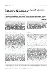
The first type of images has the obvious advantage that it does not require any specialized image processing techniques. However, its practical use in space surveillance is limited to space objects with apparent motion similar to stars. Applying the same imaging strategy to all other types of space objects by using very short exposure times reduces the sensitivity of the optical sensor. Furthermore, as mentioned above, in this case there is no way to distinguish between space objects and field stars in a single CCD frame. This results in a need to process all detections in each frame, which has a great impact on the overall computational efficiency of the imaging pipeline. The second type of imaging strategy, which implies observations with sidereal tracking, seems to have no sense at all as it also has extremely poor sensitivity of the imaging system with respect to space objects. According to this approach, the only reasonable imaging strategy in space surveillance implies tracking the target space object, if its apparent velocity is known (like in follow-up observations of a particular object), or assuming some expected velocity if it is not (like in surveytype and discovery observations). Exposure time is then chosen to be long enough to allow one to distinguish between space objects and field stars and to achieve reasonable sensitivity, but not very long to avoid producing extremely long trails of both field stars and space objects, which impacts accuracy and reliability of data reduction. As was mentioned above, techniques described here are applicable to a large class of space surveillance tasks and orbit types, when the appropriate imaging strategy is used during observations. However, this paper focuses mainly on reduction of GEO survey data obtained with wide-field optical sensors as one of the most computationally challenging problems. Figure 1 shows an example of a typical raw CCD image, one of about a thousand produced by a 22-cm aperture 5.5°×5.5° field of view optical sensor of the ISON network (Molotov et al., 2010) during a routine nightly GEO survey. One of the key requirements in space surveillance is to minimize a delay between exposure and its final result, in the form of space object coordinates. Although the overall data rate (≈8 Gigabytes of pixel data and 500–1000 tracks per night) can be considered very moderate for a modern automated imaging system, ISON sensors are installed at locations with no access to supercomputing resources and even often with very limited Internet connection. Moreover, different sensors have slightly varying characteristics and details of implementation of their parts, which affects various properties of images. All these considerations lead to very rigid requirements for data reduction software to be, on the one hand, quite efficient to be able to process data in real time and, on the other hand, sufficiently flexible and versatile to accommodate to a wide range of input data. Unfortunately, it is hard to satisfy these two requirements simultaneously: excessive optimization often makes the system less adaptable to a changing environment, while maximum flexibility entails an extra overhead of handling endless possibilities. Thus, data reduction software should elaborate a sort of compromise to be able to quickly produce a large amount of reliable data.
Apex II Pipeline for Automatic GEO object detection Apex II (Devyatkin et al., 2010) is a general-purpose platform for astronomical image processing, modeled after such well-known scientific data analysis packages as IRAF, MIDAS, IDL, and MATLAB. It is implemented mostly in Python, a high-level versatile object-oriented scripting programming language widely adopted by the scientific community. Apex II has easily extendable modular structure consisting of (i) library of astronomical data reduction algorithms and (ii) scripts (high-level interpreted programs) for specific data reduction tasks. Design of Apex II and its applications in a low-level analysis of data produced in observations of Earthorbiting objects are outlined in Kouprianov (2008). Most algorithmic details are also covered in that paper. Here we concentrate only on the most important features and latest algorithmic developments.
Us
Уд
Figure 1. Sample raw CCD image from GEO survey. Raw CCD image shown in Figure 1 displays several instrumental artifacts that need to be removed. The most obvious (and most annoying) of them is vignetting characteristic to many wide-field systems. As long as accurate CCD photometry is not required, it is sufficient to only flatten the background to allow segmentation (separation of objects from the background) by a simple global threshold; it does not matter whether the background comes from the sky or vignetting or non-uniformity of the CCD chip. Figure 2 shows the result of calibration of the same image; a fast automatic sky background estimation algorithm involved is described in (Kouprianov, 2008). The ultimate goal of the initial image processing is to detect space objects (shown enlarged in Figure 2) and accurately determine their position in terms of α and δ. To achieve this, one needs first to detect reference stars and perform astrometric reduction. Given (i) LSPC (least-squares plate constants) solution and (ii) XY positions of detected GEO objects, their αδ positions are obtained straightforwardly. αδ positions of space objects are then (iii) correlated across several adjacent images of the same sky region to obtain tracks of GEO objects and eliminate false detections. These three major stages comprise Apex II pipeline for automatic reduction of space object observations. In the following section we highlight several difficulties that arise in the astrometric reduction of CCD images from GEO surveys.
Us
Уд
Us
Уд
Us
Уд
Figure 2. Calibrated CCD image. Regions around two GEO objects are shown enlarged.
Reference Star Detection and Astrometry As was mentioned above, the characteristic feature of CCD images from GEO surveys are field stars appearing as streaks. Although this is good for detecting space objects, this apparently complicates dealing with the reference stars themselves. Things like atmospheric turbulence, extinction fluctuations, noise, and optical aberrations distort star trails. As a result, a naïve global threshold approach often fails to detect the whole trail, especially for stars close to the detection threshold, mostly due to their fragmentation. This is illustrated in Figure 3. To reduce fragmentation, we use a special kind of binary morphological filter that utilizes properties of star trail shapes known before processing: their length and orientation are easily calculated from the pixel scale, exposure duration, and tracking rate, while trail width can be estimated from the pixel scale and seeing. The following equation defines the result of filtering:
(1)
Us
Уд
where M(x,y) is the original unfiltered binary image, M′(x,y) is the filtered image, “*” denotes convolution, d is filter strength parameter, and filter kernel K is defined as follows:
Figure 3. Binary CCD image after segmentation by the global threshold: background → black, objects → white. Enlarged region containing three star trails illustrates the effect of fragmentation.
𝐾=
0 0 𝟏 0 0
0 𝟏 𝟏 𝟏 0
0 𝟏 𝟏 𝟏 0
𝟏 𝟏 𝟏 𝟏 𝟏
𝟏 𝟏 𝟏 𝟏 𝟏
𝟏 𝟏 𝟏 𝟏 𝟏
𝟏 𝟏 𝟏 𝟏 𝟏 𝟏 𝟏 ___ 𝟏 𝟏 𝟏 𝟏 𝟏 𝟏 𝟏 𝟏
𝟏 𝟏 𝟏 𝟏 𝟏
𝟏 𝟏 𝟏 𝟏 𝟏
0 𝟏 𝟏 𝟏 0
0 𝟏 𝟏 𝟏 0
0 0 𝟏 . 0 0
(2)
In other words, 1’s in the filter kernel reproduce the estimated shape of a star trail, with its length and width; if the star trail orientation differs from 0 or 180°, the kernel is rotated accordingly. The effect of the above filter is shown in Figure 4. By tuning d, one can achieve the desired balance between the number of fully detected real star streaks and the number of artifacts detected as stars. We should also mention that the global threshold for reference star detection is chosen automatically based on the image histogram. The idea behind this is quite simple: we just select such grayscale level that the number of pixels brighter than this level constitutes the fixed frac-
Us
Уд
tion of the total image area. Thus, we always get the same fraction of the image covered by reference stars, which helps to adapt to varying atmospheric conditions and stellar field densities.
Figure 4. Binary CCD image after morphological filtering for star trail enhancement: background → black, objects → white. Enlarged region is the same as in Figure 3. In the case of sources with a noticeable apparent motion in the image, it is important to clearly define which point within the streak left by the source corresponds to which exact moment of time during integration. We choose the easiest approach and assume that the visible center of streak corresponds to mid-exposure time. This has a number of implications, including those related to the times of opening and closing of the mechanical shutter and to the possible optical variability of sources (inherent or induced by atmosphere). However, this still remains the most accurate and easy to implement method for most of the real-life situations. Thus, we need to obtain XY positions of the centers of all field star trails. This is done by PSF fitting with a special type of point spread function suitable for trailed sources, as described in Kouprianov (2008). Other properties of stellar images, including their lengths, widths, and fluxes, are determined as well. Figure 5 shows a simulated image with real field stars approximated by their ideal models obtained by PSF fitting. One may observe a number of artifacts there – mostly caused by the overlapping of multiple star streaks. The latter is very difficult to handle, which imposes two important restrictions on observations: (i) exposure time should not be too long to reduce the length of streaks and (ii) one should avoid rich stellar fields in the Milky Way. This also reduces the
Us О По
Us
Уд
Us
Уд
probability of overlapping with space objects, which is critical for the reliability of their detection.
Figure 5. Simulation image of reference stars. When PSF fitting is complete, several criteria are applied to eliminate false and unreliable detections. Most important of them are the constraints on full width at half maximum (FWHM) across the trail, and on the deviation of the measured length and orientation of the trail from that expected. Stars that pass these criteria undergo the classical differential astrometric reduction sequence that includes matching against a reference catalog and obtaining a LSPC solution by fitting a parameterized plate model that maps XY catalog positions to measured XY positions of the reference stars (see e.g. Green, 1985). For large fields of view common to survey cameras Tycho–2 (Høg et al., 2000) is the catalog of choice; however, for instruments with fields of view less than about 1°, UCAC3 (Zacharias et al., 2009) appears to be also suitable. Apex II has a number of predefined plate models, both linear and non-linear in parameters. An important issue with wide-field optical systems is the presence of residual optical aberrations, especially at image corners, that need to be eliminated to achieve accurate astrometry across the whole field of view. From the point of view of differential astrometry, any optical aberration can be treated as generalized distortion, i.e. a systematic displacement of centroids of stars; then, if we have enough reference stars, distortion parameters are obtained just as any other plate constants. An example of such model is a simple cubic model with all terms:
Figure 6. Example of optical distortions of a typical ISON survey camera. Displacement vectors are enlarged by factor 20. ! !"!! ! ! ! !! ! ! ! !! ! ! ! !!! ! !! ! !! ! ! ! , ! ! !!!!"!!"!! !! ! ! !!!" ! !! !! !! ! !!! !! !
!
!
!
!
!
!
! ! !!!!"!!"!! ! ! ! !!!" !"!! ! ! ! !! ! ! ! !! ! ! ! !!! ! !! ! !! ! ! ! , ! ! ! ! ! !! !
(3)
where x and y are catalog positions, while x′ and y′ are measured positions. Another one (Brown, 1966) is suitable for handling pure radial and tangential distortions: ! ! !!!!"!!"!!! ! ! !!!! ! ! !!!! ! ! !!! ! !!! !", ! ! !!!!"!!"!!! ! ! !!!! ! ! !!!! ! ! !!! ! !!! !",
(4)
where r2 = x2 + y2. However, when optical distortions become extremely large, even choosing the appropriate plate model might appear insufficient. Due to very large deviations of actual reference star positions from their expected positions, especially at the peripheral parts of image, the catalog matching algorithm may fail with such stars, so they won’t be included in the final LSPC solution. This will result in systematic errors at image edges. An example of an image with strong optical distortions is shown in Figure 6. The solution is to perform all the astrometric reduction steps several times, with more and more peripheral stars being included at each iteration as the LSPC solution becomes more and more reliable over the whole field of view. This technique leads to excellent accuracy, even in the presence of strong distortions, provided the plate model is adequately chosen. As a real-life example we would mention the pure positional accuracy of about 0.1″ along each axis for a pixel scale of 10″/ pixel that is achieved in good atmospheric conditions.
Us
Уд
GEO Object Detection As one can see from Figure 4, space objects may become apparent even in the course of reference star detection, so, at first glance, there is no need for a separate space object detection
Us
Уд
Figure 7. Effect of morphological filter (5), (6) on a fragment of binary image containing star trails and a single GEO object. Left: before filtering; right: after filtering. step. Unfortunately, this is the case only for bright point-like objects. Fainter objects, as well as those having considerable apparent motion directed across the diurnal motion of stars, are wiped out by the star trail enhancement filter. Moreover, for better computational performance, the global threshold for reference star detection is chosen comparatively high to take only as many stars as needed for accurate astrometry, so we merely loose faint space objects. Therefore, it is necessary to establish a separate space object detection stage, with as low a detection threshold as possible (in practice, we use thresholds of down to 2.5σ, where σ is the noise level). Of course, such low threshold values would result in large amounts of false detections (here a field star is also considered a “false detection”). Fully processing all these detections to determine whether they are false or not would be impractical from the computational point of view. Hence, we need to work out a process that quickly eliminates most of the false detections, including stars, as early as possible, leaving space objects intact. Here the morphological difference between space objects and stars comes into play. One of the possible ways to remove groups of pixels left by star trails is to use a technique similar to that described in the previous section, but acting in the opposite direction. The filtering operator is now defined as
(5) Note that “>” in (1) is replaced by “