Apr 4, 2012 - we identify all relevant terms in TAs: (i) In the limit. â â 0, the TA ... the distribution Ï(t) of waiting times all TAs of physical .... USA 108, 6438.
Ageing effects in single particle trajectory averages Johannes Schulz,1 Eli Barkai,2 and Ralf Metzler3, 4 1
arXiv:1204.0878v1 [cond-mat.stat-mech] 4 Apr 2012
Physics Department T30g, Technical University of Munich, 85747 Garching, Germany 2 Department of Physics, Bar Ilan University, Ramat-Gan 52900, Israel 3 Institute for Physics & Astronomy, University of Potsdam, 14476 Potsdam-Golm, Germany 4 Physics Department, Tampere University of Technology, FI-33101 Tampere, Finland (Dated: 5th April 2012) We study time averages of single particle trajectories in scale free anomalous diffusion processes, in which the measurement starts at some time ta > 0 after initiation of the process at the time origin, t = 0. Using ageing renewal theory we show that for such non-stationary processes a large class of observables are affected by a unique ageing function, which is independent of boundary conditions or the external forces. We quantify the weakly non-ergodic nature of this process in terms of the distribution of time averages and the ergodicity breaking parameter which both explicitly depend on the ageing time ta . Consequences for the interpretation of single particle tracking data are discussed. PACS numbers: 87.10.Mn,02.50.-r,05.40.-a,05.10.Gg
Ergodicity in the Boltzmann sense, the equivalence of sufficiently long time and ensemble averages of a physical observable, and time translational invariance are hallmarks of many classical systems. In contrast, ergodicity violation and ageing effects are found in the dynamics of various complex systems including glasses [1], blinking quantum dots [2], weakly chaotic maps [3], and single particle tracking experiments in living biological cells [4]. As originally pointed out by Bouchaud [1], when the lifetimes t of states of a physical system are power-law distributed, ψ(t) ≃ τ α /t1+α (0 < α < 1), with an infinite mean sojourn time hti, both weak ergodicity breaking and ageing in the following sense occur: time averages of physical observables remain random even in the limit of long measurement times and differ from the corresponding ensemble averages [5–14]. Furthermore ensemble averaged correlation functions of observables, taken at two time instants t2 and t1 , are not solely functions of the time difference |t2 − t1 |. With this breakdown of stationarity, the statistical properties of such systems are no longer time translation invariant. Consider, for example, a particle undergoing a random walk in a random environment, such that the particle hops a finite distance to the left or right with equal probability, but sojourn times between jumps are distributed like ψ(t). Such a model, called the continuous time random walk model (CTRW), was introduced by Scher and Montroll in the context of charge carriers in disordered systems [15]. Its intriguing statistical properties become apparent when studying time averages, like the time averaged mean squared displacement (TAMSD), which is commonly used to analyze the diffusive properties measured in single particle tracking assays. Assume that the process starts at time t = 0. From a single trajectory x(t), observed in the time interval (ta , ta + T ), the TAMSD is typically determined through the definition Z ta +T −∆ 2 [x(t + ∆) − x(t)] 2 dt, (1) δ (∆; ta , T ) = T −∆ ta
with the lag time ∆ and the measurement time T . For Brownian motion, in the limit of large T , we obtain the expected behavior, namely, δ 2 → 2K1 ∆. In this case, the process does not age: the result does not depend on the choice of ta . Moreover Brownian motion is ergodic: the result for the TAMSD is not random, and the same as found for an ensemble of Brownian particles, hx2 (∆)i = 2K1 ∆ [16]. Thus the diffusion constant K1 can be determined either from an ensemble of trajectories as originally done by Perrin [17] or, as conceived by Nordlund [18], from a single particle trajectory. For anomalous diffusion, defined in terms of hx2 (∆)i = 2Kα ∆α /Γ(1 + α) with the generalized diffusion constant Kα , the equivalence between time and ensemble averages as well as the time translation invariance generally breaks down. One of our central results is that for CTRW processes with long tailed ψ(t) the aged TAMSD (1) for ∆ ≪ T follows D
E Λ (t /T ) g(∆) α a δ 2 (∆; ta , T ) = , Γ(1 + α) T 1−α
(2)
where Λα (z) = (1 + z)α − z α , and g is a function of ∆ only. Another important finding is that δ 2 remains a random variable, whose statistical properties explicitly depend on both process age ta and measurement time T . Previous work revealed deviations from standard ergodic statistical mechanics by studying time averages in the interval (ta = 0, T ) [6–12]. Namely, in these works the start of the measurement coincides with the start of the process [19]. However, in experiment, the observed particle may be immersed in the medium long before we start our observation. In fact in some cases we may not even know when the process was initiated. In this Letter, we derive the ageing renewal theory for CTRW processes and study the dependence of time averages of physical observables on the starting time ta of a measurement after system preparation at t = 0. According to Eq. (2), the time intervals (0, T ) and (ta , ta + T )
2 are not equivalent: In complete contrast to Brownian motion, the statistical properties of CTRW trajectories will depend on the observation window, the process exhibits ageing. The remarkable property of Eq. (2) is that corrections due to ageing enter in terms of a unique prefactor depending on ta and the measurement time T . We call this Λα the ageing depression function, which is independent of ∆. This function contains all the information on ageing, and is universal since the formula applies for any external force or boundary condition, and, as shown below, also holds for a large class of physical observables. The function g(∆) contains the complete ∆-dependence. For instance, we find g(∆) ≃ ∆ for free motion [6, 7] and g(∆) ≃ ∆1−α at long times under confinement [9, 10]. Ageing renewal theory. In a CTRW, the position coordinate x of a random walker Pisn an accumulation of random jump lengths, x(n) = i=0 δxi . In the simplest, unbiased version of the model, the δxi are independent, identically distributed (IID) random variables with zero mean, and we assume also finite variance σ 2 . Jumps are separated by random IID waiting times, drawn from the common distribution ψ(t) ≃ τ α /t1+α , with 0 < α < 1. This implicitly defines a counting process n(t), the number of steps up to time t. The statistics of the overall diffusion process x(t) = x(n(t)) are to be derived from the properties of both of its constituents, a method commonly called subordination [20–22]. For a large variety of physical applications of CTRW and non-aged renewal theory see [15, 23, 24]. We first discuss the counting process n(t), emphasizing the role of ageing. Since waiting times are independent, the counting process n(t) is a renewal process, which we assume to start at t = 0. To study the ageing properties of the system, we consider na (ta , t) = n(t+ta )−n(ta ), the number of renewals in the interval (ta , ta +t). The corresponding probability density in double Laplace space, (ta , t) → (sa , s), in the scaling limit of large times becomes [25, 26] � � α h(sa , s) h(sa , s) 1 + 1−α τ α e−na (sτ ) . − p(na ; sa , s) = δ(na ) sa s s s (3) Here the probability of the waiting time for the first jump to occur after start of the measurement at ta is [26–28] sα − sα tα h(sa , s) = α a ⇔ h(ta , t) = α a . sa (sa − s) t (ta + t)
(4)
= Γ(q + 1)
α τα sα a −s . 1+αq sα a (sa − s) s
hnqa (ta , t)i = Γ(q + 1)/ [Γ(α)Γ(1 + αq − α)] �αq � � � t t + ta B ; 1 + αq − α, α , × τ t + ta
(5)
(6)
where B(z; a, b) is the incomplete beta function [30]. Thus, the number of steps taken during a time interval of length t is not stationary in distribution: the moments for the period [0, t] are clearly different from those for [ta , ta + t]. Indeed we see from Eqs. (5) and (6) that the process gets slower and eventually stalls as ta → ∞. Concurrently the t-dependence changes with ta : hnqa (0, t)i ≃ tαq at ta = 0, but hnqa (ta , t)i ≃ tα−1 t1−α+αq a for large but finite ta /t. For the probability density (3) we obtain p(na ; ta , t) ∼ [1 − mα (t/ta )] δ(na ) + mα (t/ta )Γ(2 − α) � � 1 na (2 − 2α, α) 1,0 × H (7) (t/τ )α 1,1 (t/τ )α (0, 1)
for ta ≫ t, in terms of an H-function [31, 32] and the probability to make at least one step during [ta , ta + t], � B [1 + ta /t]−1 , 1 − α, α mα (t/ta ) = . (8) Γ(1 − α)Γ(α) Again, we emphasize the explicit dependence on ta . When compared to the form for ta = 0 [6, 27], the most striking difference in Eq. (7) is the occurrence of the δ(na )-term: For a non-aged process (ta = 0), we have mα = 1, while an aged process always has a nonzero probability of not performing any steps at all within the chosen time window, its amplitude approaching 1 algebraically, mα ∼ (t/ta )1−α /[Γ(α)Γ(2 − α)], as ta ≫ t. Ageing CTRW. We proceed by adding the position coordinate to our description. For IID jump distances δxi , the jump process x(n) converges in distribution to free Brownian motion in the scaling limit of many jumps. The anomalous diffusion process x(t) = x(n(t)) inherits the ageing properties of the counting process discussed above. To see this, consider the qth order TA moments E Z ta +T −∆ h|x(t + ∆) − x(t)|q i D q δ (∆; ta , T ) = dt, (9) T −∆ ta which are useful to characterize experimental data [33]. For free Brownian motion x(n) we know that h|x(n2 ) − x(n1 )|q i =
In the Brownian limit α → 1, the number of jumps n and real time t are equivalent, p(na ; ta , t) = δ(na − t/τ ). This formalism allows for a direct calculation of the average of any function of na (ta , t). For instance, the qth order moment becomes [29] Z ∞ hnqa (sa , s)i = nqa p(na ; sa , s) dna 0
After double Laplace inversion, we find
2Γ(q) σ q |n2 − n1 |q/2 , Γ(q/2) 2q/2
(10)
Since x(n) and n(t) are independent processes, we use conditional averaging to evaluate the integrand of Eq. (9). From above result (6), it follows that 2Γ(q) σ q hnq/2 (t, ∆)i Γ(q/2) 2q/2 a = Γ(q + 1)/ [Γ(α)Γ(1 + αq/2 − α)] � � ∆ α q/2 , 1 − α + αq/2, α ,(11) × [Kα (t + ∆) ] B t+∆ q
h|x(t + ∆) − x(t)| i =
3
δ2
mα=1
−1
10
δ2
−1
10
−3
10
−5
10 −1 10
mα=0.063
quantities will be provided below. The result reads D
−3
10
−5
0
10
∆
1
10
10 −1 10
0
10
∆
1
10
Figure 1: Time averaged mean squared displacement δ 2 (∆; ta , T ) for individual free CTRW trajectories (full symbols) and the averages according to Eq. (12) (bold black lines). Left: Measurement starts at ta = 0, so that mα = 1. Right: Aged process, ta = 1011 (a.u.), so that a large fraction 1 − mα ≈ 94% of trajectories is suppressed in the log-log plot. The parameters are α = 1/2, τ = 1, σ 2 = 1 and T = 109 .
where we identify Kα = σ 2 /(2τ α ) [23]. The qth order TA moment (9) in the limit ∆ ≪ T then becomes E Λ (t /T ) [K ∆α ]q/2 Γ(q + 1) � ∆ �1−α α a α , a, T ) = Γ(α + 1)Γ(2 − α + αq/2) T (12) which is of the general shape (2) with g(∆) ∼ ∆1−α+αq/2 . Interestingly, we see the special role of the TAMSD (q = 2), for which the ∆-scaling is independent of α. Fig. 1 shows simulations results for the TAMSD. If evaluated during the initial time period, ta = 0, the TAMSD for individual trajectories scatter around the ensemble average hδ 2 i, Eq. (12). In contrast, for the aged process (ta ≫ T ) the ensemble average hδ 2 i appears much lower than the shown individual trajectories. This is due to the fact that a significant fraction 1 − mα of particles do not move during the entire measurement time. Such trajectories are naturally not visible in a logarithmic plot, while being included in the calculation of hδ 2 i. In a biological cell, the diffusive motion of a tracer particle is spatially confined, or a charge carrier in a disordered semiconductor experiences a drift force. To address such systems we now determine the TAMSD in the presence of an external potential. We start with a Hookean force −λx and address the more general case below. To that end the continuum approximation of the process is represented by the Langevin equation [34] D
δ q (∆; t
dx/dn = −λx(n) + ξ(n),
(13)
where ξ(n) is white Gaussian noise with hξ(n1 )ξ(n2 )i = σ 2 δ(n2 − n1 ). In other words, x(n) is a stationary Ornstein-Uhlenbeck process. Its increments are Gaussian variables, characterized by the variance h[x(n2 ) − x(n1 )]2 i = σ 2 [1 − exp(−λ|n2 − n1 |)]/λ. To calculate the TAMSD, we follow the approach outlined for the free particle, a general approach to compute this and similar
E Λ (t /T ) 2K ∆ α α a δ 2 (∆; ta , T ) = Eα,2 (−λα ∆α ) (14) Γ(1 + α) T 1−α
in terms of the generalized Mittag-Leffler function [35], where λα = λ/τ α . We deduce the limiting behavior ( −1/α D E 2Λ (t /T )K ∆, ∆ ≪ λα α a α 2 1−α δ ∼ −1/α . (15) ∆ /λα Γ(1 + α)T 1−α Γ(2−α) , ∆ ≫ λα Eq. (14) is another special case of Eq. (2). Interestingly the entire dynamics are multiplied by the unique factor Λα . Let us now test the generality of this feature. Consider the time average of some observable F (x2 , x1 ) along the trajectory, E Z ta +T −∆ hF (x(t + ∆), x(t))i D F (∆; ta , T ) = dt. (16) T −∆ ta F may represent moments (F = δ q , F (x2 , x1 ) = |x2 − x1 |q ) or the TA of a correlation function. We only require that the jump process x(n) and the function F fulfill hF (x(n2 ), x(n1 ))i = f (n2 − n1 ).
(17)
For instance, we have f (n) = σ 2 n for the second moment of unbounded motion [cf. (10)], or f (n) = σ 2 [1 − exp(−λn)]/λ for the TAMSD in an harmonic potential. Condition (17) is fulfilled whenever x(n) is a stationary process (e.g., equilibrated Brownian motion). Alternatively, one may consider a process with stationary increments (e.g., unbounded Brownian motion), when F (x2 , x1 ) = F (x2 − x1 ). In these cases we find ta +T −∆
f (na )p(na ; t, ∆) dna dt, T −∆ ta 0 (18) where p(na ; ta , t) is defined in Eq. (3). We obtain D
E Z F (∆; ta , T ) =
D
Z
∞
E Λα (ta /T ) g(∆/τ ) , F (∆; ta , T ) = C + Γ(1 + α) (T /τ )1−α
(19)
at short lag times ∆ ≪ T , with the constant C = f (0). The function g in Laplace space is defined as [25] g(s) = s2α−2 L {f (n) − f (0); n → sα } .
(20)
Comparing with our specific results (2), (12), and (15), we identify all relevant terms in TAs: (i) In the limit ∆ → 0, the TA reduces to the constant C, which equals the expectation value of the observable when measured at identical positions. For example, if we study correlations in an equilibrated process, F (x2 , x1 ) = x2 x1 , then C = hx2 i is the thermal value of x2 . Conversely, C naturally vanishes if we are interested in TA moments of displacements, F (x2 , x1 ) = |x2 − x1 |q , so it did not appear previously. (ii) The lag time dependence enters
4 1
10
free
non-aged in a box
0
10
aged free
0.8
0.04
0.6
0.03
0.4
0.02
0.2
0.01
in a box 0
0
0
1
2
3
4
0
5
10
15
20
−1
10
−1
0
10
1
10
10
Figure 2: Numerical validation of Eq. (21), for various α, boundary conditions, and ta (see key). Each point in the graph represents an individual trajectory. Parameters are τ = 1 (a.u.), σ 2 = 1, ∆ = 100, T = 2 × 10⁶ . ta is either 0 (nonaged), or for specific α chosen such that mα = 0.054 (aged).
Figure 3: Scatter density φ(ξ) for different α and mα , see text. Lines: Eq. (7) from [6] (Left) and Eq. (22) (Right). Symbols: Simulations of free CTRW. Note that the area under the curves for the aged process in the right panel is not unity, since the fraction 1 − mα of immobile events is not shown. Same parameters as in Fig. 2. 2
10
4
3
through the function g(∆). For example, if f (n) ∼ nq , then C = 0, and in Laplace space g(s) ∼ sα−2−αq , which implies g(∆) ∼ ∆1−α+αq as in Eq. (12). (iii) The ageing depression function Λα only depends on the ratio ta /T and the parameter α, and due to a factor T α−1 any TA converges to the constant C as T → ∞. Note that this dependence on ageing and measurement time ta and T is universal in the sense that it is indifferent to the specific choice of observable F or model of the jump process x(n), but is directly deduced from the nature of the ageing counting process n(t). Also note that in the Brownian limit α = 1, Eq. (19) reduces to hF (∆; ta , T )i = f (∆/τ ), restoring the ergodic equivalence of ensemble and time averages, and the stationarity of the process. Distribution of TAMSD. Due to the scale-free nature of the distribution ψ(t) of waiting times all TAs of physical observables, e.g. δ 2 , remain random quantities, however, with a limiting distribution φ(ξ) for the dimensionless ratio ξ = δ 2 /hδ 2 i [6, 10, 36]. As contributions to time averages of the form (1) occur at time instants when the particle performs a jump, we expect that in the sense of d distributions both δ 2 and na should be equivalent, δ 2 = cna , for some non-random, positive c. In other words, ξ=
δ 2 (∆; ta , T ) hδ 2 (∆; t
a , T )i
d
=
na (ta , T ) , hna (ta , T )i
(21)
for ∆ ≪ T . We may thus deduce the statistics directly from the underlying counting process. Fig. 2 provides numerical evidence for this argument in the case of a free particle and a particle in a box for several values of α. The distribution φ(ξ) for ta = 0 is related to a onesided L´evy stable law [6]. In the opposite case ta ≫ T , combination of Eqs. (21) and (7), yields φ(ξ) ∼ [1 − mα (T /ta )] δ(ξ) + mα (T /ta )Γ(2 − α) � � 1−α (T /ta )1−α (2 − 2α, α) (T /ta ) 1,0 H1,1 ξ , (22) × Γ(α) Γ(α) (0, 1)
1
10
2 0
10 1
−1
0 0
10 0.2
0.4
0.6
0.8
1
−2
10
−1
10
0
10
1
10
2
10
3
10
Figure 4: Ergodicity breaking parameter (23) as function of α (Left) and ta /T (Right). Notice that the non-ergodic fluctuations become larger with increasing ta .
for ∆ ≪ T ≪ ta . In φ(ξ), mα (T /ta ) is the weight of the continuous part. The probability for not moving during the whole measurement period, (ξ = 0), approaches unity as ≃ (T /ta )1−α . If conditioned to measurements with ξ > 0, we also find the scaling ξ ∼ (ta /T )1−α . In Fig. 3 we demonstrate excellent agreement of Eq. (22) with numerical simulations. Deviations from ergodic behavior are quantified by the ergodicity breaking parameter [6], for which we obtain D 2E � δ2 B [1 + ta /T ]−1 , 1 + α, α − 1, EB = D E2 − 1 = 2α [1 − (1 + T /ta )−α ]2 δ2 (23) depending only on the ratio ta /T . At ta = 0 EB reduces to the result of Ref. [6], while for ta ≫ T , we find EB ∼ 2(ta /T )1−α /[α(1 + α)]. In the non-aged case EB is bounded, 0 ≤ EB ≤ 1, depending on the value of α only. In contrast we find that EB may diverge in the limit ta /T → ∞. This implies that the non ergodic fluctuations are much larger in the aged regime under investigation. We show the behavior of EB in Fig. 4. Conclusions. We investigated the effects of ageing on TAs of physical observables. Previous calculations of TAs tacitly neglect the fact that often the preparation of the system and start of the measurement do not coincide.
5 While this does not cause any problems for ergodic systems with rapid memory loss of the initial conditions, in general this cannot be taken for granted in processes of anomalous diffusion. Here we showed for the case of CTRW with diverging characteristic waiting time that TAs of arbitrary physical observables carry the common factor Λα . This ageing depression function is universal in the sense that it only depends on the process age ta and the measurement time T . All details such as confinement effects enter through a single function, g(∆). The structure of this result was shown to hold for a large class of physical observables. We also see that the ageing of the process has a pronounced statistical effect, splitting the population into two: the mobile fraction mα and the immobile one whose amplitude 1 − mα grows with ta /T . Knowledge of this effect is significant for the quantitative physical interpretation of experimental data. Finally, since renewal theory is applicable to many systems, our results with minor changes should be relevant more generally, for instance, to the Aaronson-DarlingKac theorem in infinite ergodic theory or for counting the number of renewals in blinking quantum dots. We acknowledge funding from the CompInt graduate school, the Academy of Finland (FiDiPro scheme), and the Israel Science Foundation.
[1] J.-P. Bouchaud, J. Phys. I (Paris) 2, 1705 (1992). [2] F. D. Stefani, J. P. Hoogenboom, and E. Barkai, Phys. Today 62(2), 34 (2009). [3] N. Korabel and E. Barkai, Phys. Rev. Lett. 102, 050601 (2009); ibid. 108, 060604 (2012). [4] J.-H. Jeon et al., Phys. Rev. Lett. 106, 048103 (2011); A. V. Weigel et al., Proc. Nat. Acad. Sci. USA 108, 6438 (2011). [5] G. Bel and E. Barkai, Phys. Rev. Lett. 94, 240602 (2005); A. Rebenshtok and E. Barkai, ibid. 99, 210601 (2077). [6] Y. He, S. Burov, R. Metzler, and E. Barkai, Phys. Rev. Lett. 101, 058101 (2008). [7] A. Lubelski, I. M. Sokolov, and J. Klafter, Phys. Rev. Lett. 100, 250602 (2008). [8] W. Deng and E. Barkai, Phys. Rev. E 79, 011112 (2009); J.-H. Jeon and R. Metzler, ibid. 81, 021103 (2010); ibid. 85, 021147 (2012). [9] T. Neusius, I. M. Sokolov, and J. C. Smith, Phys. Rev. E 80, 011109 (2009) [10] S. Burov, J.-H. Jeon, R. Metzler, and E. Barkai, Phys. Chem. Chem. Phys. 13, 1800 (2011); S. Burov, R. Metzler, and E. Barkai, Proc. Natl. Acad. Sci. USA 107, 13228 (2010).
[11] T. Akimoto et al., Phys. Rev. Lett. 107, 178103 (2011). [12] I. M. Sokolov, E. Heinsalu, P. H¨ anggi, and I. Goychuk, EPL 86, 30009 (2009). [13] M. A. Lomholt, I. M. Zaid, and R. Metzler, Phys. Rev. Lett. 98, 200603 (2007); I. M. Zaid, M. A. Lomholt, and R. Metzler, Biophys. J. 97, 710 (2009). [14] D. Boyer, D. S. Dean, C. Mej´ıa-Monasterio, and G. Oshanin, Phys. Rev. E 85, 031136 (2012). [15] H. Scher and E. W. Montroll, Phys. Rev. B 12, 2455 (1975). R∞ [16] In the sense that hx2 (t)i = −∞ x2 P (x, t)dx, where P (x, t) is the probability density function of the process. [17] J. Perrin, Compt. Rend. (Paris) 146, 967 (1908); Ann. Chim. Phys. 18, 5 (1909). [18] I. Nordlund, Zeit. Phys. Chem. 87, 40 (1914). [19] Note that in some cases the start of the measurement and the start of the process coincide. For example, in the original work of Scher and Montroll [15], a light flash excites charge carriers in a disordered semiconductor. Similarly, in a glassy system we may suddenly quench the temperature, thus defining physically the start of the process. [20] H. C. Fogedby, Phys. Rev. E 50, 1657 (1994). [21] A. Baule and R. Friedrich, Phys. Rev. E 71, 026101 (2005). [22] M. Magdziarz, A. Weron, and K. Weron, Phys. Rev. E 75, 016708 (2007). [23] R. Metzler and J. Klafter, Phys. Rep. 339, 1 (2000); J. Phys. A 37, R161 (2004). [24] X. Brokman et al., Phys. Rev. Lett. 90, 120601 (2003); G. Margolin and E. Barkai, ibid. 94, 080601 (2005). [25] We express R ∞ the Laplace transform f (s) = L {f (t); t → s} = 0 f (t) exp(−st)dt of a function f (t) by explicit dependence on the Laplace variable s. [26] E. Barkai, Phys. Rev. Lett. 90, 104101 (2003); E. Barkai and Y.-C. Cheng, J. Chem. Phys. 118, 167 (2003). [27] T. Koren et al., Phys. Rev. Lett. 99, 160602 (2007). [28] C. Godr`eche and J.M. Luck, J. Stat. Phys. 104, 489 (2001). [29] J. Schulz, E. Barkai, and R. Metzler (unpublished). [30] M. Abramowitz and I. Stegun, Handbook of Mathematical Functions (Dover, New York, 1971). [31] A. M. Mathai, R. K. Saxena, and H. J. Haubold, The H-Function, Theory and Applications, Springer (2009) [32] The H-function admits series expansions for small and large arguments which we used to plot the curves in Fig. 3. [33] V. Tejedor et al., Biophys. J. 98, 1364 (2010). [34] C. W. Gardiner, Handbook of stochastic methods for physics, chemistry, and the natural sciences (Springer, Berlin, 1989). [35] A. Erd´elyi, Higher Transcendental Functions, Vol. 1, Bateman Manuscript Series Project (Mc-Graw Hill, New York, 1954). [36] J.-H. Jeon and R. Metzler, J. Phys. A 43, 252001 (2010).