chaotic Ikeda map [13], and the real-world Abalone,. Boston Housing, Ozone and Servo databases[14]. In the case of the Friedman#1 data set we can control the ...
Aggregation Algorithms for Neural Network Ensemble Construction P. M. Granitto, P. F. Verdes, H. D. Navone, H. A. Ceccatto Instituto de Física Rosario, CONICET-UNR, Boulevard 27 de Febrero 210 Bis, 2000 Rosario, República Argentina {granitto; verdes; navone; ceccatto}@ifir.edu.ar Abstract How to generate and aggregate base learners to have optimal ensemble generalization capabilities is an important questions in building composite regression/classification machines. We present here an evaluation of several algorithms for artificial neural networks aggregation in the regression settings, including new proposals and comparing them with standard methods in the literature. We also discuss a potential problem with sequential algorithms: the non-frequent but damaging selection through their heuristics of particularly bad ensemble members. We show that one can cope with this problem by allowing individual weighting of aggregate members. Our algorithms and their weighted modifications are favorably tested against other methods in the literature, producing a performance improvement on the standard statistical databases used as benchmarks.
1. Introduction Good regression/classification ensemble members must be both accurate and diverse. A common way of balancing these two conflicting conditions is training the base learners on different subsets of the data set. The chance of success in this strategy is directly tied to the instability of the learning algorithm (sensitiveness to small changes in the structure of the data and/or parameters defining the learning process) [1]. Artificial neural networks (ANNs), on which we will focus here, are a classical example in this sense [2]. Their instability comes naturally from the inherent data and training process randomness, and also from the intrinsic nonidentifiability of the model. The combination of strong instability of the learning algorithm with the trade-off predictors’ diversity vs. good individual generalization capabilities requires an adequate selection of the ensemble members. Attempts to achieve a good compromise between these properties include elaborations of two general techniques: bagging [1] and boosting [3,4]. Bagging (short for ‘bootstrap aggregation’), and variants thereof, train independent
predictors on bootstrap re-samples of the available data, employing the unused examples for validation purposes. These predictors are then aggregated according to different rules (most often simple or weighted average). Boosting and its variants are stagewise procedures that, starting from a predictor trained on the original data set, sequentially train new aggregate members on bootstrap re-samples drawn with modified probabilities. Each example is given a different chance to appear in a new training set by prioritizing patterns poorly learnt on previous stages. In the end, the predictions of the different members so generated are weighted with a decreasing function of the mean error each predictor makes on the available data. For regression problems, which are our main concern here, boosting is still a construction area [5-7]. Consequently, bagging is the most common method for ANN aggregation. On the other hand, intermediate alternatives between bagging and boosting, which optimize directly the ensemble generalization performance instead of seeking for the best individual members, have not been much explored yet [8-10]. In this work we discuss different strategies for ensemble construction, restricting ourselves to the following two conditions: i) as stated before, we work in the regression setting using ANNs as base learners, and, ii) we consider only strategies that allow the independent, parallel training of ANNs. The first restriction is not essential; in principle, our analysis can be extended to classification problems and to other suitable regression/classification methods. The second condition leaves out boosting-type strategies, since these require the sequential training of networks because of the modification of bootstrap re-sampling probabilities. Allowing the parallel training of networks can be very convenient when using computer clusters as in our case. Furthermore, we will discuss stepwise algorithms to select the best aggregate after network training, thus incorporating the condition of optimal ensemble performance. Our aim is to compare several alternatives for ANN ensemble construction, some of them already proposed in the literature and others first presented here, in order to establish rules as general as possible to efficiently build regression aggregates.
The organization of this work is the following: In Section 2 we briefly recapitulate simple methods proposed in the literature to aggregate regressors and present new algorithms for this task. In Section 3 we obtain empirical evidence of their relative efficiency by applying these methods to several synthetic and realworld databases. Then, in Section 4 we present a modified, weighted version of the different algorithms and test their performances using the same databases. Finally, in Section 5 we summarize and draw some conclusion.
2. Ensemble Construction Algorithms The simplest way of generating a regressor aggregate is bagging [1]. According to this method, from the data set D containing N examples one generates bootstrap resamples Ti (i=1,M) by drawing with replacement �N training patterns. The remaining examples in Vi = D i are generally used for validation purposes in the regressor learning phase (backpropagation training of the ANN in our case). In this way one generates M different members fi of the ensemble, whose ouputs on a test point x are finally averaged to produce the aggregate prediction Φ(x) = w1f1(x) + ... + wM fM(x). The normalized weights wi are usually taken equal to 1/M. Notice that according to this method all the regressors are trained independently and their performances individually optimized using the hold-out data in Vi. Then, although there is no fine-tuning of the ensemble members, the method frequently improves largely on the average performance of the single regressors fi. A slightly more sophisticated algorithm follows the same steps indicated for bagging, except that the regressors are not optimized individually but as part of the aggregate. For ANNs, the simplest way to do this is to keep a fraction of the dataset D unseen by all the networks during their training phases, and chosing the (common) optimal number of training epochs for all networks by optimizing the ensemble performance on this set [11]. However, in the common situation of scarcity of data, the need to keep an independent validation set is a serious drawback that limits the efficacy of this method. An alternative approach is to resort to the patterns (tp,xp)∈Vi unseen by network fi (i=1,M), and optimize with respect to the number of training epochs the error Err(τ) = ∑p=1,N [tp - Φ(xp,w(τ))]2 . Here w(τ) are the internal parameters (weights and biases) at epoch τ, and Φ(xp,w(τ)) = ∑i=1,M wi[xp] fi [xp,w(τ)] is the aggregate regressor built with those networks that have not seen pattern (tp,xp) in their training phase, i.e., wi[xp] = γip / ∑i γip, where γip = 1 if (tp,xp)∈Vi and 0 otherwise. Thus, the algorithm selects a common optimal
stopping point τopt for all the networks in the ensemble by minimizing the ensemble generalization error, instead of validating the ensemble members one by one over the sets Vi to maximize their individual performances as in bagging. In practice one finds that τopt is in general larger than the individual stopping points found in bagging, i.e., some controlled degree of overfitting improves the aggregate performance. In the following we will refer to this algorithm as “Epoch”. The above described strategy can be further pushed on by selecting not a single optimal number of epochs τopt for all networks but independent τiopt for each network in the ensemble. This is the proposal of the so-called NeuralBAG algorithm [12], which minimizes Erri (τ) = ∑ (t,x) ∈Vi [t - Φ i(x,w(τ))]2 to select τiopt . This is a rather ad hoc criterion (notice that the networks fk with k≠i are trained up to τiopt in the aggregate Φ i, but they are trained τkopt epochs in the final ensemble); nevertheless, it seems to be very effective in practice. Notice also that in this case one is forced to store all the intermediate networks fi [w(τ)], although in most applications this requirement is not severe. Here we propose a better strategy consisting in effectively minimizing Err(ττ) = ∑p=1,N [tp - Φ(xp,w(ττ))]2 as a function of the set of training epochs τ={τi ; i=1,M} corresponding to each network. This can be accomplished, for instance, by using simulated annealing in τ-space. That is, starting from networks trained τ0 epochs, we randomly change τ0i and check whether the ensemble generalization error increases or decreases when network i is trained up to τ0i+∆τ. This is repeated many times while reducing the annealing temperature, accepting or rejecting the moves with the standard probabilities until Err(ττ) settles in a deep local minimum. This algorithm will be called “SimAnn”. All the strategies for ANN aggregation discussed so far minimize, in a global way, some particular error function. A different approach is to generate an ANN ensemble through the sequential aggregation of individual predictors, where the learning process of a new ensemble member is validated by the previous-stage aggregate prediction performance [9,10]. That is, the early-stopping method is applied by monitoring the generalization capability of the n-stage aggregate predictor plus the n+1 network being currently trained on the validation data set Vn+1. In this way one retains the simplicity of independent network training and only the validation process becomes slightly more involved, leading again to a controlled overtraining (“late-stopping”) of the individual networks. Notice that, despite the stepwise characteristic of this
some of the other algorithms described before. In the next section we will investigate how the different heuristics outlined in this section work on real and synthetic data.
algorithm (called SECA, for Stepwise Ensemble Construction Algorithm), it can be implemented after the parallel training of networks if desirable. Alternatively, if implemented sequentially it avoids completely the burden of storing networks at intermediate training times like in -2
Table 1. Normalized mean-squared test errors (in units of 10 ). Upper table: Friedman #1 data set. Lower table: Databases indicated. The results for Single correspond to the average performance of a single ANN. The best result in each case is highlighted in bold.
Noise & Length 50 Free 100 200 50 Low 100 200 50 High 100 200 Database Abalone Boston Ozone Servo Ikeda
Single 4.53 3.39 0.91 5.22 3.98 2.62 7.08 5.74 4.58
Bagging Epoch 3.21 3.43 1.93 1.95 0.33 0.31 4.17 4.36 2.79 2.84 1.66 1.68 5.73 6.03 4.64 4.80 3.30 3.25
Single Bagging Epoch 4.728 4.644 4.634 2.883 2.497 2.511 4.245 3.931 3.975 2.668 1.930 1.875 27.30 17.11 16.35
3. Evaluation on Benchmark Databases We have evaluated the algorithms described in the previous section by applying them to several benchmark databases: the synthetic Friedman#1 data set [10] and chaotic Ikeda map [13], and the real-world Abalone, Boston Housing, Ozone and Servo databases[14]. In the case of the Friedman#1 data set we can control the noise level, which allows us to investigate its influence on the different algorithms’ performances. Three levels of additive noise ε are investigated: No noise (i.e. ε = 0, labeled “free”), low noise (ε with normal distribution N(µ=0, σ=1)), and high noise (ε with normal distribution N(µ=0, σ=2)). We generated 1200 sample vectors for each case and randomly split the data in training and test sets. We considered data sets D with 50, 100 and 200 patterns, while the test set contained always 1000 examples. The ANNs architectures were 10:h:1, with the number of hidden units h = 6, 10 and 15 for increasing number of patterns in the training set. For the Ikeda map we generated 1100 iterates, using 100 in the training set and 1000 for testing purposes; the ANNs used had a 5:10:1 architecture. For the real-world databases we considered the following settings: 1) Abalone: The data set contains 8 attributes and 4177 examples without missing values. Of
NBAG 3.31 1.92 0.31 4.21 2.72 1.66 5.82 4.62 3.23
NBAG 4.649 2.508 3.921 1.900 15.98
SECA 3.14 1.82 0.30 4.15 2.51 1.50 5.72 4.39 3.09
SimAnn 3.15 1.82 0.30 4.12 2.53 1.56 5.67 4.44 3.08
SECA SimAnn 4.629 4.630 2.478 2.495 3.893 3.873 1.891 1.905 15.45 15.22
these, 1044 patterns were used for testing and 3133 for training, and the ANNs architecture was 8:5:1. 2) Boston Housing: This data set consists of 506 training vectors, with 11 input variables and 1 target output. We considered 450 training examples and 56 data points for the test set; the corresponding ANNs had a 11:5:1 architecture. 3) Ozone: In this case, removing missing values one is left with 330 training vectors, each one with 8 inputs and 1 target output. We have considered ANNs with a 8:5:1 architecture and performed a (random) splitting of the data in training and test sets containing, respectively, 295 and 35 patterns. 4) Servo: The number of attributes is 4 plus a numeric class attribute, and the set contains 167 instances. We considered 5:15:1 ANNs, using 150 examples for training and 17 examples for testing purposes. For each one of these databases we trained M = 20 independent networks, storing weights and biases w(ττ) on long training experiments until convergence. We considered this number of networks after checking on preliminary evaluations that there were no sensible performance improvements with bigger ensembles. With these 20 ANNs we implemented the different ensemble construction algorithms, changing the training stopping points of individual networks according to the criteria discussed in the previous section. This procedure
guarantees that differences in the final ensemble performances are only due to the aggregation methods. The results quoted below are given in terms of the normalized mean-squared test errors (mean-squared errors divided the variance of the test data set) to appraise the relative complexity of the different regression tasks. They
correspond to averages over 50 (Friedman#1, Ikeda, Abalone) or 100 (Boston, Ozone, Servo) independent runs of the whole procedure, without discarding any anomalous case. Notice that we have not indicated the variance of average errors. These deviations essentially characterize the dispersion in performances due to
Table 2. Average number of times SECA and SimAnn outperform Bagging. Bold numbers highlight results with a significance level above 95%.
Noise Free Low Noise High Noise 50 100 200 50 100 200 50 100 200 SECA vs. Bag 0.70 0.88 0.88 0.66 0.88 0.98 0.54 0.98 0.94 SimAnn vs. Bag 0.66 0.76 0.86 0.60 0.82 0.74 0.56 0.80 0.94 Friedman #1
Database Abalone Boston Ozone Servo Ikeda SECA vs. Bag 0.58 0.58 0.67 1.00 0.74 SimAnn vs. Bag 0.62 0.54 0.68 0.57 0.96 different realizations of training and test sets, and have no direct relevance in comparing the average performances for different methods (in each run all methods use the same splitting of the data). The upper part of Table 1 shows that, for the 9 learning problems associated to the Friedman#1 synthetic data, in all cases the best method is either SECA or the network selection via simulated annealing (SimAnn). This conclusion is reinforced by the results in the lower part of this table, where SECA and SimAnn are again the best performers for all but the Servo database. We have made a paired t-test to check whether SECA and SimAnn significantly outperform Bagging. Following the procedure in [15], we considered a binary variable that assumes a value of 1 when SECA/SimAnn is better than Bagging and 0 otherwise. If the average of this variable differs from 0.5, and this difference is statistically significant, we can affirm that one of the methods is better than the other one. The results of the t-test are given in Table 2. For Friedman #1, SECA and SimAnn are better than Bagging in all cases. For the real-world databases and Ikeda map, SECA and SimAnn are always better than Bagging, with more than 95% of statistical significance in several cases. These results are in complete agreement with the NMSE comparison in Table 1.
4. Weighting Ensemble Members In the previous section we considered several ensemble construction algorithms that essentially differ in the way they select the particular stopping points for independently-trained ANNs. The final aggregate prediction on a test point is simply the mean of the individual predictions, without weighting the outputs of the ensemble members (wi = 1/M). This is not particularly wise for SECA, since some of these members may have poor generalization capabilities. SECA is a stepwise optimization technique, and a known problem with these
heuristics is that during the optimization process they cannot review the choices made in the past. An alternative is accepting only members that improve the ensemble performance [9], although this may lead to some overfitting. An intermediate solution is weighting the ensemble members instead of rejecting them if they do not improve the overall ensemble performance. This allows us to reduce the influence of bad choices made in the past by simply giving smaller weights to troublesome networks. Then, we propose to modify the algorithm so that the output of the ensemble at the n-th stage becomes
Φ n (x ) =
n
∑w
i
f i (x ) ,
i =1
where wi is a decreasing function of ei, the MSE of the ith member over the whole training dataset D; i.e., we weight each ensemble member according to its individual performance. In a detailed study of the Friedman#1 data set, which we cannot report in detail here for lack of space, we considered
ei-α wi = , ∑ e -jα j
with varying α. We found that for intermediate values of α weighting produces better results than simply averaging the individual predictions. In the following we will present results for α = 2 (this algorithm will be called W-SECA). As an example, Fig. 1 shows results of a particular run of SECA and W-SECA algorithms for Friedman#1 data set. We see that the effects of incorporating the problematic 4 th network, which deteriorates the performance of SECA, are cured by weighting its outputs in W_SECA. We have performed the t-test described before to establish whether the performance obtained with WSECA is significantly better than that of SECA. To have a fair evaluation of the algorithm just described, we used
the same regression settings considered in the previous section. Table 3 shows the corresponding results, which indicate that W-SECA outperforms SECA with statistical significance in practically all situations investigated. We also applied the weighting scheme to other algorithms, which allows us to check whether the possible improvement in performance is due to a better member selection process or it is just a consequence of the effective elimination of some ensemble members (by giving them small weights). Furthermore, to have direct comparisons among all methods, we used the same overall settings considered in Section 3. Table 4 shows the results obtained.
Figure 1. Evolution of errors during the ensemble construction, in arbitrary units. Open circles (dots) correspond to SECA (W-SECA)
For all the regression problems considered, always WSECA or W-SimAnn outperform W-Bagging. That is, although weighting is beneficial for all algorithms, the member selection strategy is still important to obtain good performances. This is also supported by the results of paired t-tests between W-SECA and W-SimAnn against W-Bagging that we do not reproduce here. It is also of interest to mention that the weighted algorithms outperform non-weighted ones in most cases investigated (compare Tables 1 and 4), except high noisescarce data situations and the Boston database. Notice also that in these cases the best performers are SECA and SimAnn. Finally, we stress that from the 14 problems considered, W-Bagging performs Bagging in 8 cases, WSimAnn performs better than SimAnn in 7 cases, and WSECA performs better than SECA in 12 cases. This larger improvement for SECA was expected according to the discussion in connection with Fig. 1.
5. Summary and Conclusions We have performed a thorough evaluation of simple methods for construction of neural network ensembles. In
particular, we considered algorithms that can be implemented with an independent (parallel) training of the ensemble members. Taking as the ensemble prediction the simple average of the ANN outputs, we have shown that SECA and SimAnn are the best performers in the large majority of cases, both for synthetic and real data sets. The method that we termed SECA retains the simplicity of independent network training, although, if necessary, it can avoid the computational burden of saving intermediate networks in this phase since it can be implemented in a sequential way. In this implementation the method is a stepwise construction of the ensemble, where each network is selected at a time and only its parameters have to be saved. We showed, by comparison with several other algorithms in the literature, that this strategy is effective, as exemplified by the results on Tables 1. The SimAnn algorithm, first proposed in this work, uses simulated annealing to minimize the error on unseen data with respect to the number of training epochs for each individual ensemble member. This method is also very effective, being competitive with SECA on most databases. Its main drawbacks are the need to save all intermediate networks during training and the further implementation of the minimization step at the end of the training process. In practice, however, this last step is not very time consuming from a computational point of view. We also discussed a known problem with stepwise selection procedures like SECA, and proposed a modification of this algorithm to overcome it. This modification, which we called W-SECA, consists in weighting the predictions of ensemble members depending on their individual performances. We showed that it improves the results obtained with SECA in practically all cases. Moreover, since weighting is in general beneficial for all the methods considered, we investigated whether this procedure overrides the differences between ensemble construction algorithms. We found that the weighted versions of SECA and SimAnn (W-SECA and W-SimAnn) are again the best performers, indicating the intrinsic efficiency of these construction algorithms. Finally, we want to comment on the performance improvement obtained with the aggregation algorithms discussed in this work. We found that SECA and SimAnn, either in its weighted or non-weighted versions, produce better results than other algorithms in the literature (Bagging, NeuralBAG, Epoch). Although this holds in most cases with more than 95% of statistical significance, the performance improvement obtained depends largely on the problem considered. For instance, by comparison with Bagging, the most common algorithm in the literature, one finds the following: For the Friedman#1 data set the improvement can be very low with high noise (1% or less), to very large (up to 200%) in
some noise-free cases. For databases with fixed noise level (real-world data and Ikeda map) the improvement ranges from less than 1% (Abalone) to nearly 12% (Ikeda). The answer to the question as to whether these better performances justify the use of the algorithms here proposed instead of Bagging would depend, of course, on how crucial the application is. Furthermore, even for noncrucial ones there is always a chance that W-SECA or W-
SimAnn could lead to fairly large improvements. In any case, the best justification is perhaps the fact that not much more computational time is required to implement these algorithms. As a future work, we are considering extending the methods here proposed to classification problems and comparing their performances with those of boosting strategies.
Table 3. Same as Table 2 for the comparison between SECA and W-SECA. Bold numbers indicate the cases in which W-SECA outperforms SECA with a significance level above 95%.
Free Low High Friedman #1 Length 50 100 200 50 100 200 50 100 200 W-SECA vs. SECA 0.64 0.70 1.00 0.60 0.64 0.78 0.64 0.40 0.64 Database Abalone Boston Ozone Servo Ikeda W-SECA vs. SECA 0.54 0.56 0.60 0.56 0.72 Table 4. Same as Table 1 for the weighted versions of the algorithms indicated.
Friedman #1 W-Bagging W-SECA W-SimAnn
50 3.23 3.13 3.24
Free 100 1.88 1.76 1.77
Low High 200 50 100 200 50 100 200 0.13 4.17 2.75 1.62 5.73 4.63 3.27 0.12 4.10 2.49 1.47 5.69 4.40 3.07 0.11 4.13 2.54 1.50 5.73 4.44 3.07
Database Abalone Boston Ozone Servo Ikeda W-Bagging 4.644 2.503 3.931 1.840 16.64 W-SECA 4.626 2.482 3.887 1.845 15.10 W-SimAnn 4.631 2.498 3.865 1.823 15.10
References [1] L. Breiman, “Bagging predictors”, Machine Learning 24, 123-140 (1996) [2] A. J. C. Sharkey, Ed., “Combining Artificial Neural Nets”, (Springer-Verlag, London, 1999) [3] H. Drucker, R. Schapire and P. Simard, “Improving performance in neural networks using a boosting algorithm”, in S. J. Hanson, J. D. Cowen and C. L. Giles, eds., Advances in Neural Information Processing Systems 5, 42-49 (Morgan Kaufman, 1993) [4] Y. Freund and R. Schapire, “A decision-theoretic generalization of on-line learning and an application to boosting”, in Proceedings of the Second European Conference on Computational Learning Theory, 23-37 (Springer Verlag, 1995) [5] H. Drucker, “Boosting using neural networks”, in ref [2] [6] R. Avnimelech and N. Intrator, “Boosting regression estimators”, Neural Computation 11, 499 (1999) [7] G. Karakoulas and J. Shawe Taylor, “Towards a strategy for Boosting Regressors”, In Advances in Large Margin Classifiers, A. Smola, P. Brattlet, B. Schölkopf and D. Schuurmans, eds., 247 (MIT Press, 2000) [8] B. Rosen, “Ensemble learning using decorrelated neural networks”, Connection Science. Special Issue on Combining
Artificial Neural Nets: Ensemble Approaches 8(3&4), 373-384, 1996 [9] H. Navone, P. Granitto, P. Verdes and H. Ceccatto, “A Learning Algorithm for Neural Network Ensembles”, Revista Iberoamericana de Inteligencia Artificial 3, 70-74 (2001) [10] P. Granitto, H. Navone, P. Verdes and H. Ceccatto, "A Late-Stopping Method for Optimal Aggregation of Neural Networks", Int. J. of Neural Syst. 11, 305 ( 2001) [11] U. Naftaly, N. Intrator and D. Horn, “Optimal ensemble averaging of neural networks”, Network: Comput. Neural Syst. 8, 283-296 (1997) [12] J. Carney and P. Cunningham, “Tuning diversity in bagged ensembles”, International Journal of Neural Systems 10, 267280 (2000) [13] K. Ikeda, “Multiple valued stationarity state and its instability of the transmited light by a ring cavity system”, Opt. Commun. 30, 257 (1979) [14] C. J. Mertz, P. M. Murphy, UCI repository of Machine Learning Databases, http://www.ics.uci.edu/ ~mlearn/MLRepository.html (1998) [15] H. Drucker, “Improving Regressors using Boosting Techniques”, In Proceedings of the Fourteenth International Conference on Machine Learning. D.H. Fisher, Jr., ed., 107-115, 1997