Jan 30, 2009 - mapping a list to one of its ordered permutations (note that some values in the list may ..... Agda allows Unicode characters in identifiers, therefore, â¡-refl (without space) is a valid ...... The alf proof editor and its proof engine.
ZU064-05-FPR
aopa
30 January 2009
22:39
Under consideration for publication in J. Functional Programming
1
Algebra of Programming in Agda Dependent Types for Relational Program Derivation SHIN-CHENG MU Institute of Information Science, Academia Sinica, Taiwan HSIANG-SHANG KO Department of Computer Science and Information Engineering National Taiwan University, Taiwan PATRIK JANSSON Department of Computer Science and Engineering Chalmers University of Technology & University of Gothenburg, Sweden
Abstract Relational program derivation is the technique of stepwise refining a relational specification to a program by algebraic rules. The program thus obtained is correct by construction. Meanwhile, dependent type theory is rich enough to express various correctness properties to be verified by the type checker. We have developed a library, AoPA, to encode relational derivations in the dependently typed programming language Agda. A program is coupled with an algebraic derivation whose correctness is guaranteed by the type system. Two non-trivial examples are presented: an optimisation problem, and a derivation of quicksort where well-founded recursion is used to model terminating hylomorphisms in a language with inductive types.
1 Introduction Program derivation is the technique of successively applying formal rules to a specification until one obtains a program. The program thus obtained is correct by construction. In relational program derivation (Bird & de Moor, 1997), specifications are viewed as input-output relations to be stepwise refined by an algebra of programs. Meanwhile, type theorists take a complementary approach to program correctness. Modern programming languages deploy advanced type systems that are able to express various correctness properties. This paper aims to show, in the dependently typed language Agda (Norell, 2007), how program derivation can be encoded in a type and its proof term. A program and its derivation can thus be written in the same language, and the correctness is guaranteed by the type checker. The library we have developed, nicknamed AoPA (Algebra of Programming in Agda), is available online (Mu et al., 2008b). As a teaser, Fig. 1 shows a derivation of a sorting algorithm in progress. The type of sort-der is a proposition that there exists a function f that, after being lifted to a relation by fun, is contained in ordered? ◦ permute, a relation mapping a list to one of its ordered permutations (note that some values in the list may share the same key). To prove an existential proposition, we provide a pair of a witness
ZU064-05-FPR
aopa
30 January 2009
2
22:39
S-C. Mu and H-S. Ko and P. Jansson sort-der sort-der
: =
∃ (λ f → ordered? ◦ permute w fun f ) ( , ( ordered? ◦ permute wh ◦-mono-r permute-is-fold i ordered? ◦ foldR combine nil wh foldR-fusion-w ordered? { }0
{ }1
i
{ }2 )) isort isort
: =
List Val → List Val proj1 sort-der Fig. 1. A derivation of insertion sort in progress.
and a proof that the witness satisfies the proposition. The witness, once the derivation is complete, can be extracted from the last step of the proof; therefore, we may leave it out as an underscore ( ). The first step exploits monotonicity of ◦ and that permute can be expressed as a fold. The second step makes use of relational fold fusion (see Sect. 4.3), but the fusion conditions are not given yet. The shaded areas denote interaction points 1 — fragments of (proof) code to be completed. The programmer can query Agda for the expected type and the context of the shaded expression. When the proof is completed, an algorithm isort is obtained by extracting the witness of the proposition.2 It is an executable program that is backed by the type system to meet the specification. Our work aims to be a co-operation between the squiggolists 3 and dependently typed programmers that may benefit both sides: • this is a case study of using the Curry-Howard isomorphism which the squiggolists may appreciate: specifications of programs are expressed in their types, whose proofs (derivations) are given as programs and checked by the type system. Being able to express derivation within the same programming language encourages its use and serves as documentation. In this case study we use dependent types to express and check correctness of the derivations, but the derived functions normally have nondependent types. • We modelled a wide range of concepts that often occur in relational program derivation, including relational folds (Backhouse et al., 1991), relational division, and converse-of-a-function (Mu & Bird, 2003). Minimum, for example, is defined using division and intersection, while the greedy theorem (Bird & de Moor, 1997) is proved using the universal property of minimum. With the theorem we may deal with a number of optimisation problems specified as folds. • In dependently typed programming it is vital to ensure that a program terminates. To deal with unfolds and hylomorphisms (see Sect. 6), we allow the programmer to model an unfold as the relational converse of a fold, but demand a proof of accessibility (Nordstr¨om, 1988) before it is refined to a functional unfold. The connection between accessibility and inductivity (Bird & de Moor, 1997) is explained. 1 2 3
Also called meta-variables, or just placeholders (Magnusson & Nordstr¨om, 1994) The complete derivation is available online. In Sect. 6.5 we present a more challenging derivation, quicksort. “Squiggol” is a nickname for Bird-Meertens style program derivation, called so because of the squiggly symbols it uses.
ZU064-05-FPR
aopa
30 January 2009
22:39
Algebra of Programming in Agda
3
We originally started to use Agda because of the notation for equality proofs. What started out a small example grew to a library of around 40 modules and 6000 lines of code. Interesting future work could be to compare how this library would be expressed in other proof assistants. For readers not familiar with relational program derivation, a brief overview is given in Sect. 2, while a quick introduction to a subset of Agda that is relevant to this paper is given in Sect. 3. After presenting our encoding of relations and their operations in Sect. 4, we solve an optimisation problem in Sect. 5 using the greedy theorem. In Sect. 6 we talk about accessbility, the formal machinery we use to express hylomorphisms, and present a derivation of quicksort as an example. This article is an extension of the authors’ previous work presented in Mathematics of Program Construction (Mu et al., 2008a). Before we go into more technical details, it is probably time to let the readers be aware of some difficulties that those who are familiar with type theory can foresee. We will talk about extensional equality in Sect. 3.2, and our ad-hoc approach to get around predicativity in Sect. 4.1. 2 A Quick Overview of Relational Program Derivation One of the most appreciated merit of functional programming is that programs can be manipulated by equational reasoning. Program derivation in the Bird-Meertens style (Bird, 1989b) typically start with a specification, as a function, that is obviously correct but not as efficient as one would wish. Various algebraic identities are then applied, in successive steps, to show that the specification equals another functional program that is more efficient. A typical example is the Maximum Segment Sum (Gries, 1989; Bird, 1989a) problem, whose specification is max · map sum · segs where segs produces all consecutive segments of the input list of numbers, map sum respectively computes their summation, before a maximum is picked by max. The specification can be shown, after several steps of transformation, to be equal to another program, whose main computation is performed in a foldr, that can be computed in linear time. There is no mechanical procedure that guarantees to produce efficient programs for all problems in general. The challenge, arguably more contributive than solving a specific problem, is to identify classes of problems that can be manipulated following a certain pattern, and to discover and propose useful algebraic properties that play key roles in problem solving. During the 90’s there was a trend in the program derivation community to move from functions to relations. A specification is given in terms of an input/output relation, which is refined to smaller, more deterministic relations in each step, until we get a function. Relational derivation has some advantages: the specification is often more concise than the corresponding functional specification; optimisation problems can be naturally specified using relations generating all possible solutions (Bird & de Moor, 1997; Mu, 2008); it is also easier to talk about program inversion (Mu & Bird, 2003). The catch, however, is that we now have to reason in terms of inequalities rather than equalities, which is a more challenging task. Much of the ground work was laid by Backhouse et al. (1991) and Backhouse and Hoogendijk (1992). Bird and de Moor (1997) presented program derivation from a category-theoretical point of view, with illustrative examples of problem solving.
ZU064-05-FPR
aopa
30 January 2009
4
22:39
S-C. Mu and H-S. Ko and P. Jansson
A relation R from A to B, denoted by R : B ← A, is usually understood as a subset of the set of pairs B × A.4 A function f is seen as a special case where (b, a) ∈ f and (b0 , a) ∈ f implies b = b0 . Given a relation R : B ← A, its converse R ˘ : A ← B is defined by (a, b) ∈ R ˘ if (b, a) ∈ R. The composition of two relations R : C ← B and S : B ← A is defined by: (c, a) ∈ R ◦ S if ∃b : (c, b) ∈ R ∧ (b, a) ∈ S. Given a relation R : B ← A, its power transpose ΛR is a function from A to P B (subsets of B): ΛR a = { b | (b, a) ∈ R }. The relation ∈ : A ← P A maps a set to one of its arbitrary members, while 3 : P A ← A is its converse. The product of two relations, R " S, is defined by ((c, d), (a, b)) ∈ R " S if (c, a) ∈ R and (d, b) ∈ S. In functional programming, the function foldr on lists takes a step function of type A → B → B and a base case of type B, and yields a function List A → B. Its generalisation to a relation, which we denote by foldR, remains an important construct. Given an uncurried step relation R : B←(A×B) and a set s : PB recording the base cases, foldR R s is a relation having type B ← List A.5 For example, the following relation: subseq = foldR (cons ∪ outr) {[ ]}, where cons (x, xs) = x :: xs and outr (x, xs) = xs, defines a relation mapping a list to one of its arbitrary subsequences — cons keeps the current element, while outr drops it. Relational fold can be defined in terms of functional fold: foldR R s = ∈ ◦ foldr Λ(R ◦ (id " ∈)) s.
To understand the definition, foldr Λ(R ◦ (id " ∈)) s is a function of type List A → P B that collects all the results in a set. The step function Λ(R ◦ (id " ∈)) has type (A × P B) → P B, where (id " ∈) : (A × B) ← (A × P B) pairs the current element with one of the results from the previous step, before passing the pair to R. It can be proved that foldR R s satisfies the following universal property: foldR R s = S
⇔ R ◦ (id " S) = S ◦ cons ∧ s = ΛS [ ],
which in effect states that foldR R s is the unique fixed-point of the monotonic function λ X → (R ◦ (id " X) ◦ cons ˘) ∪ {(b, [ ]) | b ∈ s}. By Knaster-Tarski theorem (Tarski, 1955), foldR R s is also the least prefix-point, therefore we have: foldR R s ⊆ S ⇐ R ◦ (id " S) ⊆ S ◦ cons ∧ s ⊆ ΛS [ ], R ◦ (id " foldR R s) ⊆ foldR R s ◦ cons ∧ s ⊆ Λ(foldR R s) [ ].
The first property is called the induction rule, while the second the computation rule (Backhouse, 2002). If an optimisation problem can be specified by generating all possible solutions using foldR or converse of foldR before picking the best one, Bird and de Moor (1997) gave a number of conditions under which the specification can be refined to a greedy algorithm, a dynamic programming algorithm, or something in-between. We will see such an example in Sect. 5. 4 5
The “backward arrow” notation is adopted from Bird and de Moor (1997). Isomorphically, the base case can be represented by a relation B ← > where > is the unit type. Furthermore, relational fold, like functional fold, can also be defined for datatypes built from arbitrary regular base functors.
ZU064-05-FPR
aopa
30 January 2009
22:39
Algebra of Programming in Agda
data List (A : Set) : Set where [] : List A :: : A → List A → List A
data ≤ : N → N → Set where ≤-refl : {n : N} → n ≤ n ≤-step : {m n : N} → m ≤ n → m ≤ suc n
data N : Set where zero : N suc : N → N
< m : Set where
Fig. 3. An encoding of first-order intuitionistic logic in Agda.
represents a proof that m is less than or equal to n. The base case ≤-refl states that any number is less than or equal to itself, while the inductive case ≤-step builds a proof of m ≤ suc n from a proof of m ≤ n. Note that this is merely one of the possible ways to express this proposition.
3.1 First-Order Intuitionistic Logic In the Curry-Howard isomorphism, types are propositions and terms their proofs. Being able to construct a term of a particular type is to provide a proof of that proposition. Fig. 3 shows the encoding of first-order intuitionistic logic in the Standard Library of Agda (Danielsson et al., 2007). Falsity is represented by ⊥, a type with no constructors and therefore no inhabitants. Truth, on the other hand, can be represented by the record type >, having one unique term — a record with no fields. Disjunction is represented by disjoint sum: a proof of P ] Q can be deduced either from a proof of P or a proof of Q. An implication P → Q is represented as a function taking a proof of P to a proof of Q. We do not introduce new notation for it. Predicates on type A are represented by A → Set. For example, (λ n → zero < n) : N → Set is a predicate stating that a natural number is positive. Universal quantification of predicate P on type A is encoded as a dependent function type whose elements, given any x : A, must produce a proof of P x. Agda provides a short hand ∀ x → P x in place of (x : A) → P x when A can be inferred. The dependent pair Σ is like an ordinary pair, except that the type of the second component may depend on the first component. Functions proj1 and proj2 respectively extract the two components. The product × , encoding conjunction, is the special case where the two components are independent. The Standard Library declares both × and , to be right-associative, therefore (a, (b, c)) can be abbreviated to (a, b, c). The existential quantification can also be encoded as a dependent pair: to prove the proposition ∃ P, where P is a predicate on terms of type A, one has to provide, in a pair, a witness w : A and a proof of P w.
ZU064-05-FPR
aopa
30 January 2009
22:39
Algebra of Programming in Agda
7
3.2 Identity Type A term of type x ≡ y is a proof that x and y are equal. The datatype ≡ is defined by: data ≡ {A : Set}(x : A) : A → Set where ≡-refl : x ≡ x. Agda allows Unicode characters in identifiers, therefore, ≡-refl (without space) is a valid name. For the rest of the paper, we will exploit Unicode characters to give informative names to constructors, arguments, and lemmas. For example, if a variable is a proof of y ≡ z, we may name it y≡z (without space). The type ≡ is reflexive by definition. It is also symmetric, meaning that given a term of type x ≡ y, one can construct a term of type y ≡ x: ≡-sym : {A : Set}{x y : A} → x ≡ y → y ≡ x ≡-sym {A}{x}{.x} ≡-refl = ≡-refl. The implicit arguments, which could be omitted in this case, are given for illustrative purpose. The two occurrences of x appears to imply non-linear pattern matching and runtime equality check. In fact this is not the case. Note that the only constructor ≡-refl is of type x ≡ x. Therefore, if the fourth argument of ≡-sym matches ≡-refl and the second argument is x, the third argument could only be x in any well-typed application of ≡-sym. This is represented by adding a dot before the second x. A dot-pattern corresponds to “knowledge” rather than “matching”. It first appeared, with a different notation, in Brady et al. (2003). In dependently typed programming, pattern matching may not only refine the value being inspected, but also the types in the context. For ≡-sym, now that we have discovered that y could only be x, the return type of ≡-sym is instantiated to x ≡ x, for which we can simply return ≡-refl. The algorithm performing matching, unification, and context splitting is given by Norell (2007). In general, pattern matching and inductive families (such as ≡ ) is a very powerful combination (Dybjer, 1994). Some more properties of ≡ are worth noting. The lemma ≡-trans shows that it is transitive: ≡-trans : {A : Set}{x y z : A} → x ≡ y → y ≡ z → x ≡ z ≡-trans {A}{x}{.x}{z} ≡-refl x≡z = x≡z. In the proof of ≡-trans we could also replace both x≡z with ≡-refl. The interactive feature of Agda is helpful for constructing the proof terms.7 One may, for example, leave out the right-hand side as an interaction point. Agda would prompt the programmer with the expected type of the term to fill in, which also corresponds to the remaining proof obligations. The list of variables in the current context and their types after unification are also available to the programmer.
7
Agda has an Emacs mode and a command line interpreter interface.
ZU064-05-FPR
aopa
30 January 2009
8
22:39
S-C. Mu and H-S. Ko and P. Jansson infixr infix
2 2
∼h i ∼2
∼h i : {A : Set}(x : A){y z : A} → x ∼ y → y ∼ z → x ∼ z x ∼h x∼y i y∼z = ∼-trans x∼y y∼z ∼2 : {A : Set}(x : A) → x ∼ x x ∼2 = ∼-refl Fig. 4. Combinators for preorder reasoning.
Furthermore, ≡ is substitutive — if x ≡ y, they are interchangeable in all contexts: ≡-subst : {A : Set}(P : A → Set){x y : A} → x ≡ y → P x → P y ≡-subst P ≡-refl Px = Px, ≡-cong : {A B : Set}(f : A → B){x y : A} → x ≡ y → f x ≡ f y ≡-cong f ≡-refl = ≡-refl. However, ≡ is not extensional. In Agda, equality of terms is checked by expanding them to normal forms. We therefore have problem comparing higher-order values: sum·map sum and sum · concat, for example, while defining the same function summing up a list of lists of numbers, are not “equal” under ≡ . One may define extensional equality for (nondependent) functions on first-order values: · = : {A B : Set} → (A → B) → (A → B) → Set · f = g = ∀ x → f x ≡ g x. · · However, = is not substitutive. Congruence of = has to be proved for each context. As we will see later, refinement in preorder reasoning inevitably involves replacing terms in provably monotonic contexts. This is a significant overhead; but given that this overhead is incurred anyway, not having extensional equality is no extra trouble.
3.3 Preorder Reasoning To prove a proposition e1 ≡ e2 is to construct a term having that type. One can do that using the operators defined in the previous section. But it can be very tedious, when the expressions involved get complicated. Luckily, for any binary relation ∼ that is reflexive and transitive (that is, for which one can construct terms ∼-refl and ∼-trans having the types as described in the previous section), we can derive a set of combinators, shown in Fig. 4, which allows one to construct a term of type e1 ∼ en in algebraic style. These combinators are implemented in Agda by Norell (2007) and improved by Danielsson in the Standard Library of Agda (Danielsson et al., 2007). Augustsson (1999) has proposed a similar syntax for equality reasoning, with automatic inference of congruences.
ZU064-05-FPR
aopa
30 January 2009
22:39
Algebra of Programming in Agda : = =
foldr foldr f e [ ] foldr f e (x :: xs)
9
{A B : Set} → (A → B → B) → B → List A → B e f x (foldr f e xs)
foldr-universal : ∀ {A B} (h : List A → B) f e → · (h [ ] ≡ e) → (∀ x xs → h (x :: xs) ≡ f x (h xs)) → h = foldr f e foldr-universal h f e base step [ ] = base foldr-universal h f e base step (x :: xs) = h (x :: xs) ≡h step x xs i f x (h xs) ≡h ≡-cong (f x) (foldr-universal h f e base step xs) i f x (foldr f e xs) ≡h ≡-refl i foldr f e (x :: xs) ≡2 Fig. 5. Proving the universal property for foldr.
To understand the definitions, note that ∼h i , a dist-fix function taking three explicit parameters, associates to the right. Therefore, the algebraic proof: e1 ∼h reason1 .. . en−1 ∼h reasonn−1 en ∼2
i
i
should be bracketed as e1 ∼hreason1 i . . . (en−1 ∼hreasonn−1 i (en ∼2)). Each occurrence of ∼h i takes three arguments: ei on the left, reasoni (a proof that ei ∼ ei+1 ) in the angle brackets, and a proof of ei+1 ∼ en on the right-hand side, and produces a proof of ei ∼ en using ∼-trans. As the base case, ∼2 takes the value en and returns a term of type en ∼ en . We have seen in the previous section that ≡ is reflexive and transitive. For another useful example, we may define implication as a relation: ⇒ : Set → Set → Set P ⇒ Q = P → Q,
⇐ : Set → Set → Set P ⇐ Q = Q ⇒ P.
Reflexivity and transitivity of ⇐ , for example, can be simply given by ⇐-refl = id and ⇐-trans = · , where · is function composition. Therefore, they induce a pair of operators ⇐h i and ⇐2 for logical reasoning. There is a slight complication, however. Agda maintains a hierarchy of universes, where Set, the type of small types, is in sort Set1. While instantiating ∼ in Fig. 4 to ⇐ : Set → Set → Set, one would notice that the type A : Set itself cannot be instantiated to Set, which is in Set1. Currently, we resolve the problem simply by using different module generators for different universes. More on this in Sect. 4.1.
ZU064-05-FPR
aopa
10
30 January 2009
22:39
S-C. Mu and H-S. Ko and P. Jansson scanr-der : {A B : Set} → (f : A → B → B) → (e : B) → · ∃ (λ prog → map+ (foldr f e) · tails = prog) + scanr-der f e = ( , ( map (foldr f e) · tails · =h foldr-fusion (map+ (foldr f e)) (push-map-til f ) i foldr (sc f ) [ e ]+ · =2)) where sc : {A B : Set} → (A → B → B) → A → List+ B → List+ B sc f a [ b ]+ = f a b ::+ [ b ]+ + sc f a (b :: bs) = f a b ::+ b ::+ bs push-map-til : {A B : Set} → (f : A → B → B) → {e : B} → (a : A) → · map+ (foldr f e) · til a = sc f a · map+ (foldr f e) + push-map-til f a [ xs ] = ≡-refl push-map-til f a (xs ::+ xss) = ≡-refl Fig. 6. Derivation of scanr. The constructors ::+ and [ ]+ build non-empty lists, while tails = foldr til [[ ]]+ , where til a [ xs ]+ = (a::xs)::+ [ xs ]+ ; til a (xs ::+ xss) = (a::xs) ::+ xs ::+ xss.
3.4 Functional Derivation The ingredients we have prepared so far already allow us to perform some functional · program derivation. Since = can be shown to be reflexive and transitive, it also induces its preorder reasoning operators. Fig. 5 shows a proof of the universal property of foldr. The steps using ≡-refl are simple equivalences which Agda can prove by expanding the definitions. The inductive hypothesis is established by a recursive call to foldr-universal. Agda ensures that proofs by induction are well-founded. With the universal property we can prove the foldr-fusion theorem: foldr-fusion : ∀ {A B C} (h : B → C) {f : A → B → B} {g : A → C → C} → · {e : B} → (∀ x y → h (f x y) ≡ g x (h y)) → h · foldr f e = foldr g (h e) foldr-fusion h {f } {g} e fuse = foldr-universal (h · foldr f e) g (h e) ≡-refl (λ x xs → fuse x (foldr f e xs)). Fig. 6 derives scanr from its specification map+ (foldr f e) · tails, where map+ is the map function defined for List+ , the type of non-empty lists. The foldr-fusion theorem is used to transform the specification to a fold. The derived program can be extracted by scanr = proj1 scanr-der, while scanr-pf = proj2 scanr-der is a proof that can be used elsewhere. Note that the first component of the pair (the witness) is left implicit. Agda is able to infer the witness because it is syntactically presented in the derivation as foldr (sc f ) [ e ]+ . We have reproduced a complete derivation for the maximum segment sum problem. The derivation proceeds in the standard manner (Bird, 1989a), transforming the specification to max · map (foldr ⊗ 0) · tails for some ⊗ , and exploiting scanr-pf to convert it to a scanr. The main derivation is about 230 lines long, plus 400 lines of library code proving properties about lists and 100 lines for properties about integers. The code is available online (Mu et al., 2008b). The interactive interface of Agda proved to be very useful. One could progress the derivation line by line, leaving out the unfinished part as an interaction point. One may also type in the desired next step but leave the “reason” part blank, and let Agda derive the type of the lemma needed.
ZU064-05-FPR
aopa
30 January 2009
22:39
Algebra of Programming in Agda
11
∪ : {A : Set} → P A → P A → P A (r ∪ s) a = r a ] s a
⊆ : {A : Set} → P A → P A → Set r⊆s = ∀ a→r a→s a
∩ : {A : Set} → P A → P A → P A (r ∩ s) a = r a × s a
⊇ : {A : Set} → P A → P A → Set r⊇s = s⊆r
⊆-refl : {A : Set} → {r : P A} → r ⊆ r ⊆-refl a a∈r = a∈r
⊆-trans : {A : Set} → {r s t : P A} → r⊆s→s⊆t→r⊆t ⊆-trans r⊆s s⊆t a a∈r = s⊆t a (r⊆s a a∈r)
Fig. 7. Set union, intersection, and inclusion.
4 Modelling Relations Many definitions in Bird and de Moor (1997) are given in terms of universal properties, which are also useful rules for calculation. In this work, however, we give (a constructive variant of) set-theoretical definitions and prove the universal properties afterwards. 4.1 Sets and Relations A possibly infinite but decidable subset of A could be represented by its membership function of type A → Bool. With this representation, however, some operations to be introduced later, such as relational composition, cannot be implemented when the domain is infinite. With dependent types, we can represent the membership judgement at type level: P : Set → Set1 P A = A → Set. A set s : P A is a function mapping a : A to a type, which encodes a logic formula determining its membership. The formula need not be decidable in general, but for the programs we derive it will be. As mentioned before, Agda maintains a hierarchy of universes. Set denotes the universe of small types, Set1 denotes the universe of Set and all types declared as being in Set1, etc. Since s : P A is a function yielding a Set, P A is in the universe Set1. Set union, intersection, and inclusion, for example, are naturally encoded by disjunction, conjunction, and implication, as shown in Fig. 7. The relation ⊆ can be shown to be reflexive and transitive. Note how, in the proof of ⊆-trans, a proof of r ⊆ s is applied to a and a∈r to produce a proof of a ∈ s. The function singleton creates singleton sets: singleton : {A : Set} → A → P A singleton a = λ a0 → a ≡ a0 . However, recall the discussion in Sect. 3.2 and note that the definition above is intended to handle only sets of first-order values. Currently it is sufficient for all program derivation problems we have dealt with. A relation B ← A, seen as a set of pairs, could be represented as P (B × A) = (B × A) → Set. However, we find the following “curried” representation more convenient: ← : Set → Set → Set1 B ← A = B → A → Set.
ZU064-05-FPR
aopa
12
30 January 2009
22:39
S-C. Mu and H-S. Ko and P. Jansson ˘ : {A B : Set} → (A ← B) → (B ← A) (R ˘) a b = R b a " : {A B C D : Set} → (B ← A) → (D ← C) → ((B × D) ← (A × C)) (R " S) (b, d) (a, c) = R b a × S d c ∈ : {A : Set} → (A ←1 P A) ∈ a pa = pa a
3 : {A : Set} → (P A 1← A) 3 pa a = pa a
1◦ : {A B C : Set} → (C ←1 P B) → (A → P B) → (C ← A) (R 1◦ S) c a = R c (S a)
Fig. 8. Some relational operators. Distinguish between the type of pairs ( × ) and its functor action on relations ( " ).
Therefore, given R : B ← A, the proposition that R maps a to b is represented by R b a. The order of arguments is picked so that when R is taken to be < , the “output” b is the smaller one, which will come in handy in Sect. 6. A function on first-order values can be converted to a relation: fun : {A B : Set} → (A → B) → (B ← A) fun f b a = f a ≡ b. The identity relation, for example, is denoted idR : {A : Set} → (A ← A) and defined by idR = fun id. On the other hand, the Λ operator converts a relation to a set-valued function: Λ : {A B : Set} → (B ← A) → (A → P B) Λ R a = λ b → R b a. Relational composition is defined by: ◦ : {A B C : Set} → (C ← B) → (B ← A) → (C ← A) (R ◦ S) c a = ∃ (λ b → (R c b × S b a)). Definitions of some more operators, including ˘ for relational converse, and " , the product functor, are given in Fig. 8 Complication arises when we try to represent ∈ and 3. Recall that ∈ maps P A to A. However, the arguments to ← must be in Set, while P A is in Set1! We may declare types of arrows whose inputs or outputs are Set1-sorted: ←1 : Set → Set1 → Set1 B ←1 A = A → B → Set,
1← : Set1 → Set → Set1 B 1← A = A → B → Set.
But that means we need several versions of all the relational operators that differ only in their types. Such inconvenience may be resolved if Agda introduces universe polymorphism (Harper & Pollack, 1991), a feature being discussed in the Agda community at the time of writing. In the actual code we painstakingly defined all the variations we need. For presentation in this paper, however, we pretend that our relational operators are polymorphic with respect to universes. We would still run into trouble if we try to compose a relation C ←1 B with B 1← A, which should ideally yield a relation of type C ← A = C → A → Set. The proposition ∃ {B} (λ b → (R c b × S b a)), however, quantifies over B, which is in Set1, and therefore the proposition cannot be in Set. Luckily, for our purpose, the only type in Set1 we need
ZU064-05-FPR
aopa
30 January 2009
22:39
Algebra of Programming in Agda
13
v-refl : {A B : Set}{R : B ← A} → R v R v-refl = ⊆-refl v-trans : {A B : Set}{R S T : B ← A} → R v S → S v T → R v T v-trans RvS SvT b = ⊆-trans (RvS b) (SvT b) ◦-assocl : {A B C D : Set} {R : D ← C} {S : C ← B} {T : B ← A} → R ◦ (S ◦ T) v (R ◦ S) ◦ T ◦-assocl d a (c, dRc, (b, cSb, bTa)) = (b, (c, dRc, cSb), bTa) ◦-assocr : {A B C D : Set} {R : D ← C} {S : C ← B} {T : B ← A} → (R ◦ S) ◦ T v R ◦ (S ◦ T) ◦-assocr d a (b, (c, dRc, cSb), bTa) = (c, dRc, (b, cSb, bTa)) ◦-mono-l : {A B C : Set} {T : B ← A} {R S : C ← B} → R v S → R ◦ T v S ◦ T ◦-mono-l RvS c a (b, cRb, bTa) = (b, RvS c b cRb, bTa) ◦-mono-r : {A B C : Set} {T : C ← B} {R S : B ← A} → R v S → T ◦ R v T ◦ S ◦-mono-r RvS c a (b, cRb, bRa) = (b, cTb, RvS b a bRa) Fig. 9. Some properties of relations.
is the powerset and we can consider this special case only.8 The operator 1◦ , defined in Fig. 8, composes a relation C ←1 P B with a function A → P B to yield a relation C ← A. Another option would be to construct a user-defined universe (Dybjer & Setzer, 1999), an alternative we have yet to explore. 4.2 Inclusion and Monotonicity A relation S can be refined to R if every possible outcome of R is a legitimate outcome of S. We represent the refinement relation by: v : {A B : Set} → (B ← A) → (B ← A) → Set R v S = ∀ b a → R b a → S b a, Conversely, R w S = S v R. It is shown in Fig. 9 that v is reflexive and transitive and, therefore, so is w . We can thus use them for preorder reasoning. It is also shown in Fig. 9 that composition is associative and monotonic. The proof for associativity follows from associativity of the existential quantifier. While the proof terms may look tedious, they can be easily constructed with the help of Agda’s interactive mode. These kinds of lemmas, and their uses, are examples of what a Coq (Coq Development Team, 2006) style tactic or a first order logic plugin could automate. Another lemma often used without being said is that we can introduce idR to the right of any relation: id-intro-r : {A B : Set}{R : B ← A} → R w R ◦ idR id-intro-r b a (.a, bRa, ≡-refl) = bRa. 8
Alternatively, one may turn off the universe check in the current implementation of Agda by a compiler flag --type-in-type, at the expense of allowing Girard’s Paradox to be encoded. We did not take this route because once we do so, there may be no easy way back.
ZU064-05-FPR
aopa
30 January 2009
14
22:39
S-C. Mu and H-S. Ko and P. Jansson
The arguments a and b are respectively the input and output of R ◦ idR , while the third argument is a proof that there exists some value connecting R and idR . Due to the presence of ≡-refl, the value could only be a. The dot-pattern was introduced in Sect. 3.2. 4.3 Relational Fold We can now define relational fold. Using the following Set1-kinded variation of foldr: foldr1 : {A : Set} → {PB : Set1} → ((A × B) → PB) → PB → List A → PB foldr1 f e [ ] = e foldr1 f e (x :: xs) = f (x, foldr1 f e xs), the relational fold can be defined in terms of foldr1 : foldR : {A B : Set} → (B ← (A × B)) → P B → (B ← List A) foldR R s = ∈ 1◦ foldr1 (Λ(R ◦ (idR " ∈))) s. Define the relational version of the list constructors cons = fun (uncurry :: ) and nil = singleton [ ]. The induction and computation rules are given below: foldR-induction-w : {A B : Set} (S : B ← List A) (R : B ← (A × B)) (e : P B) → (R ◦ (idR " S) v S ◦ cons) × (e ⊆ Λ(S ◦ ∈) nil) → foldR R e v S foldR-computation-w : {A B : Set} (R : B ← (A × B)) (e : P B) → (R ◦ (idR " foldR R e) v foldR R e ◦ cons) × (e ⊆ foldR R e [ ]).
The proof, omitted here but available online (Mu et al., 2008b), proceeds by converting both sides to functional folds and using induction. From the induction rule, the fusion theorem follows: foldR-fusion-w : {A B C : Set} (R : C ← B) {S : B ← (A × B)} → {T : C ← (A × C)}{u : P B}{v : P C} → R ◦ S w T ◦ (idR " R) → Λ(R ◦ ∈) u ⊇ v → R ◦ foldR S u w foldR T v.
To use fold fusion, however, there has to be a fold to start with. The following lemma shows that idR , when instantiated to lists, is a fold (the type argument List A to idR is there to aid the type checker): idR wfoldR : {A : Set} → idR {List A} w foldR cons nil idR wfoldR = foldR-induction-w idR cons nil (idstep, idbase). We can therefore introduce an idR wherever we want, turn it to a fold, and perform fusion. The proof makes use of the induction rule, where the two premises are trivial to prove: idstep idbase
: idR ◦ cons w cons ◦ (idR " idR ) : Λ(idR ◦ ∈) nil ⊇ nil. 4.4 Relational Division
Given relations R : B ← A and S : C ← A, the right division R/S : B ← C is characterised by the following universal property: X ◦S v R ⇔
X v R/S.
ZU064-05-FPR
aopa
30 January 2009
22:39
Algebra of Programming in Agda
15
That is, R/S is the largest relation such that R/S ◦ S v R. Read set-theoretically, it says that (b, c) ∈ R/S if and only if for all a such that (c, a) ∈ S, (b, a) must be in R. That translates to the following Agda definition: / (R/S) b c
: {A B C : Set} → (B ← A) → (C ← A) → (B ← C) = ∀ a → S c a → R b a,
given that we may prove the universal property. The left division, on the other hand, can be given by: \ R\S
: {A B C : Set} → (B ← A) → (B ← C) → (A ← C) = (S ˘/R ˘) ˘.
4.5 Minimum and Maximum Let � : A ← A be a relation representing an ordering. For brevity we sometimes omit the underlines and just write �. The relation min � maps a set of A-values to one of its minimum element with respect to �. Bird and de Moor (1997) used min to model optimisation problems. Relational intersection can be defined as: u (R u S) b a
: {A B : Set} → (B ← A) → (B ← A) → (B ← A) = R b a × S b a,
which satisfies the universal property R v (S uT) ⇔ (R v S)×(R v T). The relation min � is then defined by: min : {A : Set} → (A ← A) → (A ← P A) min � = ∈ u (�/3). To understand the definition, assume that min � maps a set s to a. The left-hand side of u ensures that a is an element of s, while the division on the right-hand side states that for any a0 ∈ s, we must have a � a0 . Dually, to pick a maximum element in a set, we define max � = min (� ˘). The relation min R also satisfies a universal property: X v min � 1◦ ΛS
⇔
(X v S) × (X ◦ S ˘ v �).
Fig. 10 shows a proof of the “if” direction. We actually need Set1-kinded operators in some of the steps, but, as stated before, we omit the detail for presentation. Apart from that, the proof is almost identical to a hand-written proof. The lemma u-Λ-distr-w in step 2 allows one to move a set-valued function out of intersection: (R 1◦ ΛT) u (S 1◦ ΛT) v (R u S) 1◦ ΛT. Step 2 shall prove that X v Y ⇐ X v Z, given Z v Y, which is exactly what w-trans establishes. Step 3 uses the universal property of u to split the premise into a conjunction. Step 4 shifts ΛS into the quotient of the division, transforming (�/3) 1◦ ΛS into �/S ˘. Agda is able to see that they are equal by expanding the definition of / , therefore we may simply put ⇐-refl as the reason. We can then use the universal property of / in step 5, applied to the right component of the conjunction by the combinator map-".
ZU064-05-FPR
aopa
30 January 2009
16
22:39
S-C. Mu and H-S. Ko and P. Jansson
1: 2: 3: 4: 5:
min-universal-⇐ : {A B : Set} (� : A ← A) (S : A ← B) (X : A ← B) → (X v S) × (X ◦ S ˘ v �) → X v min � 1◦ ΛS min-universal-⇐ � S X = X v min � 1◦ ΛS ⇐h ⇐-refl i X v (∈ u (�/3)) 1◦ ΛS ⇐h w-trans (u-Λ-distr-w ∈ (�/3) S) i X v (∈ 1◦ ΛS) u ((�/3) 1◦ ΛS) ⇐h u-universal-⇐ i (X v S) × (X v (�/3) 1◦ ΛS) ⇐h ⇐-refl i (X v S) × (X v �/S ˘) ⇐h map-" id /-universal-⇒ i (X v S) × (X ◦ S ˘ v �) ⇐2 Fig. 10. Proving the universal property of min.
5 Example: The Activity-Selection Problem We are finally in a position to present an example. In this section we pick an optimisation problem, with a fairly simple algorithm, that is small enough to fit within this paper yet demonstrates the use of the Greedy Theorem (Sect. 5.2) — with a little twist, however. Given a list of activities, each labelled with its start time and finish time, the activityselection problem (Cormen et al., 2001) is to choose as many non-overlapping activities as possible. When the list of activities is sorted by their finish time, there is a linear-time greedy algorithm. Can we derive this algorithm?
5.1 Specification Fig. 11 summarises the specification, using some utility definitions in Fig. 12. Time can be represented by some totally ordered numerical datatype with decidable comparison, and here we simply choose N. An activity shall not finish before it starts; therefore, Act is a dependent pair consisting of a pair of start and finish time, and a proof that the former is smaller than the latter. We also define auxiliary functions start = proj1 · proj1 and finish = proj2 · proj1 . Two activities are disjoint from each other if one finishes before the other starts, as defined by the relation disjoint. The predicate (a set) compatible on (a, xs) checks whether a is compatible with all activities in xs. It is defined using all, which checks whether all elements in a list satisfy a given predicate. A relation is coreflexive if it is a sub-relation of idR . It is often used to filter those inputs that have properties we want. The operator ¿ converts a predicate to a coreflexive relation. The relation check C applies C to every head-tail decomposition within the input list. Note that if C is coreflexive, so is check C. The coreflexive relation mutex, defined using check, allows a list of activities to go through only if all members in the list are disjoint with each other. Also defined using check is fin-ordered, allowing through only those lists of activities that are ordered by finish time. Denoting activities by pairs, the list (5, 7) :: (4, 5) :: (1, 3) :: [ ], for example, is
ZU064-05-FPR
aopa
30 January 2009
22:39
Algebra of Programming in Agda
17
Act : Set Act = Σ (N × N) (λ p → proj1 p < proj2 p). disjoint : Act ← Act disjoint a x = finish x ≤ start a ] finish a ≤ start x compatible : P (Act × List Act) compatible (a, xs) = all (disjoint a) xs mutex : List Act ← List Act mutex = check (compatible ¿) lessfin : Act ← Act lessfin a x = finish x ≤ finish a fin-ubound : P (Act × List Act) fin-ubound (a, xs) = all (lessfin a) xs fin-ordered : List Act ← List Act fin-ordered = check (fin-ubound ¿) subseq : {A : Set} → (List A ← List A) subseq = foldR (outr t cons) nil ≤l : {A : Set} → (List A ← List A) xs ≤l ys = length xs ≤ length ys act-sel-spec : List Act ← List Act act-sel-spec = (max ≤l 1◦ Λ(mutex ◦ subseq)) ◦ fin-ordered Fig. 11. Specifying the activity-selection problem. outr : {A B : Set} → (B ← (A × B)) outr = fun proj2 ¿ : {A : Set} → P A → (A ← A) (p ¿) a0 a = (a ≡ a0 ) × p a all : {A : Set} → P A → P (List A) all p [ ] = > all p (a :: as) = p a × all p as check : {A : Set} → ((A × List A) ← (A × List A)) → (List A ← List A) check C = foldR (cons ◦ C) nil Fig. 12. Some utility definitions.
a valid input (it could have looked more natural if we used a snoc-list, but we decided to stick with existing datatype). Its definition uses the predicate fin-ubound. The relation subseq, defined as a fold, maps a list to one of its subsequences. Here the union of two relations is defined by (R t S) a b = R a b ] S a b. Having these auxiliary relations defined, the specification act-sel-spec can be given as a one-liner. The domain is restricted to finish-time sorted lists of activities by fin-ordered. We collect the set of all mutually compatible sub-lists of activities by Λ(mutex ◦ subseq) and, using the relation ≤l that compares lists by their lengths, pick a longest solution.
ZU064-05-FPR
aopa
18
30 January 2009
22:39
S-C. Mu and H-S. Ko and P. Jansson sol2
⊴
S (elem, _)
sol'2
sol1 S (elem, _)
⊴
sol'1
Fig. 13. The monotonicity condition.
5.2 The Greedy Theorem Assume that we have moulded an optimisation problem into the form max � ◦ Λ(foldR S s). That is, we want to pick a maximum under the ordering � from a set of solutions generated by a fold. The key step of the derivation is to transform the specification, whose direct interpretation implies generating very many solutions before finally picking the best one, to an algorithm that greedily picks the local optimum at each step of the fold. Consider two solutions sol1 and sol2 such that sol2 � sol1 . A relation S : B ← (A × B) is said to be monotonic on � : B ← B if, for all sol20 that is a possible result of S (elem, sol2 ), there exists some sol10 that is a result of S (elem, sol1 ) for which sol20 � sol10 still holds, as illustrated in Fig. 13. If the monotonicity condition holds, nothing useful is going to emerge from the smaller solution sol2 , since for any sol20 there always exists a larger solution sol10 , and for any sol200 there always exists a larger solution sol100 , and so on. Intuitively, at every step of the fold we only need to keep the best local solution. Indeed, this is proved by Bird and de Moor (1997) as the Greedy Theorem. A relation S is monotonic on � if S ◦ (idR " �) v � ◦ S. Pointwise, the definition expands to (after some simplification): ∀ sol20 elem sol1 → ∃ (λ sol2 → S sol20 (elem, sol2 ) × sol2 � sol1 ) → ∃ (λ sol10 → S sol10 (elem, sol1 ) × sol20 � sol10 ). Since for all p and q we have ((∃(λ x → p x)) → q) ⇔ ∀ x → p x → q, the above is equivalent to: ∀ sol20 elem sol1 sol2 → (S sol20 (elem, sol2 ) × sol2 � sol1 ) → ∃ (λ sol10 → S sol10 (elem, sol1 ) × sol20 � sol10 ), which meets our intuition in Fig. 13. The Greedy Theorem is then given by: 9 greedy-thm : {A B : Set}{S : B ← (A × B)}{s : P B}{R : B ← B} → R ◦ R v R → S ◦ (idR " R) v R ◦ S → foldR (max R 1◦ ΛS) (Λ(max R) s) v max R 1◦ Λ(foldR S s). Note that the argument R ◦ R v R requires that R be transitive. Both relations in the last line have type B ← List A. The right-hand side of v is the specification, while the left-hand side picks the local optimal solution at each step.
9
For the purpose of this paper we formulate the theorem in terms of max, rather than min as in Bird and de Moor (1997).
ZU064-05-FPR
aopa
30 January 2009
22:39
Algebra of Programming in Agda
1: 2: 3: 4:
5: 6: 7: 8:
19
act-sel-der : ∃(λ f → fun f ◦ fin-ordered v act-sel-spec) act-sel-der = ( , ( (max ≤l 1◦ Λ(mutex ◦ subseq)) ◦ fin-ordered wh ◦-mono-l (minΛ-cong-w mutex◦subseq-is-fold) i (max ≤l 1◦ Λ(foldR (outr t (cons ◦ compatible ¿)) nil)) ◦ fin-ordered wh ◦-mono-l (max-mono �-refines-≤l ) i (max � 1◦ Λ(foldR (outr t (cons ◦ compatible ¿)) nil)) ◦ fin-ordered wh fin-ubound-promotion i (max � 1◦ Λ(foldR((outr t (cons ◦ compatible ¿)) ◦ fin-ubound ¿) nil)) ◦ fin-ordered wh partial-greedy-thm �-trans fin-ubound¿vidR fin-ubound¿vidR monotonicity fin-ubound-homo i foldR (max � 1◦ Λ((outr t (cons ◦ compatible ¿)) ◦ fin-ubound ¿)) (Λ(max �) nil) ◦ fin-ordered wh ◦-mono-l (foldR-mono v-refl max-�-nil⊇nil) i foldR (max � 1◦ Λ((outr t (cons ◦ compatible ¿)) ◦ fin-ubound ¿)) nil ◦ fin-ordered wh ◦-mono-l algebra-refinement i foldR (fun (uncurry compat-cons) ◦ fin-ubound ¿) nil ◦ fin-ordered wh fin-ubound-demotion i foldR (fun (uncurry compat-cons)) nil ◦ fin-ordered wh ◦-mono-l (foldR-to-foldr compat-cons [ ]) i fun (foldr compat-cons [ ]) ◦ fin-ordered w2)) Fig. 14. The main derivation for the activity-selection problem.
5.3 Derivation using a Partial Greedy Theorem We attempt to solve the activity-selection problem using the Greedy Theorem. Correspondingly, step 1 of the main derivation given in Fig. 14 attempts to put the problem into the form (max � 1◦ Λ(foldR S e))◦ · · · for some �, S, and e. The lemma mutex◦subseq-is-fold helps turning mutex ◦ subseq into a fold by fold fusion. The fold uses a step relation S = outr t (cons ◦ compatible ¿), adding a new activity to a list only if they are compatible. The relation S is not monotonic on ≤l — it is not always good to pick as many activities as possible, since some of them may be incompatible with activities to appear later. A typical strategy is to pick a relation stronger than ≤l . Let activity a be post-compatible to xs if a is not only compatible with all activities in xs, but also finishes later than them: post-compatible : Act ← List Act post-compatible a xs = fin-ubound (a, xs) × compatible (a, xs). We define the ordering �: xs � ys = xs ) is the isomorphism between sets of A and relations from > to A. Bird and de Moor (1997) gave a definition of inductivity using \ , which is shown by Doornbos (1996) to be equivalent to the definition here. It is different from an “inductively defined relation”.
ZU064-05-FPR
aopa
30 January 2009
24
22:39
S-C. Mu and H-S. Ko and P. Jansson
Note that every incomparable element is trivially accessible. If the relation � is empty, all elements are accessible because they are all minimal. The datatype Acc echoes the observation of Bird and de Moor that inductivity and wellfoundedness are equivalent concepts in the category of sets and relations. As stated before, a relation R is inductive, or well-founded, if every x : A is in Acc R: well-found well-found R
: {A : Set} → (A ← A) → Set = ∀ x → Acc R x.
Remark: Doornbos and Backhouse (1995; 1996) generalised inductivity to arbitrary Ffunctors and called it F-reductivity. In Agda, however, we find it easier to construct membership relations (see the next section) than to parameterise Acc with a functor. Also, they defined “F-well-foundedness” to be “having a unique solution”, which they proved to be strictly weaker than F-reductivity. 6.2 Example: “Less-Than” is Well-Founded Recall the definitions of N, ≤ , and < in Fig. 2, where the base case ≤-refl states that ≤ is reflexive, while the recursive case ≤-step concludes m ≤ suc n from a proof of m ≤ n. The less-than relation is defined in terms of ≤ : < m ] (N × N × N) pred zero = inj1 tt pred (suc n) = inj2 (n, n, n), provided that we can prove the well-foundedness of ε-TreeF ◦ fun pred. Rather than proving so from scratch, recall that we have shown in the previous section that < is wellfounded. If we can prove that: predv< : (ε-TreeF ◦ fun pred) v
] (A × B × B)) → (wf : well-found (ε-TreeF ◦ fun f )) → (foldT ((fun f ) ˘ ◦ (fun inj2 )) (λ b → isInj1 (f b))) ˘ w fun (unfoldt f wf ). The proof of foldT-to-unfoldt, which merely states that the right-hand side fun (unfoldt f wf ) always returns a result allowed by the left-hand side, is not hard and omitted here. With the theories developed in Sect. 6.4, we do not have to prove the well-foundedness for partition from scratch. We notice that the sub-lists returned by partition must have lengths strictly smaller than the input list: partitionv< : fun length ◦ (ε-TreeF ◦ fun partition) ◦ (fun length) ˘ v < . Given that < is well-founded, the well-foundedness of fun length◦(ε-TreeF ◦fun partition)◦ (fun length) ˘ can be established by acc-v, from which we may prove, by acc-fRf ˘, the well-foundedness of ε-TreeF ◦ fun partition: partition-wf : well-found (ε-TreeF ◦ fun partition) partition-wf xs = acc-fRf ˘ xs (acc-v partitionv< (length xs) (N