David Cox, John Little, and Donal O'Shea. Ideals, Varieties, and ... logue IC design: The Current-mode Approach, volume 2 of IEE Circuits and Systems Series ...
David Ilsen
Algebraic and Combinatorial Algorithms for Translinear Network Synthesis Vom Fachbereich Mathematik der Universität Kaiserslautern zur Verleihung des akademischen Grades Doktor der Naturwissenschaften (Doctor rerum naturalium, Dr. rer. nat.) genehmigte Dissertation
1. Gutachter: Prof. Dr. G.-M. Greuel 2. Gutachter: Dr. W. A. Serdijn Vollzug der Promotion: 19. Mai 2006
D 386
Contents
1. Introduction
4
2. Prerequisites
7
2.1.
Notions from Graph Theory
. . . . . . . . . . . . . . . . . . . . . . . . .
7
2.2.
The Toric Ideal of a Digraph . . . . . . . . . . . . . . . . . . . . . . . . .
10
3. Translinear Network Theory
3.1.
3.2. 3.3.
3.4.
3.5.
The Translinear Principle
13
. . . . . . . . . . . . . . . . . . . . . . . . . .
13
3.1.1.
The Static Translinear Principle . . . . . . . . . . . . . . . . . . .
14
3.1.2.
Motivation for a Catalog of Topologies
. . . . . . . . . . . . . . .
17
3.1.3.
The Dynamic Translinear Principle
. . . . . . . . . . . . . . . . .
18
Translinear Decomposition of Polynomials
. . . . . . . . . . . . . . . . .
20
. . . . . . . . . . . . . . . . . . .
22
3.3.1.
The Topology of Translinear Networks
Translinear Digraphs . . . . . . . . . . . . . . . . . . . . . . . . .
22
3.3.2.
Connection of Collectors . . . . . . . . . . . . . . . . . . . . . . .
26
3.3.3.
Insertion of Capacitances . . . . . . . . . . . . . . . . . . . . . . .
28
The Interface of a Translinear Network . . . . . . . . . . . . . . . . . . .
28
3.4.1.
Outputs
28
3.4.2.
Inputs and Ground Node Selection
. . . . . . . . . . . . . . . . .
29
Topologies for 4-terminal MOS transistors
. . . . . . . . . . . . . . . . .
30
. . . . . . . . . . . . . . . . . . . . . . . . . . . . . . . .
4. Combinatorial Generation of Translinear Networks
4.1.
32
Orderly Generation . . . . . . . . . . . . . . . . . . . . . . . . . . . . . .
32
4.1.1.
Cataloging Problems
. . . . . . . . . . . . . . . . . . . . . . . . .
32
4.1.2.
Canonicity and Augmentation . . . . . . . . . . . . . . . . . . . .
35
4.1.3.
Generation of Canonical Words
. . . . . . . . . . . . . . . . . . .
37
4.2.
Generation of Digraphs . . . . . . . . . . . . . . . . . . . . . . . . . . . .
40
4.3.
Generation of Translinear Digraphs . . . . . . . . . . . . . . . . . . . . .
44
4.3.1.
Adjacency matrices of layer digraphs
. . . . . . . . . . . . . . . .
44
4.3.2.
Canonicity . . . . . . . . . . . . . . . . . . . . . . . . . . . . . . .
45
4.3.3.
Augmentation . . . . . . . . . . . . . . . . . . . . . . . . . . . . .
46
4.3.4.
Specialization for Translinear Digraphs . . . . . . . . . . . . . . .
47
4.4.
Generation of Collector Assignments
. . . . . . . . . . . . . . . . . . . .
48
4.5.
Cataloging Formal Networks . . . . . . . . . . . . . . . . . . . . . . . . .
49
2
Contents
5. A Catalog of Topologies as a Synthesis Tool
5.1.
Translinear Network Equations
52
. . . . . . . . . . . . . . . . . . . . . . .
52
5.1.1.
Translinear Loop Equations
. . . . . . . . . . . . . . . . . . . . .
53
5.1.2.
Node Equations . . . . . . . . . . . . . . . . . . . . . . . . . . . .
53
5.1.3.
The Network Ideal
. . . . . . . . . . . . . . . . . . . . . . . . . .
53
5.1.4.
Elimination of Collector Currents . . . . . . . . . . . . . . . . . .
54
5.2.
The Input Matrix . . . . . . . . . . . . . . . . . . . . . . . . . . . . . . .
55
5.3.
Solution of the Matching Problem . . . . . . . . . . . . . . . . . . . . . .
57
5.4.
Final Network Check . . . . . . . . . . . . . . . . . . . . . . . . . . . . .
58
5.4.1.
Positivity Check of Collector Currents
. . . . . . . . . . . . . . .
58
5.4.2.
Output Function Check
. . . . . . . . . . . . . . . . . . . . . . .
59
6. Example Application
60
7. Conclusion
64
A. The Static Formal Translinear Networks with up to 6 Transistors
66
B. Implementations
69
B.1. Overview of the Implementations
. . . . . . . . . . . . . . . . . . . . . .
69
B.2. Combinatorial Generation of Formal Networks . . . . . . . . . . . . . . .
71
B.2.1. The class �matrix�
. . . . . . . . . . . . . . . . . . . . . . . . . .
71
B.2.2. The classes �permutation� and �multiperm� . . . . . . . . . . . . .
72
B.2.3. The class �mpsims�
. . . . . . . . . . . . . . . . . . . . . . . . . .
73
B.2.4. The class �ranked�
. . . . . . . . . . . . . . . . . . . . . . . . . .
74
B.2.5. The class �network� . . . . . . . . . . . . . . . . . . . . . . . . . .
75
B.3. Sample
tlgen
Output
B.4. Match Finding
. . . . . . . . . . . . . . . . . . . . . . . . . . . .
77
. . . . . . . . . . . . . . . . . . . . . . . . . . . . . . . .
80
B.5. Final Network Checks
. . . . . . . . . . . . . . . . . . . . . . . . . . . .
Bibliography
82 83
3
1. Introduction This thesis contains the mathematical treatment of a special class of analog microelectronic circuits called
translinear circuits.
The goal is to provide foundations of a new
coherent synthesis approach for this class of circuits. The mathematical methods of the suggested synthesis approach come from graph theory, combinatorics, and from algebraic geometry, in particular symbolic methods from computer algebra. Translinear circuits [Gil75, Gil96] form a very special class of analog circuits, because they rely on nonlinear device models, but still allow a very structured approach to
1
network
analysis and synthesis.
Thus, translinear circuits play the role of a bridge
between the �unknown space� of nonlinear circuit theory and the very well exploited domain of linear circuit theory. The nonlinear equations describing the behavior of translinear circuits possess a strong algebraic structure that is nonetheless �exible enough for a wide range of nonlinear functionality.
Furthermore, translinear circuits o�er several technical advantages like
high functional density, low supply voltage and insensitivity to temperature. This unique pro�le is the reason that several authors consider translinear networks as the key to systematic synthesis methods for nonlinear circuits [DRVRV99, RVDRHV95, Ser05].
2
This thesis proposes the usage of a computer-generated catalog of translinear network topologies as a synthesis tool. The idea to compile such a catalog has grown from the observation that on the one hand, the topology of a translinear network must satisfy strong constraints which severely limit the number of �admissible� topologies, in particular for networks with few transistors, and on the other hand, the topology of a translinear network already �xes its essential behavior, at least for static networks, because the socalled
translinear principle
requires the continuous parameters of all transistors to be
the same. Even though the admissible topologies are heavily restricted, it is of course a highly nontrivial task to compile such a catalog. Combinatorial techniques have been adapted to undertake this task. The idea to utilize synthetic lists of network topologies is not new in analog circuit design: Catalogs of VCCS topologies are used for CMOS circuit design by E. Klumperink and others [Klu97, KBN01, Sch02, Sch04].
1 In this thesis, a �circuit� means electronics hardware, whereas a �network� means its mathematical model.
2 The �Wiley Encyclopedia of Electrical and Electronics Engineering� expresses the prominent role of translinear circuits by the fact that the entire entry for �nonlinear circuits� consists only of a reference to �translinear circuits�.
4
1. Introduction
In a catalog of translinear network topologies, prototype network equations can be stored along with each topology. When a circuit with a speci�ed behavior is to be designed, one can search the catalog for a network whose equations can be matched with the desired behavior. In this context, two algebraic problems arise: To set up a meaningful equation for a network in the catalog, an elimination of variables must be performed, and to test whether a prototype equation from the catalog and a speci�ed equation of desired behavior can be �matched�, a complex system of polynomial equations must be solved, where the solutions are restricted to a �nite set of integers. Sophisticated algorithms from computer algebra are applied in both cases to perform the symbolic computations. All mentioned algorithmic methods have been implemented and successfully applied to actual design problems at Analog Microelectronics GmbH (in the following:
AMG),
Mainz. The thesis is organized as follows: Chapter 2 collects some graph-theoretic and algebraic background that will be needed in the other chapters. Chapter 3 �rst reviews the basic concepts and facts about translinear circuits, then gives an analysis of their topology and develops some abstract notions to model the topology in terms of graph theory. Chapter 4 is about techniques for producing catalogs of combinatorial objects and the specialization of these techniques to list translinear network topologies exhaustively for a given number of transistors. The concerns of Chapter 5 are the structure of the equations describing a translinear network's behavior, and the algebraic problems which have to be solved when the network catalog is to be equipped with prototype network equations and when it is searched for a network with a particular behavior. Chapter 6 reports about the successful application of the developed synthesis methodology in the design of a new humidity sensor system of AMG. As an impression of the catalog of networks that is produced, an overview over the static formal translinear networks with 6 or less transistors is given in Appendix A. The algorithms presented in this thesis for building and searching a catalog of translinear network topologies have been implemented using
C++ Singular ,
, and
Mathematica
Some details and comments of the implementations are included in Appendix B.
5
.
Acknowledgements My �rst thanks go to my advisor Prof. Dr. Gert-Martin Greuel.
His advice was of
excellent scienti�c and personal quality. The collaboration with Analog Microelectronics GmbH was essential for my research. I am very much indebted to development engineer Ernst Josef Roebbers for the initiation of the research topic, and for plenty of discussions about my work and its applications. Thanks are also due to managing director Dr. N. Rauch for supplementary explanations and for making the collaboration possible. I thank Dr. Wouter Serdijn for his helpful comments, in particular for inspiring the topological considerations for MOS translinear circuits. Further, I thank Prof. Dr. Gerhard P�ster for several discussions, and the AnalogInsydes team at Fraunhofer-ITWM for the frequent meetings at which they shared their circuit analysis experience with me. I am grateful for the honor to receive a scholarship of the DFG-Graduiertenkolleg �Mathematik und Praxis� in Kaiserslautern, which provided the �nancial support for my research. For last-minute proofreading, I thank Britta Späth, Alexander Dreyer, Hannah Markwig, Burkhard Ilsen, and Dr. K. Mann. Music kept my spirits alive when math was too frustrating. Thanks go to my friends from �Haste Töne�. Without the moral support from Kerstin and from all of my parents, I wouldn't have been able to complete this thesis. Thanks.
I dedicate my work to the remembrance of Magdalene Ilsen, my wonderful �fabulous grandmother�, who died on August 28th, 2005.
She has a great part in my personal
development, not least by her accompaniment of my �rst steps as a mathematician in Dortmund. Muja, ich danke Dir für all die Kraft und Wärme und werde sie immer in meinem Herzen behalten!
6
2. Prerequisites For the algebraic notions used in this thesis, we refer to textbooks, e.g. [CLO97, FS83, Lan94, GP02]. For some of the notions we need from Graph Theory, the literature shows subtle inconsistencies, so we clarify these notions in Section 2.1.
Section 2.2 collects
some nonstandard constructions and facts about toric ideals, which will be needed in Chapter 5.
2.1. Notions from Graph Theory
De�nition 2.1.
A
directed graph
or
digraph
is a triple
G = (V, E, ι)
of two sets
V
nodes or vertices, the elements of E are called branches. ι is called the incidence map of G. For a branch e ∈ E with ι(e) = (v1 , v2 ), v1 is called its tail node or start vertex and also denoted by tail(e), and v2 is called the head node or terminal vertex of e and also denoted E
and
and a map
ι : E → V ×V.
The elements of
V
are called
by head(e). We say that a branch
e
Remark
parallel branches
2.2. De�nition 2.1 allows
�points from tail(e) to head(e)�.
pair of parallel branches consists of distinct elements loop is a branch
e ∈ E
with tail(e)
=
head(e).)
and
self-loops
e, e0 ∈ E
with
in a digraph. (A
ι(e) = ι(e0 );
a self-
Authors in graph theory frequently
exclude both in digraphs. If parallel branches or self-loops occur, they rather speak of a
directed multigraph.
De�nition 2.3. Remark If
G
Here, we deliberately chose De�nition 2.1 to be as it is.
A digraph
G = (V, E, ι) is called �nite if both V
E
are �nite sets.
V (G),
and its set of
and
2.4. In all examples of this thesis, digraphs are �nite.
is a directed graph, its set of nodes will also be denoted by
branches will also be denoted by
De�nition 2.5.
A
E(G).
walk in a digraph G is an alternating �nite sequence W = (v0 , e1 , v1 , . . . , el−1 , vl−1 , el , vl )
j = 1, . . . , l, either ι(ej ) = (vj−1 , vj ) or ι(ej ) = ej is called a forward branch, in the latter case it is called a backward branch of W. We say that W is a walk from v0 to vl . The number l ∈ 0 is called the length of W . If the nodes v0 , . . . , vl (and thus also the branches)
of nodes and branches such that for each
(vj , vj−1 ).
In the former case,
N
7
2. Prerequisites
path.
are pairwise distinct,
W
(v0 , e1 , . . . , vl−1 , el , v0 )
with pairwise distinct
is called a
v0 = vl , W is nodes v0 , . . . , vl−1 If
cycle. A is called a loop.
called a
cycle
E(W ) := {e1 , . . . , el } for the set of branches appearing ← − in a walk W = (v0 , e1 , v1 , . . . , el , vl ). The walk W := (vl , el , vl−1 , el−1 , . . . , v1 , e1 , v0 ) is the reversed walk (path/cycle/loop, resp.) of W .
Sometimes we use the notation
If a walk (path/cycle/loop)
(path/cycle/loop). De�nition 2.6. let
e ∈ E(G)
The
Let
G
W
has no backward branches, we call it a
W = (v0 , e1 , v1 , . . . , el , vl ) j = 1, . . . , l, de�ne
be a digraph, let
G. For 1 µ(W, e, j) := −1 0
be any branch of
incidence index of e in W
if if if
directed walk
be a walk in
G,
and
e = ej and ι(e) = (vj−1 , vj ), e = ej and ι(e) = (vj , vj−1 ), e 6= ej .
is
µ(W, e) :=
l X
µ(W, e, j).
j=1
Remark 2.7. In e�ect, µ(W, e) is the number of times e appears as a forward branch in W minus the number of times e appears as a backward branch in W . If W is a path or ← − a loop, µ(W, e) is either 1, −1, or 0. Note that µ(W , e) = −µ(W, e) for every walk W and every branch e.
De�nition 2.8. walks such that
W = (v0 , e1 , v1 , . . . , el , vl ) and W 0 = (v00 , e01 , v10 , . . . , e0l0 , vl00 ) vl = v00 . Then we de�ne the walk Let
be two
W ? W 0 := (v0 , e1 , v1 , . . . , el , vl , e01 , v10 , . . . , e0l0 , vl00 ) from
v0
to
vl00 .
Furthermore, for every branch
e
with tail(e)
= vl ,
we de�ne the walk
W ? e := (v0 , e1 , v1 , . . . , el , vl , e, head(e)) from
v0
to head(e).
De�nition 2.9.
We call a digraph 0 there is a walk in G from v to v .
De�nition 2.10.
G connected,
if for any two nodes
v, v 0 ∈ V (G),
G = (V, E, ι) be a digraph, and let�V¯ ⊆ V be a subset of its ¯ := (V¯ , E, ¯ ¯ι) by E¯ := e ∈ E| ι(e) ∈ V¯ × V¯ and nodes. We de�ne the digraph G|V ¯ι(e) := ι(e) for e ∈ E¯ . If G|V¯ is a connected digraph, and if furthermore there is no 0 ¯ $ V 0 ⊆ V and G|V 0 is connected, then G|V¯ is called other node subset V such that V a connected component of G. Let
8
2. Prerequisites
Lemma 2.11. For every �nite digraph G, there is a �nite number of subsets V1 , . . . , Vs ⊂
V (G) such that
1. The connected components of G are exactly G|V1 , . . . , G|Vs . 2. V1 ∪ · · · ∪ Vs = V (G). 3. Vj ∩ Vk = ∅ for j, k = 1, . . . , s and j 6= k . Proof. The existence of one connected G|(V \ V1 ) to obtain V2 , and so on.
De�nition 2.12. G
is called
component
biconnected
G|V1
is easily shown. Continue with
if it is connected and remains so after the
v ∈ V,
removal of an arbitrary node, that is, if for every
the digraph
G|(V \ {v})
is
connected.
De�nition 2.13. Let G be a directed graph and let V (G) = {v1 , . . . , vn }. The adjacency matrix AG ∈ Nn×n of G is de�ned as follows: For j, k = 1, . . . , n, the entry AGjk 0 is the number of di�erent branches
e ∈ E(G)
with
ι(e) = (vj , vk ).
Remark 2.14. Obviously, the adjacency matrix depends on the order which the v1 , . . . , vn are indexed with. Because in most cases it is clear by notation how the
nodes nodes
are ordered, it is common practice in textbooks to neglect this dependence. We follow this practice in most parts of this thesis. However, we emphasize here the non-uniqueness of the adjacency matrix, because it will be an important issue in Chapter 4.
De�nition 2.15.
Let
G
(G) = {v1 , . . . , vn } and let E(G) = of G is de�ned as follows: For j =
be a directed graph, let V G b×n
Z
{e1 , . . . , eb }. The incidence matrix M ∈ 1, . . . , b and k = 1, . . . , n, if head(ej ) 6= vk 6= tail(ej ) or 0, G Mjk := 1, if head(ej ) = vk 6= tail(ej ), −1, if head(ej ) 6= vk = tail(ej ). Remark
head(ej )
= tail(ej ) = vk ,
2.16. The incidence matrix depends on the ordering of the nodes as well as on
the ordering of the branches.
De�nition 2.17. Let G be a directed graph with E(G) = {e1 , . . . , eb }, loop of G. The loop incidence vector of S is
µ(S, e1 ) . . .
uS :=
.
µ(S, eb ) Notation
2.18. We denote the transposed matrix of a matrix
A by At . �t Lemma 2.19. For every loop S of a digraph G, uS ∈ ker M G .
9
and let
S
be a
2. Prerequisites
Proof.
Straightforward.
Proposition 2.20. For every u = (u1 , . . . , ub )t ∈ ker M G
S1 , . . . , S r , r ∈
N0 such that u = uS
1
+ · · · + uSr
�t
Z
⊂ b , there are loops and for every l = 1, . . . , r:
1. Whenever uj = 0, then µ(Sl , ej ) = 0. 2. Whenever uj > 0, then µ(Sl , ej ) ≥ 0. 3. Whenever uj < 0, then µ(Sl , ej ) ≤ 0. Proof.
P |u| := bj=1 |uj |. Carefully selecting one branch after the other, we can construct a loop S1 such that 1.-3. hold (for l = 1). Then we continue with u − uS1 instead of u. �t Corollary 2.21. ker M G is generated by the loop incidence vectors. (Sketch.) By induction on
De�nition 2.22. if
u S1 , . . . , u S r
S1 , .�. . , Sr ker M G .
A tuple of loops
form a basis of
is called a
system of fundamental loops
2.2. The Toric Ideal of a Digraph G, we can associate its toric ideal, an algebraic object that carries the essential information about the loop structure of G. (In this way, the toric ideal of G is similar, and in fact closely related to the cycle space and to the fundamental groups of G.) In the context of this thesis, the toric ideal of a digraph is of particular interest,
To any directed graph
because in the case of a translinear digraph (see De�nition 3.5) it actually consists of the translinear loop equations of any network based on that digraph. We will come back to the role of this toric ideal of a translinear network in Subsection 5.1.1. Of course, there is a general notion of a toric ideal, independent of digraphs and networks. Toric ideals are not only the algebraic building blocks giving rise to the very rich
geometry
toric
(see [Ful97] for an introduction), they also have applications in integer pro-
gramming and combinatorics and thus attract much attention from the computational viewpoint [Stu97, The99].
De�nition 2.23. Let k be any �eld and let M = (mij ) ∈ Zn×b be an integer matrix. The toric ideal of M over k , denoted by IA , is the kernel of the k -algebra-homomorphism −1 k[x1 , . . . , xb ] → k[t1 , . . . , tn , t−1 1 , . . . , tn ], m1j mnj xj 7→ t1 . . . tn .
Remark
2.24. Any toric ideal is prime, since it is the kernel of a homomorphism into an
integral domain.
10
2. Prerequisites
Z
Notation 2.25. For u = (u1 , . . . , ub ) ∈ b , de�ne the monomials m+ u := Q −uj − + − mu := uj 0
xj j ,
Lemma 2.26. IA is generated by { Bu | u ∈ ker(M ) ⊂ Zb }. Proof.
[Stu97, Corollary 4.3]
Notation
2.27. For an ideal
all variables by
J ⊂ k[x1 , . . . , xb ], we denote its saturation with sat(J). That is, sat(J) = {f | ∃ monomial m : mf ∈ J }.
respect to
Lemma 2.28. If u1 , . . . , us form a basis of ker(M ), then IA = sat(hBu1 , . . . , Bus i) . Proof.
[Stu97, Lemma 12.2]
We now focus our attention on the toric ideal of a digraph. Several authors have examined the toric ideal of a general
undirected
graph [SVV94,
dLST95, OH99]. Ishizeki and Imai have considered toric ideals of acyclic digraphs and Gröbner bases of them [Ish00b, II00b], their publications seem to be the only ones where the toric ideal of a
De�nition 2.29.
di graph Let
G
has been mentioned hitherto.
be a directed graph. The
the toric ideal of its transposed incidence matrix
Q
toric ideal of G, denoted by IG , is
(M G )t
over
Q
Q.
Remark 2.30. If we identify [x1 , . . . , xb ] with the free -algebra on the set of branches, −1 and [t1 , . . . , tn , t−1 -algebra on the set of nodes and their in1 , . . . , tn ] with the free −1 verses, then IG is the kernel of the homomorphism de�ned by e 7→ head(e)(tail(e)) for each branch e.
Q
Q
Notation 2.31. For the incidence − m− S := muS , and BS := BuS .
vector
uS
S,
of a loop
we abbreviate
+ m+ S := muS ,
Lemma 2.32. For a digraph G, IG = hBS |S loop of G i Proof.
In view of Lemma 2.26, it su�ces to show that Bu ∈ hBS |S loop of G i for � G t every u ∈ ker M . From Proposition 2.20 we obtain loops S1 , . . . , Sr such that Pr Qr + + + u = i=1 uSi , and mSi and m− Sj are coprime for all i, j = 1, . . . , r . Thus mu = i=1 mSi Q r − − and mu = i=1 mSi . We can write Bu as
Bu =
!
r X
Q
i=1
ji
m+ Sj
BSi .
2. Prerequisites
The last lemma of this chapter provides a possibility to determine a �nite generating set for the toric ideal of a digraph:
Lemma 2.33. Let u1 , . . . , us be the loop incidence vectors of a system of fundamental loops of G. Then IG = sat(hBu1 , . . . , Bus i).
Proof.
Follows from Lemma 2.28.
12
3. Translinear Network Theory As mentioned earlier, the goal of this thesis is a coherent and well-structured synthesis methodology for translinear circuits, based on a catalog of topologies. To give proper foundations for the new synthesis approach, we develop in this chapter (after an introduction to translinear circuits and an earlier synthesis approach in Sections 3.1 and 3.2) a mathematically rigorous perception of translinear circuits.
In
particular, we give a clean de�nition of a �translinear network� from a topological point of view.
3.1. The Translinear Principle This section gives a review of the so-called translinear principle, the functional principle of translinear circuits. It has been formulated and given its name by Barrie Gilbert in 1975 [Gil75]. The translinear principle relies on an exponential voltage-to-current relationship of certain devices.
The original �translinear device� is the bipolar NPN transistor, other
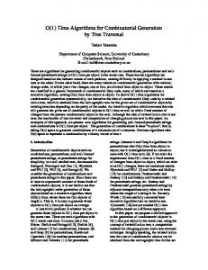
devices with valid exponential models are diodes, PNP transistors and MOS transistors operating in weak inversion [Wie93]. Recently, an emulation of a bipolar transistor has been proposed [DBS04], where a subnetwork structure of three CMOS transistors and one diode shows the necessary exponential behavior. In our circuit diagrams, we will use the symbol of a bipolar NPN transistor, shown in Figure 3.1, to represent an abstract �translinear device�, and we will simply use the term �transistor� for such an abstract device. It follows from the above that several di�erent silicon implementations of a �transistor� are possible.
collector base emitter Figure 3.1.: The symbol for a bipolar NPN transistor, our placeholder for a �translinear device�.
13
3. Translinear Network Theory
The ideal exponential model of a transistor is given by the equation
ICE = IS eVBE /UT , saying that its collector current
ICE
(3.1)
(the current from collector to emitter) is exponen-
VBE (the voltage between base and emitter). In IS and UT are device- and operation-dependent parameters called saturation current and thermal voltage, respectively. It is assumed that IS > 0 and UT > 0.
tially dependent on the base voltage this model,
We usually make the additional model assumption that the base current (the current from base to emitter) of a transistor is zero.
3.1.1. The Static Translinear Principle
translinear loops.
The key structures of translinear networks are so-called a loop
W
We call
of the network digraph a translinear loop if it satis�es the following three
properties:
• W •
consists exclusively of base-emitter branches of transistor.
All transistors involved share the same pair
• W
(IS , UT )
of parameters.
consists of as many forward branches as backward branches. Remember that
we regard the branches to point �from base to emitter�.
Figure 3.2 shows two examples for a translinear loop.
The interesting property of translinear loops is that due to the exponential transistor model, we can deduce a multiplicative relation of collector currents from
Kirchhoff
's
Voltage Law (KVL): Denote the base voltages of the transistors in W -forward orientaf f tion by V1 , . . . , Vr , the base voltages of the transistors in W -backward orientation by b b V1 , . . . , Vr . Then KVL for W reads
V1f + · · · + Vrf = V1b + · · · + Vrb .
I1f
I1b
I2f
I2b
I3f
I1f
I3b
I1b
I2f
Figure 3.2.: Examples for translinear loops.
14
I2b
3. Translinear Network Theory
Iout
Iin1 Q1
Q2
v1
v3
v2
Q3
Q4
Iin2
Figure 3.3.: A geometric mean circuit
Taking advantage of the common parameters, we deduce f
f
b
b
eV1 /UT · . . . · eVr /UT = eV1 /UT · . . . · eVr /UT and multiplication by
�
ISr �
V1f /UT
IS e
yields
�
Vrf /UT
· . . . · IS e
�
�
V1b /UT
= IS e
�
�
Vrb /UT
· . . . · IS e
�
.
Considering the model equation eqn. (3.1), this means exactly
I1f · . . . · Irf = I1b · . . . · Irb , where
I1f , . . . , Irf
base-emitter
Remark
(3.2)
I1b , . . . , Irb denote the collector currents of the branches are W -forward or W -backward, respectively. and
3.1. Note that
Is
and
UT
transistors whose
don't occur any more in eqn. (3.2). This means that
the relation between the collector currents holds independently of these parameters, provided they are indeed common. One nice e�ect of this is that translinear networks are essentially temperature-insensitive.
Example 3.2.
The loop indicated by thick lines in Figure 3.3 is a translinear one, being
made up of the base-emitter branches of transistors and
IS
Q1 , . . . , Q4 .
(We assume that
UT
1
coincide for the four transistors.) Application of the translinear principle yields
I1 · I3 = I2 · I4 . 1 Here we simply denote the collector current of a transistor in the following examples, too.
15
(3.3)
Qj
by
Ij .
We will stick to this convention
3. Translinear Network Theory
u1
Q1
y+
v1 Q2
u2
y-
Q3
v4
v2 Q4 v5
v3 Q5
Q6
Q7
v6
Figure 3.4.: A translinear frequency doubling network.
Genin
and
Konn
(Since its �rst publication by
in 1979 [GK79], this network has become a very promi-
nent example application of the translinear principle.)
Now remember our assumption that base currents are zero. Taking this into account, Kirchho� 's Current Law (KCL) for
v3 : I4 = I2 = Iout . Iin1 , Iin2 and Iout :
and for by
so
Iout =
√
v1
means that
I3 = Iin1 .
Similarly for
v2 : I1 = Iin2 ,
Thus we can substitute the collector currents in eqn. (3.3)
Iin2 · Iin1 = Iout · Iout ,
Iin1 · Iin2 (since Iout , being a collector current, must be positive).
That means,
the network �computes� the geometric mean of the two inputs.
Example 3.3.
As an example for a network with several translinear loops, consider the
network of Figure 3.4. Transistors
Q1 , Q2 , Q6 , Q5
form a translinear loop. The according equation is
I1 · I5 = I2 · I6 . Another translinear loop consists of transistors
Q3 , Q4 , Q7 , Q6 .
I3 · I6 = I4 · I7 .
(3.4) This gives (3.5)
By Kirchho� 's Current Law and our neglection of base currents, we can rewrite eqn. (3.4) and eqn. (3.5) as
u1 · u1 = y + · (y + + y − ), y − · (y + + y − ) = u2 · u2 .
16
3. Translinear Network Theory
A little computation reveals that
u2 − u 2 y+ − y− = p 2 2 1 2 . u 1 + u2 If we apply sinusoidal inputs with a
90◦
phase shift, like
u1 = |a sin t| , u2 = |a cos t| , with a �xed
a∈
R, then the di�erential output becomes y + − y − = a cos 2t,
that is, the network shows a frequency doubling behaviour for these inputs.
So every translinear loop leads to an equation of the form of eqn. (3.2). Summarizing the translinear principle in words:
In a loop of base-emitter branches of transistors with the same thermal voltage and the same saturation current, with an equal number of forward and backward branches, the product of collector currents of the transistors whose base-emitter branches are forward in the loop is equal to the product of collector currents of the transistors whose base-emitter branches are backward
2
in the loop.
3.1.2. Motivation for a Catalog of Topologies The following properties of static translinear (STL) networks can be observed from the examples of the preceding subsection:
•
STL networks can be described in terms of currents by systems of polynomial equations.
•
In such a system, no continuous parameters occur. This is due to the fact that and
•
IS
UT
vanish from the equations as soon as the STL principle is applied.
The topology of translinear networks satis�es strong constraints.
One of these
constraints is the condition that the number of forward and backward branches in a translinear loop be the same. Another constraint concerns the connection of collectors; it will be considered in Subsection 3.3.2.
2 This is the author's version of many similar formulations of the translinear principle as found in the literature [Gil68, pp. 364�365], [See88, p. 9], [Gil96, p. 107], [Min97, p. 6].
17
3. Translinear Network Theory
The second property means that the behavior of a STL network is already �xed by the network topology. In particular, there is only a �nite number of di�erent STL networks when the number of transistors is bounded! Together with the third property, which says that the number is not only �nite but also �not too large�, this observation has inspired the idea of a complete catalog of �small� STL networks.
If along with each network appropriate equations are stored, such a
catalog can serve as a design tool in an obvious way: When the designer is in search for a circuit with a given desired behavior, she or he can simply run through the catalog to �nd a network whose equations match that behavior. Chapter 5 of this thesis is about the details of the usage of such a catalog.
3.1.3. The Dynamic Translinear Principle For so-called dynamic translinear circuits, another circuit element comes into play: The capacitance. The symbol for a capacitance looks like this:
An ideal capacitance has the model equation
Icap = C V˙ cap , where of course
Icap
denotes the current through and
and the dot is used to denote time derivative.
capacity.
(3.6)
Vcap
the voltage across the element,
The device parameter
C > 0
is the
Consider a loop containing one capacitance and one or more base-emitter branches of transistors, as in Figure 3.5. This time, the branch orientations do not matter.
... C
...
Figure 3.5.: A dynamic translinear loop.
18
3. Translinear Network Theory
u1
u2
v1
Q1
Q2 y
Q3
v2
Q4
Q5
KVL for such a
Q6 C
v4
Figure 3.6.:
v3
A translinear integrating network. [See90]
dynamic translinear (DTL) loop is Vcap =
l X
±Vj ,
(3.7)
j=1 where the signs depend on the branch orientations. From eqn. (3.1) we deduce that
I˙j V˙ j = UT Ij for
j = 1, . . . , l,
so eqn. (3.6) and the di�erentiation of eqn. (3.7) yield
l X 1 I˙j Icap = UT ± . C Ij j=1
(3.8)
In short, the dynamic translinear principle says that for every DTL loop, eqn. (3.8) holds.
Example 3.4.
Figure 3.6 shows a translinear integrating network. The (static) translin-
ear loop equations for this network are
I1 · I4 = I2 · I5 , I3 = I4 , I6 = I5 .
19
(3.9) (3.10) (3.11)
3. Translinear Network Theory
There is a dynamic translinear loop consisting of the capacitance and, say, could as well consider the loop consisting of the capacitance and
Q2 , Q1
of the capacitance,
and
Q4 .)
Q6 .
(One
Q5 or the loop consisting
The according equation is
1 I˙6 Icap = UT . C I6
(3.12)
The node equations according to KCL are
and
I1 , . . . , I5
and
Icap
I3 = u1 I5 = I1 + u2 I4 + Icap = I2
for for for
v1 , v2 , v3 .
(3.13) (3.14) (3.15)
can be eliminated from eqns. (3.9) to (3.15), yielding
(u2 − I6 ) · u1 = (u1 + CUT
I˙6 ) · I6 , I6
which can be simpli�ed to
u2 · u1 = CUT I˙6 . If we assume the input
u2
to be a constant scaling factor, we see that the input
is proportional to the time derivative of the output
y = I6 .
u1
So indeed, the network
e�ectively performs integration. Although dynamic translinear networks have important applications, this thesis is mainly about STL networks, and capacitances won't occur very often. In particular, the implementation of a topological catalog as a synthesis tool, which has been produced in the framework of this thesis, is restricted to STL networks.
3.2. Translinear Decomposition of Polynomials We use the term �translinear decomposition� to denominate the process (or the result) of �nding a way of writing a polynomial
f ∈
Q[x1, . . . , xn] as an algebraic expression
which can be interpreted as one or more translinear loop equations. variables
x1 , . . . , x n
We think of the
as the inputs and outputs of a network to be designed, and of
f
as an implicit description of the network's desired behavior. Translinear decomposition is an important step of the design trajectory for translinear networks as described by Mulder et. al. [MSvdWvR99]. If one is only interested in networks with only one translinear loop, translinear decomposition amounts to �nding a way of writing
f
in the form
f = L1 · . . . · Lr − M 1 · . . . · M r ,
20
3. Translinear Network Theory
where
Li
and
Mi
are linear combinations of
x1 , . . . , x n .
An algorithm for translinear
decomposition in the 1-loop case is included in the work of Mulder et. al. [MSvdWvR99, pp. 91�107]. The author has developed an alternative algorithm [Ils02] and has compared both algorithms using implementations in
Mathematica.
In the general case of several translinear loops, translinear decomposition is much more complicated: Given
f,
we have to look for �translinear polynomials�
f1 =L11 · . . . · L1r1 −M11 · . . . · M1r1 , . . .
fs =Ls1 · . . . · Lsrs −Ms1 · . . . · Msrs (corresponding to
s
translinear loops) in the enlarged polynomial ring
Q[x1, . . . , xn, xn+1, . . . , xn+s−1] such that
f1 = · · · = fs = 0
x1 , . . . , xn+s−1 . Here ables x1 , . . . , xn+s−1 . The condition � f1 choosing
f1 , . . . , fs
the terms
implies
Lij
= · · · = fs = 0
and
f = 0 for Mij denote
any given set of real values for linear combinations of the vari-
f = 0� can be ensured algebraically by f lies inside the ideal hf1 , . . . , fs i, that is, in such [x1 , . . . , xn+s−1 ] with implies
in such a way that
a way that there exist
h1 , . . . , hs ∈
Q
f = h1 f1 + · · · + hs fs . Note that since
f
contains only
(3.16)
x1 , . . . , xn , the remaining variables xn+1 , . . . , xn+s−1 must
cancel on the right hand side of eqn. (3.16). No good algorithms are known for translinear decomposition in the general case (also called
parametric decomposition ),
and it doesn't seem probable that a satisfactory al-
gorithmic solution can be found, since the problem is in some sense �the wrong way around� compared to classical problems of computer algebra. Also, there are so many degrees of freedom that one can expect a very large number of solutions among which it would be complicated to recognize �good� ones. Another problem that arises when employing the �translinear decomposition� design trajectory is that it is not clear, once a suitable decomposition is found, how to make the collector currents in fact equal the linear combinations
Ljk
and
Mjk .
Still, it seems worthwhile to research about the algebraic problem of translinear decomposition. However, due to the problems mentioned, the design approach of this thesis avoids translinear decomposition.
21
3. Translinear Network Theory
3.3. The Topology of Translinear Networks In this section, we give a precise formulation of what a �translinear network� is in terms of graph theory. It will be the basic mathematical model of a translinear circuit's topology and consists essentially of a strict formulation of the constraints which the topology of translinear networks has to obey.
Although these constraints have all been known
before (their identi�cation is due to E. Seevinck [See88]), their translation into strict mathematics is new. The precise mathematical formulation is necessary for the speci�cation of the combinatorial task of compiling complete lists of topologies, considered in Chapter 4. It has been developed in collaboration with E. J. Roebbers and has been published earlier [Ils04, IR04]. The successful application (see Chapter 6) of the techniques of this thesis prove that the topological model �ts very well with the industrial needs.
3.3.1. Translinear Digraphs Translinear digraphs are the mathematical objects that are used to represent the core structure of a translinear network, the structure consisting of the translinear loops.
De�nition 3.5.
A
translinear digraph
is a digraph
G
satisfying the following prop-
erties:
1. Every loop of 2.
G
G
has as many forward branches as backward branches.
is biconnected.
One should think of a translinear digraph
G
as the digraph formed by the base-emitter
branches of a translinear network, that is, the branches of
G are in 1-to-1-correspondence e, tail(e) corresponds to the
with the transistors of the network, and for each branch
base node and head(e) to the emitter node of the respective transistor. Figure 3.7 shows the translinear digraphs of the example networks from Section 3.1.
22
3. Translinear Network Theory
e1
e2
v3
v1
v2
v1 e3
e4
e5
e1 v2
v5
v4 e6
e2
e7
v3
e4
e5 e6
e3 v4
v6 (a) The translinear digraph of the
(b) The translinear digraph of the inte-
frequency
grating network (Figure 3.6).
doubling
network
(see
Figure 3.4).
Figure 3.7.: Two translinear digraphs. The nodes carry the same names as in the corresponding networks; branch
ej
in the digraphs corrsponds to transistor
Qj
in Figure 3.4 or Figure 3.6, respectively.
Condition 1 in De�nition 3.5 obviously re�ects the main requirement on translinear loops as presented in Section 3.1.
The reason for including Condition 2 into the de�nition
is that the loops of di�erent biconnected components of the base-emitter digraph are decoupled, so we can consider the corresponding sub-networks seperately. The concept of a translinear digraph as the core of a translinear network was introduced by E. Seevinck [See88], although he concentrated on undirected graphs.
3
(Seevinck's
de�nition di�ers from the one given here in some more respects.) It turns out that condition 1 of De�nition 3.5 has a nice reformulation, as expressed by the following theorem:
Theorem 3.6. Let G be a digraph. The following two statements are equivalent: 1. Every loop of G has as many forward arcs as backward arcs. 2. There exists a map r : V (G) →
Z such that
∀ e ∈ E(G) :
r(tail(e)) = r(head(e)) + 1.
3 This is the reason that the term "translinear graph" is found very often in the literature, whereas "translinear digraphs" have not found much attention hitherto.
23
3. Translinear Network Theory
Proof. First assume there exists a map r as in statement (v0 , e1 , v1 , . . . , el , vl ), vl = v0 of G. By assumption,
2. Consider any loop
W =
r(vj ) = r(vj−1 ) − µ(W, ej ) for all
j = 1, . . . , l.
Inductively it follows that
r(vl ) = r(v0 ) −
l X
µ(W, ej )
j=1 and, because
vl = v0 , l X
µ(W, ej ) = 0.
j=1
µ(W, ej ) = ±1 for all j = 1, . . . , l, the latter is a sum of as many means that W contains as many forward arcs as backward arcs.
Since just
1's as -1's, which
For the other direction of the proof, assume that every loop contains as many forward arcs as backward arcs. In terms of incidence indices, this means
X
µ(W, e) = 0
(3.17)
e∈E(W ) for every loop
W.
It follows that eqn. (3.17) also holds if
W
is any cycle.
r with the stated property in the following way: For each connected C of G, pick an arbitrary vertex vC ∈ V (C). Then, for each vertex v ∈ V (C), P from vC to v and de�ne X r(v) := − µ(P, e).
Construct a map component �x a walk
e∈E(P ) It is now necessary to show that this de�nition is independent of the chosen walk let
P
0
be another walk from
vC
v. X
to
0=
Then
← − P ? P0
P.
So,
is a cycle and
← − µ(P ? P 0 , e)
← − e∈E(P ?P 0 )
X
=
µ(P, e) −
X
µ(P 0 , e),
e∈E(P 0 )
e∈E(P ) in particular
−
X
µ(P, e) = −
r(v)
µ(P 0 , e),
e∈E(P 0 )
e∈E(P ) which shows that
X
is indeed well-de�ned.
Applying this construction to every connected component gets the desired property: Let
e0 ∈ E(C)
C
of
G,
the map
be any branch of some component
24
r indeed C . If W
3. Translinear Network Theory
is a walk from de�nition of
vC
to tail(e0 ),
W 0 := W ? e0
is a walk from
vC
to head(e0 ), and by the
r, X
r(head(e0 )) = −
µ(W 0 , e)
e∈E(W 0 )
=−
� X
=−
� X
� µ(W 0 , e) − µ(W 0 , e0 )
e∈E(W )
� µ(W, e) − 1
e∈E(W )
=r(tail(e0 )) − 1.
It is clear that if a map map
r0
r
as in the second statement of Theorem 3.6 exists, so does a
that ful�lls the same condition as well as the additional property
min r0 (v) = 0.
(3.18)
v∈V (G) (Simply de�ne
r0 (v) := r(v) − 0min r(v 0 ).) v ∈V (G)
The nodes can then be partitioned into
�levels� or �layers�, such that a branch always points from one layer to the next lower layer:
V = V0 ∪˙ V1 ∪˙ . . . ∪˙ VR , where
Vj = { v ∈ V | r0 (v) = j}
Example 3.7.
and
In Figure 3.7(a),
In Figure 3.7(b),
R := max r0 (v). v∈V
R = 2, V0 = {v6 }, V1 = {v3 , v4 , v5 }
R = 2, V0 = {v4 }, V1 = {v2 , v3 }
De�nition 3.8. We call layered digraph.
This is illustrated in Figure 3.8.
and
and
V2 = {v1 , v2 }.
V2 = {v1 }.
a digraph ful�lling one and thus both conditions of Theorem
3.6 a
We see that a translinear digraph is nothing but a biconnected layered digraph. For any connected layered digraph, the additional property of eqn. (3.18) makes
r0
unique.
De�nition 3.9.
Let
r0 (v)
the
the integer
G
be a connected layered digraph. For a node
rank of v , and also denote it by rank(v).
v ∈ V (G),
In other words, the rank of a node is the index of the layer it belongs to.
25
we call
3. Translinear Network Theory
V3
V2
V1
V0 Figure 3.8.: layers of a translinear digraph
What is crucial about the layers of the translinear digraph of a network is that the rank of a node corresponds nicely to a certain range of the electric potential the node will have in an actual circuit. This is because the voltage drop along a base-emitter branch is always much larger than the swing of potential at one particular node. Since the rank is a node invariant, it also helps a lot in the classi�cation of translinear digraphs, as will become apparent in Chapter 4.
3.3.2. Connection of Collectors The previous subsection dealt with the base-emitter connectivity of a translinear network, which can be encoded in a translinear digraph. The main piece of information that is furthermore needed to describe a complete network is where to connect the collectors to.
e be a branch of a translinear digraph G. The collector of the transistor corresponding to e can only be connected to a node v of G if rank(v) > rank(head(e)). The reason is that head(e) is the emitter node, and the collector needs a higher potential than the
Let
emitter. E. Seevinck considered this condition in the construction of his �T-matrices� [See88]. We denote the collector node of a transistor corresponding to a branch digraph by
C(e).
Example 3.10. v3
and
e of the translinear
For the integrating network (Figure 3.6), we have
C(e5 ) = v2
(using branch names as in Figure 3.7(b)).
26
C(e3 ) = v1 , C(e4 ) =
3. Translinear Network Theory
But a collector does not necessarily need to be connected to a node of the translinear digraph.
It can also serve as a (current-mode) output of the network, or it can be
connected directly to a voltage supply. We will express this by
vext
as an additional node outside of
Example 3.11.
G.
In Figure 3.6/Figure 3.7(b),
C(e) = vext ,
imagining
C(e1 ) = C(e2 ) = C(e6 ) = vext .
In summary: A translinear network topology is speci�ed by
•
a translinear digraph
•
C : E(G) → V (G) ∪˙ {vext }, e ∈ E(G), either C(e) = vext or
G
and a map
rank(C(e))
where
C
has the property that for each
> rank(head(e)).
(3.19)
We identify
e tail(e) head(e) and C(e)
a branch
We call the map
C
the
with
a transistor,
with
the transistor's base node,
with
the transistor's emitter node,
with
the transistor's collector node.
collector assignment of the network.
(The notion of a collector
assignment will be re�ned in Section 3.4. )
Example 3.12. pair
(G, C),
We can describe the frequency doubling network of Figure 3.4 by the
where
G
is the translinear digraph depicted in Figure 3.7(a) and
C
is the
collector assignment
C(e1 ) =v1 , C(e2 ) =vext , C(e3 ) =vext , C(e4 ) =v2 , C(e5 ) =v3 , C(e6 ) =v4 , C(e7 ) =v5 . Remark
3.13. Note that in the latter example,
C(ej ) = tail(ej ) for j = 1, 4, 5, 6, meaning
that the collector is connected to the same node as the base of the respective transistor. In such cases of diode-like transistor usage, the condition expressed by eqn. (3.19) is �automatically� satis�ed, since by the de�nition of the rank of a node, rank(tail(e))
= rank(head(e)) + 1.
27
3. Translinear Network Theory
The information given by a translinear digraph
G and a collector assignment C
is already
a fairly complete description of a translinear network. In particular, a netlist for simulation or symbolic analysis of the network can be set up, if just some necessary �interface� information is added, for instance the connection of independent current sources which represent inputs of the network. These interfacing issues will be considered in Section 3.4.
3.3.3. Insertion of Capacitances The considerations of the preceding subsection are valid for STL networks as well as for DTL networks. But while the topology of a STL network is su�ciently modeled by a translinear digraph and a collector assignment, we must make one addition for DTL networks: How are capacitances allowed to be connected in the network? The answer is quite simple: A capacitance can be inserted between any pair of nodes of the translinear digraph. In Figure 3.6, for example, the capacitance branch is between node
v3
and the ground node
v4 ,
which are both nodes of the underlying translinear
digraph (see Figure 3.7(b)).
(G, C, Ecap ) of a translinear digraph Ecap of the set of 2-element subsets of
Thus, a DTL network topology is given by a triple
G, G.
a collector assignment (See also [IR04].)
C
Ecap
on
G,
and a subset
then consists of those pairs of nodes where a capacitance is
connected inbetween.
3.4. The Interface of a Translinear Network This section addresses the question of what should be considered as the �interface� of a translinear network, i. e. of how inputs are applied to and outputs are supplied by the network. Since the introduction of the translinear principle by Barrie Gilbert [Gil75] it is clear that inputs and outputs of a translinear network are in current mode.
3.4.1. Outputs All collectors which are designated �external� by the collector assignment collectors of those transistors for which
C(e) = vext )
C
(i. e., the
can be used as outputs of the
network. But not only the current of a single collector, also sums or di�erences of them can be considered as outputs. To be general, we consider a single symbolic output
y
of
a network which is a sum of positive and negative collector currents:
y=
X C(e)=vext
28
σ(e)xe ,
(3.20)
3. Translinear Network Theory
xe denotes the σ(e) ∈ {−1, 0, 1}. where
Example 3.14. −1.
collector current of the transistor corresponding to branch
For the frequency doubling network (Figure 3.4),
For the integrating network (Figure 3.6),
To avoid the usage of
σ,
σ(e1 ) = σ(e2 ) = 0
e
and
σ(e2 ) = 1 and σ(e3 ) = σ(e6 ) = 1.
and
we will henceforth work with the following re�ned concept of a
collector assignment: From now on, a collector assignment will be a map
C : E(G) → V (G) ∪˙ {vout+ , vout- , vvoid } such that for every
e ∈ E(G):
C(e) ∈ {vout+ , vout- , vvoid }
or
rank(C(e))
> rank(head(e)).
Thus, the symbolic output of a network will be (compare to eqn. (3.20)):
y=
X
X
xe −
xe .
(3.21)
C(e)=vout-
C(e)=vout+
3.4.2. Inputs and Ground Node Selection In principle, an independent input current iv can be applied to any node ear digraph
G.
v of the translin-
The only restriction is that the sum of all input and output currents
C(e) ∈ {vout+ , vout- , vvoid }) must always be which cannot be satis�ed if independent currents are prescribed for all nodes of G.
(the latter are now all collector currents with zero,
(In this case, the modelling assumptions about the transistors are not valid anymore.) Therefore, one has to select one particular node
v0
of
G
that serves as a �valve� whose
�dependent input� current results from values of the �true� inputs and of the outputs. (One should regard this dependence in terms of KCL for the ground node.) For convenience, we will always choose this �valve� node as the �reference� or �ground� node of the circuit, thus there will be no distinction between �valve node� and �ground node�, and we simply assume that we have an independent current source connected to each node of
G except one,
which we call the ground node and denote by
v0 .
We call all
other nodes �input nodes�. In the examples we have seen so far, most of the nodes of the translinear digraph have no current source connected to them. This amounts to an indepentent input which happens to be a constant zero and is not to be confused with the role of the ground node!
Example 3.15.
For the frequency doubling network (Figure 3.4):
v 0 = v 6 ; iv 1 = u 1 ,
iv2 = u2 , iv3 = iv4 = iv5 = 0.
Example 3.16.
For the integrating network (Figure 3.6):
iv3 = 0.
29
v 0 = v 4 ; iv 1 = u 1 , iv 2 = u 2 ,
3. Translinear Network Theory
A triple
(G, C, v0 )
of a translinear digraph
sense) and a ground node
v0
G,
a collecor assignment
C
(in the re�ned
is a network description which is complete in the sense
that the network equations can entirely be set up. The resulting system of polynomial equations will be studied in Section 5.1. That system contains all node equations but the one of
v0 .
For this reason, the current into the collector of the transistor corresponding
to a branch if
e with C(e) = v0
C(e) = vvoid ,
does not occur in the network equations. The same is true
e does a�ect C(e) ∈ V (G)\{v0 } or, if C(e) ∈ {vout+ , vout- },
while in all other cases, the collector current belonging to
the system: either in the node equation of in the output equation.
Hence, for the system of network equations, it does not matter whether
C(e) = v0 for a branch e. To avoid C(e) = v0 for any e. The simplest choose v0 ∈ V (G) \ img(C).
C(e) = vvoid
or
redundant entries in our catalog, we do not allow possibility to guarantee
C(e) 6= v0
for all
e
is to
We arrive at the following precise formal de�nition of a translinear network:
De�nition 3.17. of a translinear
(static) formal translinear network is a triple N = (G, C, v0 ) ˙ {vout+ , vout- , vvoid } and a node digraph G, a map C : E(G) → V (G) ∪ A
v0 ∈ V (G) \ img(C),
such that for every
C(e) ∈ {vout+ , vout- , vvoid }
e ∈ E(G): or
rank(C(e))
> rank(head(e)).
We call C the collector assignment of N and v0 the ground node of N . number of transistors of N is the number of branches of G.
The
3.5. Topologies for 4-terminal MOS transistors Next to bipolar transistors, subthreshold MOS transistors can be employed as �translinear device�. In the preceding sections, we frequently used a terminology that is adopted from the bipolar case. Speaking of MOS transistors, we should replace �base� by �gate�, �emitter� by �source� and �collector� by �drain�. But in addition to these three terminals, several authors have begun to use the �back gate� or �bulk� terminal of MOS transistors as an independent fourth terminal, instead of short-circuiting it �by law� with the source terminal [Ser05, MvdWSvR95, AB96, SGLBA99]. The topological concepts developed in the preceding sections are based on 3-terminal transistor devices. This section gives some ideas to adapt the concepts for 4-terminal MOS devices. However, a coherent description as for the 3-terminal case is not achieved. Our proposals are based on the �general translinear principle for subthreshold MOS transistors� by Serrano-Gotarredona, Linares-Barranco and Andreou [SGLBA99].
4
restrict to subthreshold MOS transistors employed in forward region. refer to the literature mentioned above.
4 We did the same for bipolar transistors by using eqn. (3.1) as model equation.
30
We
For examples, we
3. Translinear Network Theory
MOS translinear loops consist either of gate-source branches or of bulk-source branches. Analogously to the translinear digraph, which is the �base-emitter� digraph of bipolar translinear networks, we can consider a gate-source digraph digraph
Gbulk
of a MOS translinear network.
Ggate
and
Gbulk
Ggate
and a bulk-source
share a common node set
V := V (Ggate ) = V (Gbulk ), and furthermore, there is bijection
h : E(Ggate ) → E(Gbulk ) identifying branches representing the same transistor, such that tail(e) for each
e ∈ E(Ggate ).
= tail(h(e))
(Since both tails are to be identi�ed with the source of the
transistor.) According to [SGLBA99], it is not necessary to impose any loop condition similar to the one for the bipolar case (�as many forward as backward branches�) to
Ggate
or
Gbulk .
The biconnectedness condition applies to the �superposition� digraph
(V, E(Ggate ) ∪˙ E(Gbulk ), ι). The examples in [SGLBA99] show that neither
Ggate
nor
Gbulk
can be assumed to be
biconnected by itself, in fact, they cannot even be assumed to be connected. For connecting the drain terminals, one should require that they are provided with a higher potential than the corresponding source terminal.
Ggate
or
Gbulk ,
However, lacking layers of
we cannot use a convenient formal condition, like eqn. (3.19) for the
bipolar case, to express this requirement. In the example circuits known to the author, all drain terminals are either used as outputs or are short-circuited with the gate terminal of the respective transistor.
31
4. Combinatorial Generation of Translinear Networks The preceding chapter provides a way to regard translinear networks as formal combinatorial objects. This chapter describes techniques to generate complete lists of these formal objects, in order to compile catalogs of translinear networks which are exhaustive in the sense that they contain all possible topologies. Synthetic lists of translinear graphs and translinear digraphs have been produced before [See88, Wie93]. However, the idea to list complete network descriptions is new. The �rst section of this chapter introduces a common method in combinatorics to list graphs or other combinatorial objects. Since the core structures of translinear networks are translinear digraphs, Section 4.3 describes how to specialise the method for this particular class of digraphs, prepared by Section 4.2 on the generation of general digraphs. Sections 4.4 and 4.5 then deal with the exhaustive generation of collector assignments and complete formal networks for a given translinear digraph.
4.1. Orderly Generation This section describes orderly generation, a method for exhaustive generation of combinatorial objects. It was developed mainly by R. Read [Rea78]. It will be applied to the generation of formal translinear networks in the following sections. Subsection 4.1.1 introduces the general class of problems which orderly generation applies to.
Subsection 4.1.2 then covers the basic ideas of orderly generation, and in
Subsection 4.1.3 the main type of applications of orderly generation is presented.
4.1.1. Cataloging Problems The term �catalog� is used here to refer to a complete but redundance-free list of combinatorial structures such as elementary ones like sequences, permutations or partitions, but also more complex ones like graphs in several variants (simple graphs, multigraphs, digraphs, trees, colored graphs, etc.), designs [Dem97, And90, AK92, Col96, BJL99] or + linear codes [BFK 98, in particular chapter 3].
1
1 Of course, the literature provides plenty of more examples of combinatorial structures which a catalog makes sense of. In fact, structure is brought into the vast range of examples by a well-developed the-
32
4. Combinatorial Generation of Translinear Networks
1
3 3
2
1
4 2
4
0 1 0 0 0 0 0 0 Figure 4.1.:
0 1 0 0
0 1 0 0
0 0 0 0 0 0 1 1
0 0 0 0
0 0 1 0
Two labeled digraphs and their adjacency matrices.
Catalogs of these structures are useful in many respects: In pure mathematics, they can serve as a source of examples, especially for testing new conjectures. Also, classi�cation problems in many mathematical disciplines often boil down to discrete cataloging problems.
In practical applications, catalogs allow to get hands on error-correcting linear
codes, designs of agricultural experiments, isomers of a molecule, or, being the motivation of the present work, possible topologies of electrical networks. Main references for cataloging techniques, which can also be paraphrased as
generation
of structures,
are [Lau93, Lau99, GLM97, Rea78]. Related but not to be confused with
generation is
(counting) of structures, treated by [Red27, PR87, KT83,
enumeration
GJ83, dB64]. Both generation and enumeration are dealt with in [Ker99] or [KS99]. Except for the most simple structures, it is a nontrivial task to produce a catalog. The di�culties will become apparent after the following general formulation of a cataloging problem. Assume that for each
b∈
N, we have a �nite set Lb whose elements are easily digitally
represented and also easily listed in the sense that we can produce a list of all elements of in a time that is proportional to their number |Lb |. Furthermore, assume Lb ∩ Lb0 S∞ 0 for b 6= b ∈ and denote L := b=0 Lb . We call the elements of Lb the b.
Lb
N
structures of size
In the case of digraphs, for example, we take a �xed set of nodes of digraphs with node set
V
and exactly
b branches.
V
and let
Lb
be the set
Adjacency matrices are a convenient
digital representation of digraphs, and we can think of sum of entries is
=∅
labeled
Lb
as those matrices whose total
b.
Figure 4.1 shows two digraphs and their adjacency matrices. Since the matrices di�er, we have two di�erent elements of
Lb .
Unfortunately, the labeled structures are not yet what we are really interested in. Rather, we are interested in
unlabeled structures which are isomorphism classes of the labeled
structures. Since the two digraphs in Figure 4.1 are clearly isomorphic, we do not want ory of so-called
species
representing the types of combinatorial structures. [Ehr65, Joy81, BLL98],
see also [Ker99, pp. 1�20].
33
4. Combinatorial Generation of Translinear Networks
to have both of them in a list of �all digraphs with 4 nodes and 3 branches�, rather we want to have only one representative looking like this:
The example makes quite clear where the terminology �labeled� and �unlabeled� comes from.
Lb , where A ∼ B is to be interpreted 2 Thus, an as � A and B di�er only by their labelings� or � A and B are isomorphic�. unlabeled structure of size b is an element of Lb / ∼.
In general, we have an equivalence relation
∼
on
n nodes and b branches, the equivalence relation in terms of adjacency matrices is the one induced by the action of Sn consisting of simultaneous row and column permutations: Two n × n matrices A, B ∈ Lb are �isomorphic� if and only if there is a permutation σ which, when applied simultaneously to rows and columns, transforms A into B : In the case of digraphs with
A∼B
⇐⇒
(In Figure 4.1 above,
∃ σ ∈ Sn :
σ = (1 3)(2 4)
For all
i, j = 1, . . . , n : Bij = Aσ(i)σ(j) .
transforms the two matrices into each other.
σ
also
permutes the node labels of the two digraphs in the appropriate way.) The example of digraphs is presented here because digraphs are of course the structures we are speci�cally interested in for our purposes; further examples of labeled and unlabeled structures are nicely presented in the �rst chapters of [Ker99]. Quite an interesting example is the one of linear codes, where equivalence is isometry of codes, i.e. equivalent codes are guaranteed to show the same error-correcting behavior. In general, the best way to represent an unlabeled structure digitally is to represent it by one of the labeled structures it is made up of.
That means that we can de�ne a
U ⊂ L which has the property that for every A ∈ L there is a unique B ∈ U such that A ∼ B . In other words, U should contain exactly one element from each isomorphism class. Such a set U is called a complete system of representatives or a transversal of L/ ∼.
catalog as a subset
It is worth to point out that in principle, there is of course no problem to list unlabeled structures
completely :
One can just list the labeled structures. Every unlabeled structure
will be represented in the list at least once. The problem is that because in most cases it will be represented by quite a lot of labeled structures, the list gets very redundant
2 In more precise notation, one would use
∼b
instead of
however, cause any ambiguity. In fact, we can de�ne
A∼B
should imply that
A
and
B
∼
are of the same size.
34
∼.
Omitting the reference to
globally on
L=
S∞
b=1 Lb
b
does not,
by specifying that
4. Combinatorial Generation of Translinear Networks
and much too long, so that even when one just wants a complete list and redundance doesn't disturb by itself, the reduction of complexity obtained by eliminating isomorphs can be a great improvement of e�ciency. The naive approach for generating a transversal of
Lb / ∼
is expresssed by the following
pseudocode:
Algorithm 1 generateTransversal 1: 2: 3: 4: 5: 6: 7:
Ub := ∅
for all x ∈ Lb do if there is no u ∈ Ub
with
x ∼ u then
Ub := Ub ∪ {x}
end if end for return Ub
This algorithm is very slow because the isomorphism test very expensive, is performed very often.
u ∼ x,
which is in most cases
In the following subsection it will be shown
how this can be avoided.
4.1.2. Canonicity and Augmentation The basic idea to avoid the isomorphism test of Algorithm 1 is very intuitive: If we �nd some de�nition of �canonicity�, a property that exactly one element of each
∼-class
possesses, we can simply test all labeled structures for this property and thus
generate the set of �canonical� elements of
Lb ,
which is then our transversal of
Lb / ∼
:
Algorithm 2 generateCanonicalTransversal 1:
Ub := ∅
3:
for all x ∈ Lb do if x is canonical then
4:
Ub := Ub ∪ {x}
2:
5: 6: 7:
end if end for return Ub
This is a considerable improvement compared to Algorithm 1, because the so-far built
Ub
doesn't need to be searched through in each cycle.
Note that it does not matter for Algorithm 2 if we replace amounts to the same as successive generation of each of
U
Ub 's is substantial for Algorithm u ∈ U , instead of only u ∈ Ub , for
into the
all elements
35
Ub .
Ub
by the complete
U,
this
In contrast to this, the splitting
1, since in line 3 we would have to check being an isomorph of
x.
4. Combinatorial Generation of Translinear Networks
An appropriate de�nition of canonicity is easily found: Usually, the set
L
of labeled
structures is endowed with some natural total order, which comes from a numerical or lexicographical interpretation of the �labelings� and their digital representations.
For
example, one can imagine a 0-1-matrix (representing a simple labeled graph or digraph), read row by row, as a binary encoded integer. Thus, graphs are ordered by the integer ordering.
< on L, we simply de�ne the canonical representative one with respect to xk , xσ(k+1) ≥ 0 = xk+1 , . . .
xσ(l) ≥ 0 = xl , which means that all
(xσ )Σ > xΣ
, obviously a contradiction. So
k < j.
µ = 1, . . . , l, yσ(1)
≥
xσ(1)
=
. . .
. . .
x1
=
y1 ,
. . .
yσ(k−1) ≥ xσ(k−1) = xk−1 = yk−1 , yσ(k) ≥ xσ(k) > xk = yk . hence
yσ > y,
and the proof is �nished.
39
Since
yµ ≥ xµ
for
4. Combinatorial Generation of Translinear Networks
Having de�ned canonicity and augmentation, we are now able to catalog the G -orbits l in M by successive application of Algorithm 3, starting from L0 = {0}. Note that we have the case aug(x)
∩ aug(y) = ∅
for
x 6= y
as mentioned in Remark 4.2.
4.2. Generation of Digraphs Assume that we wish to build a catalog of the digraphs with integer
n.
n nodes for a given positive
As �digital representation� of digraphs we use adjacency matrices, thus we
take
L= as the set of labeled objects.
N0n×n
As the �size� of a digraph, we consider its number of
branches, so
) n X Ajk = b A ∈ L
( Lb = for
b∈
N0.
j,k=1
(Remember that both parallel branches and self-loops are allowed in our
de�nition of a digraph, see page 7.) This perception of �size� will be quite convenient later on, because for a translinear digraph, it re�ects the number of transistors of the respective network. If we view an
n × n -matrix as a word of length n2 , consisting of the concatenation of the
matrix rows, the number of branches is just the cross sum. That means, we can apply the generation of words presented in Subsection 4.1.3, to generate adjacency matrices. The permutation group to consider on the words of length
n2
is the image of the group
monomorphism
ι : Sn ,→ Sn2 de�ned by
ι(σ)(nj + k) = σ(j)n + σ(k) for
σ ∈ Sn , j = 0, . . . , n − 1 and k = 1, . . . , n. It will be more convenient, however, to Sn on the set of matrices, instead of a subgroup of Sn2 acting on
regard the action of the set of words.
An algorithm for the generation of all digraphs with specialisation of Algorithm 3:
40
n
nodes is derived easily as a
4. Combinatorial Generation of Translinear Networks
Algorithm 4 generateDigraphs(integer n > 0) 1: 2: 3: 4: 5:
U0 := {0n } for b := 1 to ∞ do Ub := ∅ for all A ∈ Ub−1 do for all A0 ∈ augword (A) do
if
6: 7: 8: 9: 10: 11: 12:
isCanonicalDigraph
0 (A )
0
then
Ub := Ub ∪ {A }
end if end for end for Output: Ub end for
(Here,
0n
denotes the
n×n
zero matrix.)
We can explicitely write down the canonicity test needed in line 6 of Algorithm 4:
Algorithm 5 isCanocialDigraph(square matrix A) 1: 2: 3: 4: 5: 6: 7:
n := n(A) for all σ ∈ Sn do if Pσ−1 APσ >lex A then
return false end if end for return true
The
>lex
comparison in line 3 of Algorithm 5 is meant as lexicographical comparison of
n(A) of A.
the words formed by concatenation of the matrix rows, and number of rows (which is equal to the number of columns)
in line 1 means the
Algorithm 4 is the basis for sophisticated and very fast graph generation systems that are used in particular for listing chemical isomers [Rea78, Ker99, Hea72, Gru93, GLM97, PR87, Pól37]. Algorithms 4 and 5 give a method to generate digraphs with a given number of nodes. When we use a digraph to model an electrical network, the number of branches is closely linked with the number of network elements. Thus it is indeed an appropriate measure of �size� or �complexity� of the network.
The number of nodes, in contrast, is quite
irrelevant. Therefore it is quite inconvenient for us that Algorithm 4 needs a number of nodes to be prescribed.
We would prefer an algorithm which generates digraphs
independly of the number of nodes. In the following, such an algorithm is developed.
41
4. Combinatorial Generation of Translinear Networks
Up to now, we use an augmentation that adds exactly one branch to a digraph and leaves the node set �xed. To get away from the �xed number of nodes, we can allow the insertion of new nodes while adding a branch: We consider not only the insertion of a branch between two existing nodes, but also a new branch from an existing to a new node or vice versa, or even a new isolated branch between two new nodes. We restrict to digraphs without isolated nodes. (It would be trivial, however, to generate all digraphs from those without isolated nodes. For our purpose, however, disconnected digraphs are irrelevant.) As before it is very helpful to discuss the augmentation by means of its reversal, the deletion of branches. We distinguish 4 cases when we delete a branch: 1. Neither tail nor head of the branch becomes isolated. This is the �standard� case which Algorithm 3 restricts to. 2. The head node becomes isolated and vanishes. The tail node stays. 3. The tail node becomes isolated and vanishes. The head node stays. 4. Both head node and tail node become isolated and vanish. The dimension (number of rows/columns) of the corresponding adjacency matrix of shrinks by 1 in cases 2 and 3, and it shrinks by 2 in case 4. In case 1, of course, the dimension does not change. We now consider in detail, for the 4 cases, how the adjacency matrix of the augmented digraphs can look like if the adjacency matrix of the branch-deleted digraph is
A.
1. The branch is inserted between two existing nodes. The adjacency matrix of the augmented digraph is one from aug
word (A).
2. The new branch points from an existing node to a new node. The adjacency matrix of the augmented digraph is one of
A→1
:=
A 0 ··· 0
1 0 A . . , . . . , A→n := . 0 0 ··· 0 0
0
. . .
. 0 1 0
3. The new branch points from a new node to an existing node. The adjacency matrix of the augmented digraph is one of
A←1 :=
0 A 1 0 ··· 0
. . .
A , . . . , A←n := 0 0 ··· 0 1 0
42
0 . . .
. 0 0
4. Combinatorial Generation of Translinear Networks
4. The new branch points from one new node to another. The adjacency matrix of the augmented digraph is
A↔
0 0 . . .
. . .
0 0
A := 0 ··· 0 0 ··· 0
. 0 0 0 1 0 0
(We do not take into account the matrix
A 0 ··· 0 0 ··· 0
. . .
. . .
, 0 0 0 0 1 0
because it is not canonical.)
Remark
4.4. If
A is canonical,
augmentations according to 2 or 4 always yield canonical
matrices. This is not the case for augmentations according to 3. We can use the following (non-terminating) algorithm to generate literally all digraphs without isolated nodes and without self-loops.
43
4. Combinatorial Generation of Translinear Networks
Algorithm 6 crossGenerateDigraph 1: 2: 3: 4: 5:
U0 := {(0)} for b := 1 to ∞ do Ub := ∅ for all A ∈ Ub−1 do for all A0 ∈ augword (A) do
if
6: 7: 8: 9: 10: 11: 12: 13: 14: 15: 16: 17: 18: 19: 20: 21:
isCanonicalDigraph
0 (A )
0
then
Ub := Ub ∪ {A }
end if end for for j = 1 to n(A) do Ub := Ub ∪ {A→j }
end for for j = 1 to n(A) do if isCanonicalDigraph(A←j ) then Ub := Ub ∪ {A←j }
end if end for
Ub := Ub ∪ {A↔ }
end for Output: Ub end for
4.3. Generation of Translinear Digraphs In this section, we explain how to adapt Algorithm 6 for the generation of translinear digraphs. First, in Subsection 4.3.1, we investigate the special structure of adjancency matrices of layered digraphs. Subsection 4.3.3 presents the augmentation and Subsection 4.3.2 the canonicity we use for layered digraphs. Subsection 4.3.4 brie�y tells how to restrict to translinear digraphs when applying the generation of layered digraphs. We can dispense with pseudocode in this section, the structure of the algorithms is clear from the pseudocode in the preceding sections.
4.3.1. Adjacency matrices of layer digraphs Consider the adjacency matrix of a layered digraph. Assume the digraph is connected, so the rank of each node is well-de�ned. Because we know that there can never be a
6= rank(v) + 1, we only need to store adjacency matrices �from one layer to the next�. If the maximal rank of any node of G is R, and (1) (R) (k) the number of nodes of rank k is nk , we need R matrices A , . . . , A , where A has branch from node
v
to node
w
if rank(w)
44
4. Combinatorial Generation of Translinear Networks
nk−1 × nk . This makes a total of n(n − 1)/2 entries we need to store
dimensions than the
PR
k=1 nk−1 nk entries, which is always less for the complete adjacency matrix. (We
3
continue to denote the total number of nodes by n, so here n = n0 + n1 + · · · + nR .) The (1) (R) matrices A , . . . , A can be regarded as blocks of the complete adjacency matrix, if we order the nodes according to their rank. Outside of these blocks are then only zeros: rank
0
rank
1
rank
2
rank
R−1
rank
rank
0
0
0
0
0
0
rank
1
A(1)
0
0
0
0
0
0
A(R)
0
rank
2
0
A
(2)
0 ..
rank
R−1
0
0
0
R
0
0
0
rank
R
.
..
.
..
.
So we represent a layered digraph by a tuple of matrices. Our set of labeled structures is
R positive integer, L = (A(1) , . . . , A(R) ) A(k) ∈ {0, 1}nk−1 ×nk for k = 1, . . . , R, . n0 , . . . , nR positive integers
The �size� is still the total number of branches, namely
b=
R n k−1 nk X X X
(k)
Aij .
k=1 i=1 j=1 Isomorphisms of layered digraphs consist of bijections of the node sets that preserve rank. These bijections decompose into permutations �inside� each rank. The equivalence relation to consider is the following.
De�nition 4.5.
A = (A(1) , . . . , A(R1 ) ), B = (B (1) , . . . , B (R2 ) ) ∈ L, we de�ne A ∼ B if and only if A and B have the same dimensions (n0 , . . . , nR ) (in particular R1 = R2 = R) and there exist permutations σ0 ∈ Sn0 , . . . , σR ∈ SnR such that for k = 1, . . . , R, i = 1, . . . , nk−1 , j = 1, . . . , nk : (k) (k) Bij = Aσk−1 (i)σk (j) . For
4.3.2. Canonicity
(A(1) , . . . , A(R) )
PR
k=1 nk−1 nk by reading the matrices one after the other, and each matrix word by word. Thus, a matrix tuple
We view a matrix tuple
3 The number
as word of length
n(n−1)/2 takes into account that a translinear digraph is acyclic, so with an appropriate
numbering of the nodes, the adjacency matrix has zeros in the lower triangular part as well as on the diagonal.
45
4. Combinatorial Generation of Translinear Networks
(A(1) , . . . , A(R) ) is canonical if and only an integer j , 1 ≤ j ≤ R, such that A(1)
if for all
(σ0 , . . . , σR ) ∈ Sn0 × · · · × SnR ,
there is
Pσ−1 A(1) Pσ0 , 1
= . . .
A(j)
Pσ−1 A(j) Pσj−2 , j−1
=
A(j+1) >lex Pσ−1 A(j+1) Pσj−1 , j where the inequation is to be omitted if
j = R.
The canonicity test can be performed by testing all permutation tuples
(σ0 , . . . , σR ) ∈
Sn0 × · · · × SnR . (For the implementation of the class �ranked� (see Appendix B), a re�ned and more e�cient version of the canonicity test is used that incorporates the successive computation of the automorphism group of the layered digraph.)
4.3.3. Augmentation As we distinguished 4 �augmentation cases� in the general digraph case, we distinguish 6 augmentation cases of layered digraphs. We classify them as sub-cases of the general digraph cases as follows:
1. No new node appears. The new branch is inserted between layer
AR
is replaced by an element of aug
2. The new branch points from existing node of rank
AR
R and layer R−1.
word (AR ). R
to a new node of rank
R − 1.
is replaced by
0 . . .
AR and a zero row is appended to
AR−1 .
, 0 1
(4.2)
(In contrast to the general digraph case,
there is only one possibility of this augmentation.
The � 1� does not appear at
another than the last position of the new column in eqn. (4.2), because otherwise decrementing the last non-zero entry would not yield
AR .)
3. The new branch points from a new node to an existing node. a) The new node appears in the top layer, the new branch points from layer to layer
R − 1. AR �
is replaced by one of
AR 1 0 ··· 0
�
46
� ,...,
AR 0 ··· 0 1
� .
R
4. Combinatorial Generation of Translinear Networks
b) The new node appears �above� the old top layer. A matrix
AR+1
to the matrix tuple, where
�
AR+1
is appended
is one of
�
1 0 ··· 0
,...,
�
0 ··· 0 1
�
.
4. Both head and tail of the inserted branch are new nodes. a) The new tail node has rank
R,
the new head node has rank
R − 1. AR
is
replaced by
and a zero row is appended to b) The new tail node has rank
0 AR 0 ··· 0
. . .
, 0 1
AR−1 .
R+1 (in particular, a new top layer is introduced), R. A zero row is appended to AR , and the matrix
the new head node has rank
AR+1 = [ 0 · · · 0 1 ] is appended to the matrix tuple. Note that the represented digraph is disconnected and that all further
canonical
augmentations of the matrix tuple
will represent a disconnected digraph.
4.3.4. Specialization for Translinear Digraphs Having derived techniques for the generation of layered digraph, we specialise them for the generation of translinear digraphs.
As translinear digraphs are nothing but
biconnected layered digraphs, we can simply generate all layered digraphs and �lter them for the biconnected ones. The algorithm of Tarjan [Jun99, p. 343] is available for e�ciently testing a (di)graph for biconnectedness. We can increase the e�ciency of the generation of translinear digraphs if we do not generate
all
layered digraphs but try to leave out those which are for sure never aug-
mented to a biconnected one (that is, not even after several augmentations). The �rst measure we take is to omit the augmentation 4b, because resulting digraphs would be disconnected. As second measure, we do not apply augmentation 3b whenever there are any leaf nodes (nodes with only one branch incident) in layers
0, . . . , R − 1.
Besides 4b,
augmentation 3b is the only augmentation introducing a new layer, and obviously, leaf nodes in the lower layers would stay �forever�, so that none of the digraphs obtained by repeated augmentation would be biconnencted. Orderly generation of translinear digraphs as described has been implemented in C++ and applied to list all translinear digraphs with 9 or less branches. As results, Figure 4.2
47
4. Combinatorial Generation of Translinear Networks
Figure 4.2.: The translinear digraphs with 6 or less branches.
4
shows the translinear digraphs with up to 6 branches , and the following table shows the numbers of the translinear digraphs with
b = 4, . . . , 9
branches.
number of branches:
4
5
6
7
8
9
number of translinear digraphs:
2
3
19
39
174
559
4.4. Generation of Collector Assignments In this section, we consider the generation of all collector assignments for a given translinear digraph
G.
De�nition 4.6.
C1 , C2 on G are called isomorphic if there ϕ : G → G such that C1 (ϕ(e)) = ϕ(C2 (e)) for every branch ϕ(vout + ) := vout+ , ϕ(vout- ) := vout- and ϕ(vvoid ) := vvoid .
Two collector assignments
is a digraph automorphism
e ∈ E(G),
where
De�nition 4.6 re�ects topological equivalence of collector assignments.
However, we
decide to use a broader notion of equivalent collector assignments, where the isomorphism classes comprise objects that might represent slightly di�erent topologies, but whose system of network equations will look the same.
De�nition 4.7. Two collector assignments C1 , C2 on G are morphic if there exist a digraph automorphism ϕ : G → G V (G)
such that
σ
permutes only the top layer of
G
called
generalized iso-
and a permutation
σ
on
and
ϕ(C2 (e)) = C1 (ϕ(e)) 4 Admittedly, the list of the 24 translinear digraphs with up to 6 branches can as well be compiled without computer. For space reasons, we do not list translinear digraphs with more branches, since such a listing could only consist of a computer-generated display of the adjacency matrices and not of the more pleasant diagrams.
48
4. Combinatorial Generation of Translinear Networks
whenever rank(C2 (e))
0.
R
R
The extended functionality (�simpli�cation using assumptions�) of the function
Simplify
Mathematica
[Wol99] performs this check satisfactorily.
In all example computations it was found that there is at most one ξ ∈ {1, . . . , dν } (ξ) min max max with xν (u) > 0 for all u ∈ ]u1 , u1 [× · · · × ]umin [. If there is none, a hardware s , us implementation of the network will not work, because the model assumption of positive collector currents is not satis�ed.
We can delete the pair
�candidates�.
58
(N, B)
from our set of
5. A Catalog of Topologies as a Synthesis Tool
But if there is indeed a positive solution for each collector current, we have determined the exact explicit dependence of the collector currents on
u1 , . . . , u s ,
and thus also the
exact explicit dependence of the output
y=
X
xe
C(e)=vout-
C(e)=vout+ on
X
xe −
u1 , . . . , u s .
5.4.2. Output Function Check After the positivity check of collector currents, we have an explicit description of the network behavior in the form
y = h(u1 , . . . , us ),
and we know that
g(u1 , . . . , us , h(u1 , . . . , us )) = 0. Still, it might be that the intended behavior was a di�erent branch of the solution of the polynomial equation g = 0. (For example, we may look for a network with y 2 thus specify g = y − u1 . Then the network search may yield a network with
√ = u1 and √ y = − u1 .
Of course, less pathological examples exist where the di�erence is more than the sign.) The comparison of
h
with the intended explicit behavior is our last check to �lter out
formal networks which are of no practical relevance. Both the positivity check of collector currents and the output function check have been implemented in
Mathematica
.
59
6. Example Application The following example comes from industrial applications at the company Analog Microelectronics GmbH (in the following: AMG). The problems, communicated by E. J. Roebbers from AMG, concern the question whether the nonlinear behavior of a certain sensor device can be compensated by a static translinear circuit.
This chapter is joint work
with E. J. Roebbers. A humidity sensor subsystem for air conditioning is in development at AMG. The sensor ◦ device to be used is optimized for an operating temperature of 23 C; at this temperature, its output is virtually proportional to the relative humidity.
For other temperatures,
it shows deviations from this linear behavior which are to be compensated.
For this
purpose, an �analog computation� circuit is desired to reconstruct the deviation. The circuit of course needs a second input where information about the actual temperature is provided independently of the sensor output. We denote the real relative humidity by humidity�) by
Hm .
H,
the output of the sensor (the �measured
The following information about the output deviation
Hm − H
at
some temperatures has been provided by AMG:
◦ -10 C
◦ 23 C
◦ 50 C
◦ 70 C
10%
-1%
20%
-1.5%
0%
1%
0%
1.5%
30%
-1.63%
0%
40%
-1.74%
0%
50%
-1.78%
0%
60%
-1.78%
0%
70%
-1.78%
0%
80%
-1.78%
90%
-1.78%
H
◦ 100 C
◦ 140 C
2%
3%
4%
3%
4.48%
6%
1.82%
3.55%
5.55%
7.43%
2.08%
4%
6.31%
8.35%
2.2%
4.2%
6.78%
8.78%
2.27%
4.35%
6.94%
9%
2.31%
4.43%
7%
9%
0%
2.31%
4.51%
7.12%
9%
0%
2.31%
4.51%
7.12%
9%
Since the desired circuit shall �compute� plot the points
(Hm , Hm − H)
Hm − H
from
for the above data:
60
Hm
(and the temperature
T ), we
6. Example Application
0.08 0.06 0.04 0.02 0.2
0.4
0.6
1
0.8
-0.02
The �rst task was to �nd an algebraic function
fspec
as speci�cation of a �translinear
synthesis� problem, so that these points satisfy (or are close to)
Hm − H = fspec (Hm , T ).
Mathematica-Functions FindMinimum ProjectiveRationalize (from the standard package NumberTheory`Rationalize`) have found the function fspec (Hm , T ) = λ(T )y(HM ), where
Some �educated guessing� and heavy usage of the and
λ(T ) = −0.0012167 (t − 10)(t − 1)(t + 3),
y(Hm ) = and
h = 0.3294.
2 + Hm hHm − Hm
The function
y
t=
T , 23◦ C
p
2 5h2 − 2hHm + Hm , 2h
(6.1)
is one of the two solutions of the implicit polynomial
equation
2 2 hHm + hHm y − Hm y − hy 2 = 0.
(6.2)
The following plot shows the surprisingly high quality of the approximation:
0.08 0.06 0.04 0.02 0.2
0.4
-0.02
61
0.6
0.8
1
6. Example Application
λ
consists of simple multiplications and can be implemented easily by translinear as
well as other analog circuitry, we don't go into further details of this part of the design problem. Instead we concentrate on the synthesis of a subcircuit implementing
y,
where the tools
developed in the framework of this thesis have been applied succesfully. The implicit description of the desired network behavior is given by (compare eqn. (6.2))
0 = g := u21 u2 + u1 u2 y − u21 y − u2 y 2 . The inputs are
u1 = Hm and u2 = h. (We h to the network.)
to supply the constant
use a stationary input current source for We wish to implement
g(u1 , u2 , y) = 0
u2
by a
circuit with at most 6 transistors. 15 of the 24 translinear digraphs with 6 or less branches consist of only one loop of length 4 and some parallel branches, see Appendix A. For these 15 digraphs, the toric ideal has exactly one generator of degree 2 and no generator of higher degree. Consequently, for all formal networks
3 = deg g ,
N = (G, C, v0 )
where
G
is one of these digraphs,
so the networks do not come into question for implementing
deg fN = 2