O(1) Time Algorithms for Combinatorial Generation by Tree Traversal Tadao Takaoka Department of Computer Science, University of Canterbury Christchurch, New Zealand E-mail:
[email protected] There are algorithms for generating combinatorial objects such as combinations, permutations and wellformed parenthesis strings in O(1) time per object in the worst case. Those known algorithms are designed based on the intrinsic nature of each problem, causing difficulty in applying a method in one area to the other. On the other hand, there are many results on combinatorial generation with minimal change order, in which just a few changes, one or two, are allowed from object to object. These results are classified in a general framework of combinatorial Gray code, many of which are based on a recursive algorithm, causing O(n) time from object to object. To derive O(1) time algorithms for combinatorial generation systematically, we formalize the idea of combinatorial Gray code by a twisted lexico tree, which is obtained from the lexicographic tree for the given set of combinatorial objects by twisting branches depending on the parity of the nodes. An iterative algorithm which traverses this tree will generate the given set of combinatorial objects in O(1) time as well as with a fixed number of changes from the present combinatorial object to the next. Although the idea of twisted lexico tree is not new, the mechanism of tree traversal and computation of changing places are new in this paper. As examples of this approach, we present new algorithms for generating well-formed parenthesis strings and combinations in O(1) time per object. The generation of combinations is done “in-place”, that is, taking O(n) space to generate combinations of n elements out of r elements. Previous algorithms take O(r) space to represent a combination by a binary vector of size r. 1. Introduction Generation of combinatorial objects such as combinations, permutations, and well-formed parenthesis strings, or parenthesis strings for simplicity, is a well studied area, documented in Reingold, Nievergelt and Deo [1], Nijenhuis and Wilf [2], Wilf [3], and Savage[4]. We consider the generation of combinations and parenthesis strings in this paper. Since there are at least an exponential number of those kinds of combinatorial objects, it is not hard to see that the lexicographic order generation of those objects based on a recursive algorithm takes O(f(n)) time, where there are f(n) objects of length n. That is, it is easy to generate those objects in O(1) time per object on average. A less trivial problem is whether we can generate those objects in O(1) time per object in the worst case. There are such algorithms with O(1) worst case time. To name just a few, Bitner, Ehrlich and Reingold [5], Ehrlich [6], and Lehmer [7] for combinations, Johnson [8] and Heap [9] for permutations, Korsh and Lipschutz [10] for multiset permutations, and Mikawa and Takaoka [11] for parenthesis
strings. Johnson’s and Heap’s algorithms for permutations take O(n) time from object to object, but it is straightforward to convert to ones with O(1) time as in [6]. If we relax the requirement from O(1) time to a fixed number of changes from object to object, which we refer to as O(1) changes, there are numerous results: Nijenhuis and Wilf [2] and Eades and McKay [12] for combinations, Proskurowski and Ruskey [13] and Ruskey and Proskurowski [14] for parenthesis strings, etc. Ruskey and Proskurowski generate parenthesis strings by adjacent transpositions only when n is even where the length of a string is 2n. Recently Walsh [15] successfully converted their recursive algorithm into an iterative one. Vjanowski [16] has yet another O(1) time algorithm based on a different approach. In this paper, we propose a unified approach to the generation of combinatorial objects in O(1) time per object in the worst case, using the concept of twisted lexico tree, a computation method for changing places, and a tree traversal technique. Roughly speaking, the twisted lexico tree for a set of combinatorial objects can be obtained from the lexicographic tree for the set
2
by twisting branches depending on the parity of each node. We give an even parity to the root. As we traverse the children of a node, we give an even and odd parity alternatingly to the child nodes. If a node gets even, the branches from the node remain intact. If it gets odd, the branches from the node are arranged in the reverse order. This concept of parity is applied to the entire tree globally, so that the constant change property can be easily shown for each set of combinatorial objects. The global parity is more transparent than the local parity in [11], which is defined locally in each subtree and useful only for parenthesis strings. The lexico tree and the concept of global parity were introduced in Zerling [17] and Lucas [18] respectively. The computation of changing places is done by identifying a changing place at any level of the tree, called the difference point, and the corresponding changing position down the tree, called the solution point. The concept of this paper can be viewed as a refinement of combinatorial Gray code introduced in Joichi, White and Williamson [19], Wilf [3] and Savage [4], which is in turn a generalization of the generation of binary reflected Gray code [20]. Based on this approach, we derive a new O(1) time algorithm for generating parenthesis strings in an order different from that in [11] and an in-place algorithm for generating combinations of n elements out of r elements in O(1) time per combination. Here “in-place” means it requires only O(n) space. Only O(1) average time is known for the in-place generation of combinations in Nijenhuis and Wilf [11] with the revolving door function which requires O(n) time in the worst case. Eades and McKay also considered an in-place algorithm, which generate combinations with O(1) changes but requires O(n) time. O(1) worst case time is known for combination generation in [5], [6], [7], and so forth, at the cost of O(r) space of a binary vector of size r to represent a set of n elements out of r elements. 2. Constant Change Generation Let Σ = {σ0, ... , σ r-1} be an alphabet for combinatorial objects. A combinatorial object is a string a1... an of length n such that each ai is taken from Σ and satisfies some property. A total order is defined on Σ with σ i < σ i+1. Let Σ n be the set of all possible strings on Σ of
length n. The lexicographic order < on Σ n is defined for a = a1...an and b = b1...bn by a < b ⇔ ∃ j (1 ≤ j ≤ n) a1 = b1, ... , aj-1 = bj-1, aj < bj. Let S ⊆ Σ n be a set of combinatorial objects. The order < on S is defined by projecting the lexicographic order on Σ n onto S. The lexicographic tree, or lexico tree for short, of S is defined in the following way. Each a ∈ S corresponds to a path from the root to a leaf. The root is at level 0. If a = a1...an, ai corresponds to a node at level i. We refer to ai as label for the node. We sometimes do not distinguish between node and label. If a and b share the same prefix of length k, they share the path of length k in the tree. The children of each node are ordered according to the labels of the children. A path from the root to a leaf corresponds to a leaf itself, so a corresponds to a leaf. The combinatorial objects at the leaves are thus ordered in lexicographic order on S. The twisted lexico tree of a set S of combinatorial objects is defined as follows together with the parity function. We proceed to twist a given lexico tree from the root to leaves. Let the parity of the root be even. Suppose we processed up to the i-th level. If the parity of a node v at level i is even, we do not twist the branches from v to its children. If the parity of v is odd, we arrange the children of v in reverse order. If we process all nodes at level i, we give parity to the nodes at level i+1 from first to last alternatingly starting from even. We denote the parity of node v by parity(v). When we process nodes at level i in the following algorithms, which are children of a node v such that parity(v)=p, we say the current parity of level i is p. Note that (labels of) nodes at level i are in increasing order if the parity of the parent is even, or equivalently if the current parity of level i is even. If the parity is odd, they are in decreasing order. We draw trees lying horizontally for notational convenience. We refer to the top child of a node as the first child and the bottom as the last child. If the labels on the paths from the root to two adjacent leaves in the twisted lexico tree for S are different at a fixed number of nodes, we can generate S with the fixed number of changes from object to object. We call the maximum number of changes the degree of S, denoted by deg(S). The above statement is restated as follows; if deg(S) is bounded by a
3
constant, we can generate S from object to object with the constant changes. In this case, we say S satisfies the constant change property (CCP). A general framework of a recursive algorithm for generating S with constant changes is given in the following. Since most variables take integer values, we omit variable
declarations. The current parity at level i is given by p[i], and the procedure “output” is only to see the result; for O(1) time this will be eliminated. We allow O(n) time for initialization. The parity 0 is for even and 1 for odd. Let Σ = {0, ... ,r-1}.
1. procedure generate(i); 2. var k; 3. begin 4. if i ≤ n then begin 5. if p[i] = 0 then 6. for k:=0 to r-1 do 7. if k is valid then begin 8. perform changes on a[i] and related positions; 9. generate(i+1) 10. end 11. else {p[i] = 1} 12. for k:=r-1 downto 0 do begin 13. if k is valid then begin 14 perform changes on a[i] and related positions; 15. generate(i+1) 16. end; 17. p[i]:=1-p[i] 18. end 19. else { i = n+1} output(a) 20. end; 21. begin {main program} 22. read(n); 23. initialize array a; 24. generate(1) 25. end. Algorithm 1. Recursive framework for generating combinatorial objects Note that this algorithm may generate S with constant changes, but it takes O(n) time from object to object in the worst case caused by the overhead time of recursive calls. In many applications, we perform changes on a[i] and a[j] for some j at lines 8 and 14. Then the objects, that is, array “a”, before and after the changes are different at i and j and the rests are the same. In this context, we say that the difference at i is solved at j. We refer to i and j as the difference point and the solution point. Generally the computation of the solution point is difficult and will depend on each application. 3. Recursion Removal
We devise in this section a general framework of an iterative algorithm which avoids the O(n) overhead time by recursive calls. Although this method is well known, we include this algorithm for other applications in this paper and show that the concept of parity can be maintained in the iterative algorithm. The array “up” is to keep track of positions of ancestors to which the algorithm comes back from leaves. Note that this algorithm takes O(1) time in the worst case if S satisfies the CCP and the changing mechanism is properly given. The variable “vi“ is for the next node to be processed at level i, which is maintained by some data structure in each application. A generic algorithm and illustration follow.
4
1. 2. 3. 4. 5. 6. 7. 8. 9. 10. 11. 12. 13. 14. 15.
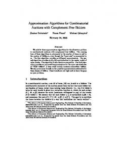
initialize array a to be the first object in S; initialize v1, ... , vn to nodes on the path to the first object (top path); for i:=0 to n do up[i]:=i; for i:=0 to n do p[i]:=0; repeat output(a); i:=up[n]; up[n]:=n; perform changes on a at vi and related positions; let vi go to the next node at level i based on the current parity; if vi is the last child of its parent then begin let vi further go to the next node at level i; up[i]:=up[i-1]; up[i-1]:=i-1; p[i]:=1-p[i] end until I=0. Algorithm 2. Iterative tree traversal
level i vi
up[n]=i
level n
w
object a next object a’
next vi
Figure 1. Going up and down When we come to the last child of a parent (w in the above figure), we have to update up[i] to up[i-1] so that when we visit the last leaf of the subtree rooted at w, we can come back directly from the leaf to w or its ancestor if w itself is a last child. We refer to the paths from vi to a and from next vi to a’ as the current path and the opposite path. A current path and opposite path consist of last children and first children respectively except for the left ends. If next vi in the above figure is a last child, we further set vi to the next node of next vi, say u, so we can avoid O(n) time to set up the environment for such u’s later. This is illustrated in the above figure by the path from “next vi” to “next object a’ ”. That is, when we traverse down the current path, we prepare for the opposite path so that we can jump over the opposite path from level i to the leaf.
5. Parenthesis Strings In this section, we consider the problem of generating all well-formed parenthesis strings of length 2n. We focus directly on the iterative algorithms based on Algorithm 2. We first define the characteristic sequence of a parenthesis string a = a1...an such that ai is the number of right parentheses between the i-th and (i+1)th left parentheses for i0 then swap(i+s[i]+1, i+s[i]+1+c[i]) else swap(i+s[i], i+s[i]+c[i]); s[i]:=s[i]+d[i]; if up[i-1]=i-1 or solved[i-1] then b:=s[i-1] else b:=s[i-1]-d[up[i-1]]; if (d[i]>0 and s[i]=i) or (d[i]


![[PDF] Ebook Combinatorial Optimization: Algorithms and Complexity ...](https://m.moam.info/img/260x300/pdf-ebook-combinatorial-optimization-algorithms-an_64785b96097c4796708cb897.jpg)