Algebraic Approaches for Centralized and Distributed Fault Identification in Discrete Event Systems∗ Yingquan Wu and Christoforos N. Hadjicostis†
Abstract In this paper we develop algebraic approaches for fault identification in discrete event systems that are described by Petri nets. We consider faults in both Petri net transitions and places, and assume that system events are not directly observable but that the system state is periodically observable. The particular methodology we explore incorporates redundancy into a given Petri net in a way that enables fault detection and identification to be performed efficiently, in a centralized or distributed manner, using algebraic decoding techniques. The guiding principle in adding redundancy is to keep the number of additional Petri net places small while retaining enough information to be able to systematically detect and identify faults when the system state becomes available. The end result is a redundant Petri net embedding that uses 2k additional places and enables the simultaneous identification of 2k − 1 transition faults and k place faults (that may occur at various instants during the operation of the Petri net). The proposed identification scheme has worst-case complexity of O(k(m + n)) (where m and n are respectively the number of transitions and places in the given Petri net) and can be extended to distributed settings in ways that require negligible additional hardware.
Keywords —Petri nets, discrete event systems, fault detection and identification, algebraic decoding, distributed fault diagnosis.
I
Introduction
A commonly used approach to fault diagnosis in dynamic systems is to introduce analytical redundancy (characterized in terms of a parity space) and diagnose faults based on parity relations [1, 2]. The methodology in [3] uses a similar idea to monitor faults in DES that can be modeled by Petri nets. In its most general form, this approach encodes the state (marking) of the original Petri net by embedding it into a redundant one in a way that preserves the state, evolution and properties of the original Petri net, while enabling an external mechanism to perform fault diagnosis. More specifically, faults in the Petri net transitions and/or places are identified via linear parity checks on the overall encoded state of the redundant Petri net embedding. Unlike analytical redundancy schemes for dynamic systems, the process of constructing a redundant Petri net embedding corresponds to adding ∗ This material is based upon work supported in part by the National Science Foundation under NSF Career Award No 0092696 and NSF ITR Award No 0085917, and in part by the Air Force Office of Scientific Research under Award No AFOSR DoD F49620-011-0365URI. Any opinions, findings, and conclusions or recommendations expressed in this publication are those of the authors and do not necessarily reflect the views of NSF or AFOSR. † The authors are with the Coordinated Science Laboratory and the Department of Electrical and Computer Engineering, University of Illinois at Urbana-Champaign. Address for correspondence: Christoforos N. Hadjicostis, 148 CSL, 1308 West Main Street, Urbana, IL 61801–2307, USA. E-mail:
[email protected].
1
redundancy in the system — in the form of additional places (sensors) and the connections (acknowledgments) associated with them. The benefit of this added redundancy is the ability to guarantee the quick detection of up to a certain (predetermined) number of faults in the system. In this paper we consider a setting similar to the one in [3] (fault identification in a DES that can be modeled by a Petri net) where activity (transition firing) is unobservable but the state (Petri net marking) is periodically observable. More specifically, at the end of a period we observe the final state (marking) of the redundant Petri net embedding and, based on this information, we need to detect and identify faults that may have occurred in this period. To achieve this, we construct redundant Petri net embeddings in which the identification of multiple and mixed (transition and/or place) faults, even when certain state information is missing, can be done systematically via algebraic coding/decoding techniques. Apart from fault detection and identification guarantees, our goal in choosing an appropriate redundant Petri net embedding is to keep the amount of redundancy (as indicated by the number of additional places/sensors) small. Since we are primarily interested in being able to handle complex, possibly distributed systems, we also develop a variation of our approach that is scalable and can be used in distributed settings. As we show in this paper, the use of a redundant Petri net embedding with 2k additional places (and the connections and tokens associated with them) allows the simultaneous identification of up to 2k − 1 transition faults and up to k place faults. The worst-case complexity of the fault identification procedure is O(k(m + n)) where m and n are the number of Petri net transitions and places respectively. The identification procedure is based on algebraic techniques, such as traditional decoding methods (e.g., Berlekamp-Massey decoding [4, 5]) and more recently developed methodologies for solving systems of composite power polynomial equations [6, 7]. Note that in order to achieve such efficiency in the identification process we need to add redundancy into the original Petri net. Since the occurrence of faults in large-scale discrete event systems (DES) can degrade their overall performance in unpredictable and possibly devastating ways, fault diagnosis and management in such systems has received considerable attention over the last two decades. In the remainder of this section we review this previous work, focusing primarily on approaches that are closely related to the scheme we present in this paper. In [8, 9], the DES is represented by a finite state machine (FSM) whose behavior is modeled as a regular language and faults are diagnosed using a diagnoser, i.e., an appropriately designed FSM that is capable of performing fault detection and identification by analyzing observable activity in the given FSM. Within this automata-based modeling formulation, these ideas are further extended in [10] where the authors study an integrated approach for diagnosis and control in DES by determining the sub-language of the legal language of a given DES that is supremely controllable, observable and diagnosable. Related approaches have also appeared for cases where failure specifications are given in linear temporal logic [11] or when there exist additional optimization objectives or other restrictions/requirements [12, 13, 14]. Apart from automata-based modeling formulations, previous work has also considered different DES models. For instance, the authors of [15] use a template language framework to represent a discrete event process, leading to on-line fault monitoring schemes for confirming correct system operation. In [16], the DES is modeled as a time Petri net and an analytical procedure for performing fault detection by back-firing transitions is developed. In [17], Petri net modeling is coupled with parameter trend and fault tree analysis to perform fault diagnosis. The monitoring of flexible manufacturing systems using colored timed Petri nets is investigated by [18]. Distributed and 2
asynchronous control/diagnosis in DES has been addressed more recently (see, for example, [19, 20, 21, 22, 23]). Also related to the work presented in this paper are diagnosis methodologies that identify faults in distributed settings using partially stochastic networks [24, 25]. The work in this paper is closely related to previous work that deals with observability properties of Petri net systems. For example, the authors of [26] (which provides an excellent background on this topic) present an approach to estimate the partially observable initial marking of a Petri net, given that the net structure is known and given that event occurrences are observable. In our setup, the initial and final states of the Petri net are known and our aim is to detect and identify faults that may have taken place during the evolution of the net, given that the event sequence is not observable but that the net structure is known. As evident from our analysis, our ability to detect and identify such faults depends critically on the amount of redundancy we add into the system. Finally, unlike [27, 28, 29, 30, 26], we do not discuss the issue of controlling the Petri net in a certain desirable way although it is possible that our approach here can be used in conjunction with such control strategies.
II
Preliminaries
A
Petri net notation
This section describes the notation and background needed for our Petri net development; more details can be found in [31, 32]. Petri nets can be used to model a variety of information and processing systems, including concurrent, asynchronous, distributed, nondeterministic, and/or stochastic systems, [32]. The functionality of a Petri net S is best described by a directed, bipartite graph with two types of nodes: places (denoted by {P 1 , P2 , ..., Pn } and drawn as circles) and transitions (denoted by {T1 , T2 , ..., Tm } and drawn as rectangles). Weighted directed arcs connect transitions to places and vice versa (but there are no connections from a place to a place or from a transition to a transition). The arc weights have to be nonnegative integers (we use b− ij to denote the weight of the arc from place Pi to transition Tj and b+ lj to denote the weight of the arc from transition Tj to place Pl ). Transitions denote system activity that causes the rearrangement, generation and consumption of tokens (which can be regarded as the resources that are available in the system). Places function as storage locations for tokens so that each place has a nonnegative integer number of tokens stored in it. At any given time instant t, the marking (state) of the Petri net is given by the number of tokens at its places. Transition T j is enabled (i.e., it is allowed to take place) only if each of its input places Pi has at least b− ij tokens. When transition Tj takes place (we say that + transition Tj fires), it removes b− ij tokens from each input place Pi , and deposits blj tokens to each output place 4
4
+ + Pl . If qs [t] denotes the state (marking) of the Petri net at time epoch t and B− = [b− ij ] (respectively, B = [bij ]) + denotes the n × m matrix with b− ij (respectively, bij ) at its ith row, jth column position, then the state evolution
of Petri net S is captured by qs [t + 1] = qs [t] + B+ x[t] − B− x[t] = qs [t] + Bx[t] ,
(1)
4
where B = B+ − B− and the input vector x[t] ∈ (Z+ )m indicates the transitions that take place (fire) at time epoch t (x[t] is usually assumed to be a unit vector with a single nonzero entry at its jth position indicating that transition Tj has fired). Note that transition Tj is enabled at time epoch t if and only if qs [t] ≥ B− (:, j) (where the inequality is taken element-wise and B− (:, j) denotes the jth column of B− ). 3
B
Fault model
Following the development in [3] we consider three different fault models, i.e., models that allow us to abstract away from the particulars of a system implementation and the hardware failure modes associated with it. Naturally, given a particular DES and its corresponding Petri net model, we need to ensure that our fault model effectively captures the faults that are expected in the system by mapping them into a manageable algebraic representation; we elaborate on this issue at the end of this section. (i) A transition fault models a fault in the mechanism that implements a certain Petri net transition. We say that transition Tj has a post-condition fault if no tokens are deposited at its output places (even though the tokens from its input places are consumed). Similarly, we say that transition T j has a pre-condition fault if the tokens that are supposed to be removed from the input places are not removed (even though tokens are deposited at the corresponding output places). + m + m Let e+ denote an indicator vector of post-condition faults and e− denote an indicator vector T ∈ (Z ) T ∈ (Z ) − of pre-condition faults. More specifically, the jth entry of e+ T (eT ) is a nonnegative integer indicating the number
of post-condition (pre-condition) faults that have affected transition T j . Then, the erroneous state qf [t] at time epoch t can be expressed as − − qf [t] = qs [t] − B+ e+ T + B eT ,
(2)
where qs [t] is the state that would have been reached under fault-free conditions [3]. (ii) A place fault models a fault that corrupts the number of tokens in a single place of the Petri net. A place fault at time epoch t results in an erroneous state qf [t] that can be expressed as qf [t] = qs [t] + eP ,
(3)
where qs [t] is the state that would have been reached under fault-free conditions and e P is an n-dimensional vector with a unique nonzero integer entry. More specifically, if eiP < 0 then the number of tokens in the ith place has decreased due to the fault, whereas if eiP > 0 then the number of tokens in the ith place has increased. Notice that when state information from a certain place is missing, one can assign zero (or an arbitrary value) as the number of tokens for this place and treat this situation as a place fault; therefore, place faults can also be used to model missing state information. (iii) The additive fault model is a generalization of the above fault models and is based on explicitly modeling each fault f by its additive effect ef on the fault-free state qs [t] that the Petri net would be in had the fault been absent, so that qf [t] = qs [t] + ef
(4)
for some appropriate ef ∈ Zn . Note that by combining (2) and (3), we can model the composite effect of transition and place faults on the erroneous state at time epoch t as − − qf [t] = qs [t] − B+ e+ T + B eT + e P .
(5)
It is also worth noting that the additive fault model can capture the effects of multiple faults. For example, if faults
4
− + − e+ 1,T , e1,T , e1,P occur at time epoch t1 and faults e2,T , e2,T , e2,P occur at time epoch t2 (t1 < t2 ), then the resulting
erroneous state at time epoch t2 will be − + − − qf [t2 ] = qs [t2 ] − B+ (e+ 1,T + e2,T ) + B (e1,T + e2,T ) + (e1,P + e2,P ) .
We will show that multiple such faults can be identified by performing checks periodically/non-concurrently, as long as we add enough redundancy to guarantee that information about the occurrence of faults is not lost. Our goal will be to add a small amount of redundancy so that we can achieve our goal using efficient detection/identification algorithms. Before closing this session, we would like to add a remark on fault modeling. Clearly, a pre-condition (postcondition) fault on a transition that has nT input (output) places can also be treated as a combination of nT place faults. Similarly, a fault whose additive effect is captured by a vector e f with nf nonzero entries can also be treated as a combination of nf place faults. In order for the fault identification mechanism to be able to resolve such conflicts, we aim at determining the minimum number of transition and/or place faults that explain the behavior observed in the Petri net. The underlying assumption in this formulation is that all transition and/or place faults are equally likely and independent (therefore, the most likely explanation is the one that involves the minimum number of faults).
C
Redundant Petri net embeddings
In [3] the identification of faults in a given Petri net S is facilitated by the construction of a redundant Petri net embedding H. More specifically, d places are added to the original Petri net S to form a composite Petri net H whose state (marking) qh [t] is η-dimensional (η = n + d, d > 0) and under fault-free conditions satisfies
qh [t] =
In C
qs [t]
(6)
for all time epochs t. Here, qs [t] is the state of the original Petri net S, In denotes the n × n identity matrix and C is a d × n integer matrix to be designed. In order to guarantee that (6) remains valid for all t, the state evolution of H is chosen to be of the form
B
qh [t + 1] = qh [t] +
+
x[t] −
+
CB − D | {z } +
B+ −
= qh [t] + (B − B )x[t] ,
B
−
x[t] CB− − D {z } | B−
(7)
where D is a d × m integer matrix, also to be designed. The d additional places together with the n initial places comprise the places of the redundant Petri net embedding H. In [3] it is shown that if matrices C and D have integer nonnegative entries and satisfy CB+ − D ≥ 0 and CB− − D ≥ 0 (element-wise), then a properly initialized redundant Petri net embedding H (i.e., one that satisfies Eq. (6) at t = 0) admits any firing sequence that is admissible in the original Petri net S. In other words, these choices for C and D ensure that the additional places do not inhibit any of the functionality in the original Petri net. Note that if the additional places do not
5
function as controllers but simply as sensors, then these constraints are not present (because the redundant Petri net embedding is then guaranteed to admit any firing sequence that is admissible in the original Petri net). By using a redundant Petri net embedding, we essentially introduce additional sensors in the system in a way that encodes the original state qs [t] into a codeword qh [t] that consists of the original state and the state of the added places. Although codeword-like constraints may already be present in the state of a given Petri net (in the form of place invariants for instance), in general we need to introduce additional places to enforce such constraints. 4
The validity of the codeword can be checked by using the parity check matrix P = [−C Id ] to verify that the syndrome s[t]
4
=
Pqf [t]
=
[−C Id ]qf [t]
(8)
(where qf [t] is the possibly faulty state at time epoch t) is zero. A nonzero syndrome at time epoch t indicates the presence of one or more faults. Faults can be identified based on the syndrome s[t] if matrices C and D are designed so that each combination of faults results in a unique syndrome. Notice that in order to verify (8) the fault identification mechanism needs to know the number of tokens in each place of the redundant Petri net embedding.
D
Problem formulation
We assume that the firing of transitions in the redundant Petri net is not directly observable while the Petri net marking is periodically observable. We aim to identify faults based on the observed marking at the end of a period. We use the term “non-concurrent” to capture the fact that diagnosis is performed over a period of several time epochs, in this case once every N time epochs. We assume that each transition may not suffer both pre-condition and post-condition faults within the epoch interval [1, N ] (actually, if a particular transition suffers both a precondition and a post-condition fault within [1, N ], their effects will be cancelled, making their non-concurrent detection impossible). + m + m Let e+ denote an indicator vector of post-condition faults and e− denote an indicator vector T ∈ (Z ) T ∈ (Z )
of pre-condition faults within the epoch interval [1, N ]. Assuming no place faults, the erroneous state q f [N ] at time epoch N is given by − − qf [N ] = qh [N ] − B + e+ T + B eT ,
(9)
where qh [N ] is the state that would have been reached under fault-free conditions. The fault syndrome at time epoch N is then 4
sT [N ] = Pqf [N ] = [−C Id ](qh [N ] − B + e+ + B − e− T) T − B+ B e+ + e− = [−C Id ] qh [N ] − T T CB+ − D CB− − D and is easily calculated to be sT [N ] = DeT , 6
(10)
4
− where eT = e+ T − eT . Clearly, the identification of transition faults based on the syndrome s T [N ] is completely
determined by matrix D. For example, if we choose all columns of D to be distinct (and not the negatives of each other), we can identify any single transition fault (as well as its type); as discussed later, more sophisticated designs of D allow us to efficiently identify multiple transition faults using algebraic techniques. Assuming no transition faults, place faults within the time epoch interval [1, N ] result in a corrupted state qf [N ] = qh [N ] + eP ,
(11)
where qh [N ] is the state that would have been reached under fault-free transitions and e P ∈ Zη denotes the (accumulated) place fault vector. The fault syndrome in this case is given by 4
sP [N ] = Pqf [N ] = PeP ,
(12)
i.e., the identification of place faults is exclusively determined by P. For example, if we choose C such that any two columns of P = [−C Id ] are linearly independent, then any single place fault is identifiable. Again, as discussed later, more sophisticated choices of C allow us to identify multiple place faults. Moreover, careful choices of both D and C enable the efficient identification of multiple and mixed (transition and/or place) faults.
III
Mathematical Background
In this paper we frequently make references to operations in GF(p), the Galois field of order p, where p is a prime number. In these fields, addition and multiplication can essentially be treated as addition and multiplication modulo p. For notational simplicity, we define 4
Λτ (x1 , x2 , . . . , xr ) = (−1)τ
X
xi1 xi2 . . . x iτ ,
τ ≤r,
(13)
1≤i1 r in the previous paragraph. Clearly, for i = 1, 2, . . . , r, we have 4
Λi = Fi (S1 , S2 , . . . , Si ) ¯ ¯ 1 ¯ S1 ¯ ¯ S1 ¯ S2 (−1)i ¯¯ . . .. = ¯ . i! ¯ . ¯ ¯ Si−1 Si−2 ¯ ¯ ¯ Si Si−1
0
...
0
2 .. .
... .. .
0 .. .
Si−3
...
S1
Si−2
...
S2
¯ ¯ ¯ ¯ ¯ 0 ¯ ¯ .. ¯ ¯ . ¯ ¯ i − 1 ¯¯ ¯ ¯ S1
0
and the Λi are independent of the number of original variables x1 , x2 , . . . (note that since Λi has a factor of
(18)
1 i! ,
the
Fi for i = 1, 2, . . . , r are well defined only if p > r). Now, we deduce this observation to a particular condition, as identified in the following proposition. Proposition 2 Let x1 , x2 , . . . , xr be r variables and s1 , s2 , . . . , sτ be τ known parameters in GF(p) with p > τ . Then, Fτ (s1 + S1 , s2 + S2 , . . . , sτ + Sτ ) is a linear combination of Λl , l = 1, 2, . . . , r. Moreover, min{r, τ }
Fτ (s1 + S1 , s2 + S2 , . . . , sτ + Sτ ) =
X
Fτ −i (s1 , s2 , . . . , sτ −i ) · Λi .
(19)
i=0
22 The proof can be found in [6, 7].
IV
Centralized Fault Identification
In this section we discuss centralized fault detection and identification, first for transition faults, then for place faults and eventually for combinations of transition and place faults. In each case, the diagnoser aims at identifying the combination of transition and/or place faults that has minimum cardinality and explains the observed behavior. 8
A
Identification of transition faults
In this section we discuss centralized identification of up to k transition faults within the epoch interval [1, N ]. The expression in Eq. (10) indicates that k or less transition faults are identifiable via a parity check if and only if the 4 Pm syndrome for transition faults sT [N ] = DeT is unique for any eT such that |eT | = i=1 |eiT | ≤ k (by assumption no cancellations take place in eT , i.e., no transition suffers both pre-condition and post-condition faults within the
− epoch interval [1, N ], which implies that |eT | = |e+ T | + |eT |). In the following analysis, we aim at designing matrix
D to achieve this objective. Consider the following choice for matrix D:
Dk+1
4 =
1
1
1
...
1
2
3
...
1 .. .
22 mod p .. .
32 mod p .. .
... .. .
1
2k mod p
3k mod p
...
where p is a prime number larger than m (the subscript
k+1
1
2 m mod p , .. . mk mod p m
(20)
is used to indicate the row dimension of D, which is
essentially the number of additional places). Note that matrix C does not directly 1 enter the development here and we consider it later when we discuss identification of place faults. We now demonstrate that the above choice for matrix D allows the identification of up to k transition faults by 4
establishing that the fault syndrome sT [N ] = [s0 s1 s2 . . . sk ]T = DeT is nonzero and unique for any eT that 4 Pm 4 − satisfies |eT | = i=1 |eiT | ≤ k. Note that s0 = |e+ T | − |eT | (for notational simplicity we let τ = s0 ). Without loss of generality, we assume that τ ≥ 0 and show that each combination of up to k faults causes a unique (nonzero)
syndrome sT [N ], implying that all combinations of up to k transition faults are identifiable. Suppose that a combination of τ + i post-condition faults and i pre-condition faults at transitions [x 1 , x2 , . . . , xτ +i , xτ +i+1 , . . . , xτ +2i ] (τ + 2i ≤ k) results in the same syndrome as a combination of τ + j post-condition faults and j pre-condition faults at transitions [y1 , y2 , . . . , yτ +j , yτ +j+1 , . . . , yτ +2j ] (τ + 2j ≤ k). Then, the following equation array holds: P Pτ +2j Pτ +j Pτ +2i τ +i (xl mod p) − l=τ +i+1 (xl mod p) = s1 = l=1 (yl mod p) − l=τ +j+1 (yl mod p), l=1 Pτ +i 2 Pτ +2i Pτ +j 2 Pτ +2j 2 2 l=1 (xl mod p) − l=τ +i+1 (xl mod p) = s2 = l=1 (yl mod p) − l=τ +j+1 (yl mod p), .. . Pτ +2j Pτ +j k P P τ +2i τ +i k k k l=τ +j+1 (yl mod p), l=1 (yl mod p) − l=τ +i+1 (xl mod p) = sk = l=1 (xl mod p) −
(21)
where τ + 2i ≤ k, τ + 2j ≤ k. We can weaken and rewrite (21) in the following form: P Pτ +2j Pτ +j Pτ +2i τ +i l=1 xl + l=τ +j+1 yl ≡ l=1 yl + l=τ +i+1 xl , Pτ +j 2 Pτ +2i Pτ +i 2 Pτ +2j 2 2 l=τ +i+1 xl , l=1 yl + l=τ +j+1 yl ≡ l=1 xl + .. . Pτ +j k Pτ +2i Pτ +i xk + Pτ +2j k k l=1 l l=τ +j+1 yl ≡ l=1 yl + l=τ +i+1 xl ,
(22)
1 Recall that if the additional places function as controllers, then one has to ensure that the redundant Petri net embedding H admits all firing sequences that are admissible in the original Petri net S by choosing matrix C to have nonnegative integer entries and satisfy CB+ − D ≥ 0 and CB− − D ≥ 0 (element-wise).
9
where the equality is now taken modulo p. For notational simplicity, in the sequel we use the notation “≡” to stand for equality modulo p. Since τ + i + j ≤ k and since no cancellations are allowed, we can use Proposition 1 to argue that i = j and that, ignoring order, {x1 , x2 , . . . , xτ +2i } = {y1 , y2 , . . . , yτ +2j }. This establishes the uniqueness of syndrome sT [N ] under this combination of transition faults. Therefore, the matrix D defined in (20) allows the identification of k or less transition faults. Next, we establish an efficient identification algorithm. Without loss of generality, we assume that τ + r postcondition faults and r pre-condition faults have taken place (τ + 2r ≤ k) and consider the following equation array:
P Pτ +2r τ +r l=1 (xl mod p) − l=τ +r+1 (xl mod p) Pτ +2r Pτ +r 2 (x2 mod p) (x mod p) − l=1
l=τ +r+1
l
l
= s1 , = s2 , .. .
(23)
Pτ +r (xτ +2r mod p) − Pτ +2r τ +2r mod p) = sτ +2r . l=1 l=τ +r+1 (xl l
We can weaken and rewrite (23) in the following form: P τ +r l=1 xl P τ +r 2 l=1 xl
≡ s1 + ≡ s2 + .. .
Pτ +2r
l=τ +r+1
Pτ +2r
l=τ +r+1
xl , x2l ,
(24)
Pτ +2r Pτ +r xτ +2r ≡ s τ +2r . τ +2r + l=1 l l=τ +r+1 xl We recall that Λl (x1 , x2 , . . . , xτ +r ) = 0 for l > τ + r. Using this observation in conjunction with Proposition 2, we conclude that for l > τ + r
0 = Λl (x1 , . . . , xτ +r ) ≡ Fl (s1 +
τX +2r
xj , . . . , s l +
j=τ +r+1
=
r X
τX +2r
xlj )
j=τ +r+1
Fl−j (s1 , . . . , sl−j ) · Λj (xτ +r+1 , . . . , xτ +2r ) .
j=0
By taking l = τ + r + 1, τ + r + 2, . . . , τ + 2r, we obtain the following linear equation array: P r j=1 Fτ +r+1−j (s1 , . . . , sτ +r+1−j ) · Λj (xτ +r+1 , . . . , xτ +2r ) ≡ −Fτ +r+1 (s1 , . . . , sτ +r+1 ), P r j=1 Fτ +r+2−j (s1 , . . . , sτ +r+2−j ) · Λj (xτ +r+1 , . . . , xτ +2r ) ≡ −Fτ +r+2 (s1 , . . . , sτ +r+2 ), .. . P r ≡ −Fτ +2r (s1 , . . . , sτ +2r ). j=1 Fτ +2r−j (s1 , . . . , sτ +2r−j ) · Λj (xτ +r+1 , . . . , xτ +2r )
(25)
As is readily seen, system (25) can be efficiently solved by the Berlekamp-Massey algorithm (cf. [4]) at the computational complexity of O(k 2 ). We are now ready to discuss the specifics of the identification procedure:
Transition Fault Identification Procedure 1. The first stage utilizes (16) (or (18)) to compute sequentially F1 (s1 ), F2 (s1 , s2 ), . . . , Fk (s1 , s2 , . . . , sk ); this stage requires O(k 2 ) operations. 10
2. For r = b(k−|τ |)/2c, apply the Berlekamp-Massey algorithm to solve for Λ l (xτ +r+1 , . . . , xτ +2r ), l = 1, 2, . . . , r; this can be accomplished with O(r 2 ) operations. 3. Substitute the obtained Λl (xτ +r+1 , . . . , xτ +2r ), l = 1, 2, . . . , r, into Eq. (17) and, using Proposition 1, obtain the solution of xτ +r+1 , . . . , xτ +2r by testing 1, 2, . . . , m, one by one; this is successful only if the solution exists and takes O(mr) steps. 4. With known xτ +r+1 , . . . , xτ +2r , we obtain Si (x1 , x2 , . . . , xτ +r ) = si −
Pτ +2r
l=τ +r+1
xil , i = 1, 2, . . . , τ + r, with
O(r(τ + r)) steps; we can then follow (16) to get Λ1 (x1 , . . . , xτ +r ), . . ., Λτ +r (x1 , . . . , xτ +r ) in O((τ + r)2 ) steps. 5. Substitute the values obtained in (iii) into (17) and follow Proposition 1 to get the solution of x 1 , . . . , xτ +r , again by testing 1, 2, . . . , m one by one (this is successful only if the solution exists). Clearly, the overall decoding/identification complexity of the procedure described above is O(k 2 m). Note that, for k = 1, the first row of matrix D in (20) is redundant; thus, we only need 4
D1 = (1, 2, . . . , m),
k = 1.
(26)
For k = 2, the first row is again redundant. This is justified by the fact that the equation array x ≡x +x 1 2 3 x2 ≡ x 2 + x 2 1 2 3 does not have a nonzero (non-trivial) solution2 in GF(p); thus, there is no confusion on the number of faults. Therefore, for k = 2, we can use the following matrix D: 4
D2 =
1
2
3
...
m
1
22 mod p
32 mod p
...
m2 mod p
,
k = 2.
(27)
Note that there is a variety of ways in which one can introduce additional places in order to capture pre-condition or post-condition transition faults. For example, a simple (but expensive) approach would be to do the following: (i) add one additional place for each transition; (ii) connect each additional place with its corresponding transition with one input and one output arc, both with unit weight; (iii) initialize each additional place with k tokens. Clearly, if the number of tokens in an additional place is k 0 6= k, then the corresponding transition has suffered a fault; in fact, if k 0 > k then the transition has suffered k 0 − k pre-condition faults, whereas if k 0 < k then the transition has suffered k − k 0 post-condition faults. Clearly, the task of the fault identification mechanism under this scenario is very simple, however, the amount of redundancy added in the system is prohibitively expensive, particularly for systems with a large number of transitions. Another significant disadvantage of this approach is that a single place fault in one of the additional places will lead to an erroneous diagnosis. The next section discusses how one can construct redundant embeddings that allow the systematic identification of place faults (assuming no transition faults); we then discuss more elaborate approaches which can be used to handle combinations of transition and place faults. 2 We
observe that x22 + x23 ≡ (x2 + x3 )2 yields 2x2 x3 ≡ 0 which implies that either x2 ≡ 0 or x3 ≡ 0.
11
B
Identification of place faults 4
We now focus on designing matrix P = [−C Id ] so as to identify up to k place faults with some d additional places (assuming no transition faults). This is equivalent to choosing the integer entries of the d × n matrix C so that the syndrome at time epoch N , which was shown in Section II.D to be equal to s[N ] = PeP , has a unique solution eP ∈ Zη with at most k nonzero entries. This is reminiscent of a decoding problem in which a message of length n is extended to a codeword of length n + d = η in a way that allows the correction of a maximum of k errors in the codeword. We will pursue this connection more explicitly for a special class of linear block codes, namely Reed-Solomon codes in GF(p) [4, 5]. For simplicity, for the remainder of this section all operations are defined in GF(p), unless stated otherwise. Let α be a primitive element in GF(p), i.e., an element such that {1, α1 , α2 , . . . , αp−2 } = {1, 2, 3, . . . , p − 1}. The parity check matrix of a Reed-Solomon code is defined in GF(p) as
Ht =
1
α1
α2
α3
...
1
α2
α4
α6
...
1 .. .
α3 .. .
α6 .. .
α9 .. .
... .. .
1
αt
α2t
α3t
...
αp−2
α2(p−2) α3(p−2) . .. . t(p−2) α
The set of codewords in the above code is formed by all (p − 1)-dimensional vectors c = [c 1 c2 . . . cp−1 ]T that satisfy Ht c = 0. This particular Reed-Solomon code has minimum Hamming distance 3 t + 1, i.e., the Hamming distance between any two codewords c and ˜ c satisfies dH (c, ˜ c) ≥ t + 1, which implies that the corruption of up to b 2t c entries in a codeword is correctable. Moreover, the solution of s = Ht e for a vector e with at most b 2t c nonzero entries in GF(p) can be achieved efficiently with computational complexity O(tp) using the Berlekamp-Massey algorithm. To transform our problem to the decoding of a Reed-Solomon code, we make (for now) the reasonable assumption that the number of erroneous tokens in a place is bounded. More specifically, we assume that e Pi , the erroneous number of tokens in place Pi , is within the interval [− p−1 2 ,
p−1 2 ],
where p is a large enough prime number. Under
this assumption, ePi can be interpreted to fall within [0, p−1] in GF(p) (by naturally mapping ePi to ePi (mod p)). This artificially imposed requirement enables us to transform our identification problem to the decoding of ReedSolomon codes. More specifically, what we need to do is to transform the problem in (12) (in which P is a systematic parity check matrix with integer entries) to the form s = Ht e discussed above. Note that one can always write ˜ It ] , Ht = Φ[−C 3 The Hamming distance d (x, y) between two vectors x = (x , x , ..., x ) and y = (y , y , ..., y ) with elements in GF(p) is the η η 1 2 1 2 H number of entries at which x and y differ [4, 5].
12
where matrix Φ denotes the last t columns of Ht (because Φ forms a nonsingular Vandermonde matrix [4, 5]). ˜ It ] = Φ−1 Ht (by interpreting the entries as integer entries in [0, p − 1], i.e., by inverting Clearly, if we set P = [−C the natural mapping mentioned above), then we can easily reduce (12) to a decoding problem. By taking both sides of (12) modulo p we obtain ˜ It ]eP sP [N ] = Pqf [N ] = [−C
⇒
sP [N ] ≡ Φ−1 Ht eP
⇒
ΦsP [N ] ≡ Ht eP ,
where the symbol “≡” denotes equality modulo p. Clearly, with this choice of matrix P, we can identify k place faults using d = 2k additional places. The construction can be split into the following two cases: (i) When η = p − 1 (that is, when η + 1 is prime), we can set P2k = Φ−1 H2k ,
(28)
where Φ denotes the matrix composed of the last 2k columns of H2k . To efficiently identify place faults, we pre-process the syndrome sP [N ] = P2k eP by (left) multiplying by matrix Φ, i.e., we obtain the modified syndrome 4
s0P [N ] = ΦsP [N ], which satisfies s0P [N ] ≡ H2k eP and can be solved efficiently for eP using the Berlekamp-Massey algorithm. ˜P = (ii) When η < p − 1, we can extend eP to a (p − 1)-dimensional vector by appending 0’s (i.e., e [eTP
0 0
...
0]T ) and then follow the same steps as in the first case. An alternative understanding is to
˜ 2k to be the first η columns of H2k , such that define the punctured parity check matrix H
˜ 2k H
=
1
α1
α2
α3
...
1
α2
α4
α6
...
1 .. .
α3 .. .
α6 .. .
α9 .. .
... .. .
1
α2k
α4k
α6k
...
αη−1
α2(η−1) α3(η−1) . .. . α2k(η−1)
(29)
˜ 2k in the form The parity check matrix P2k can be defined as a systematic version of H ˜ 2k , P2k = Φ−1 H
(30)
˜ 2k . As in case (i), we pre-process the syndrome where Φ denotes the matrix composed of the last 2k columns of H and apply the Berlekamp-Massey algorithm on the modified syndrome to identify up to k faults. In this case, however, the Berlekamp-Massey algorithm can be simplified: the algorithm reduces the system of equations to a polynomial equation and tests for all possible solutions; in our case, since we only need to test for 1, α, α 2 , . . . , αη−1 , the operational complexity is O(kη) as opposed to O(kp). In summary, by employing Reed-Solomon codes over GF(p), we can use 2k additional places to identify k place
13
faults (where in each affected place the number of tokens that are added or subtracted does not exceed (p − 1)/2). The complexity of the identification procedure is O(kη) operations. Note that one can easily relax the assumption that the number of erroneous tokens in each place is bounded. For example, the number of erroneous tokens in each place Pi can always be decomposed in the form (0)
eP i = k i (`)
(where ki
(`)
for ` = 0, 1, 2, ... satisfy 0 ≤ ki
(1)
+ pki
(2)
+ p 2 ki
+ ...
≤ p − 1), so that we can express the vector eP as (0)
(1)
(2)
eP = eP + peP + p2 eP + ... . (0)
Clearly, eP can be calculated as before by applying the Berlekamp-Massey algorithm on (0)
(0)
sP [N ] ≡ ΦsP [N ] ≡ H2k eP
mod p .
(0)
Once eP mod p is obtained, we can calculate (1) sP [N ]
· ³ ´¸ 1 (0) (1) sP [N ] − P2k eP ≡Φ ≡ H2k eP p (0)
mod p
(1)
(2)
(3)
and use it in the same way as we used sP [N ] to calculate eP . This process can be repeated to calculate eP , eP , ... .
C
Simultaneous Identification of Transition and Place Faults
In this section we discuss the synthesis of an identification scheme for mixed transition and place faults. By combining Eqs. (10) and (12), and the analysis in Section II.D, we have the following fault syndrome at time epoch N: 4
− − s[N ] = Pqf [N ] = P(qh [N ] − B + e+ T + B eT + e P )
= DeT + PeP .
(31)
So far, we have argued that by using a redundant Petri net embedding with 2k additional places we are able to identify either 2k − 1 transition faults or k place faults. In this section we show that with 2k additional places it is possible to simultaneously identify 2k − 1 transition faults and k place faults. As in the previous sections, we assume that no transition suffers simultaneous pre-condition and post-condition faults during the epoch interval [1, N ] and that the number of erroneous tokens added to (or subtracted from) each place does not exceed + p−1 2 (or − p−1 2 ). Recall that the identification schemes for transition faults and place faults that we presented earlier were based on operations in GF(p) (modulo p operations). To identify both types of faults simultaneously, the key idea is to incorporate regular integer operations into the design of matrices D and C, as well as in the identification procedure. For notational simplicity, we ignore the subscript 2k in the sequel. Let p be a prime number larger than 4
both m and η, and let D follow the design in (20) and C be chosen such that P = [C I] 14
(mod p) satisfies (28)
or (30). Define D∗ and P∗ by 4
D∗ = −p · D, 4
C∗ = p · 1 − C,
(32) 4
P∗ = [−C∗ I] = [C − p · 1 I],
(33)
where 1 is a 2k × n matrix with all entries being 1. Note that the design in Eqs. (32) and (33) satisfies C∗ > 0, D∗ < 0 (element-wise). This guarantees that the marking of the additional places C∗ qs [·] is nonnegative and that the arc weights associated with the additional places (given by C∗ B− − D∗ and C∗ B+ − D∗ ) are nonnegative. It is possible, however, that after the occurrence of a fault some firings that are enabled in the original Petri net become disabled in the redundant Petri net embedding due to the (erroneous) marking of the additional places (this will be evident in our example in Section VI). Clearly, this is not an issue if the enabling and disabling of transitions is not influenced by the number of tokens in the additional places. Even when the additional places function as controllers (as in [29, 30] for instance), this problem can be avoided in straightforward ways (e.g., by adding a sufficiently large number of extra tokens to each additional place and ignoring this extra number of tokens when performing parity checks at the end of time epoch N ). 4
We now address the identification procedure. Clearly, the syndrome s[N ] = P∗ qf [N ] at time epoch N satisfies sP ≡ s[N ] ≡ [C I]eP (mod p).
(34)
Left multiplying by Φ on both sides of (34), we obtain the modified syndrome 4
s0P = ΦsP ≡ Φ[C I]eP ≡ HeP (mod p)
(35)
(recall that Φ is the matrix that transforms the parity check matrix of the given Reed-Solomon code to a systematic parity check matrix). When k or less place faults occur, they can be identified by the Berlekamp-Massey algorithm based on s0P . Once place faults have been successfully identified and eP has been obtained, we can compute 4
sT = (s[N ] − P∗ eP )/p = (D∗ /p)eT = −DeT ,
(36)
which immediately enables us to identify up to 2k − 1 transition faults using the algorithm discussed in the previous section (note that the symbol “=” denotes integer equality). Overall, the identification of place faults requires O(kη) = O(k 2 + kn) operations and the identification of transition faults requires O(k 2 m) operations; thus, the entire identification complexity is O(k 2 m) + O(kη) = O(k(m + n)) operations. Note that in the approach presented above the identification of transition and place faults is essentially separated. As a result, no matter how many transition faults occur, place faults are always identifiable, as long as no more than k place faults happen. Of course, there are several other ways to approach the problem. For example, if we let
e=
eT eP
15
,
... ..
.
Ps
.
.
.
. Subsystem S1
Subsystem S2
Figure 1: A system which can be conveniently decomposed into two interacting subsystems.
Redundant Places for S2
Redundant Places for S1 Crossing arcs
. ..
.
Ps
.
.
.
. Subsystem S1
Subsystem S2
Shared place
Figure 2: Distributed fault identification for the system depicted in Figure 1. then the syndrome at time epoch N is given by s[N ]
= =
Clearly, by defining C0 =
h
D
h
h
i
D
P
D
−C
e I
i
e.
i −C , we see that we can use the same approach as in Section IV.B to chose
matrix C0 (and thus matrices D and C). The difference is that the prime number p has to satisfy p > n + m and that this scheme uses 2k additional places to detect and identify a total of k faults at Petri net transitions and/or places. On the other hand, in this scenario multiple faults on the same transition are only counted as one fault.
V
Distributed Fault Identification
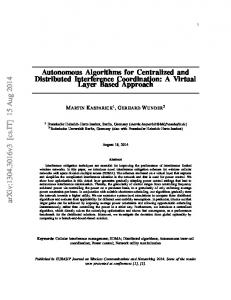
The design of the centralized fault identification scheme that we outlined in the previous section may be difficult to implement in large systems due to communication constraints or overheads. In order to avoid these problems and develop scalable fault identification schemes, we present in this section a distributed fault identification scheme. For simplicity, we first consider a Petri net which can be conveniently decomposed into two interacting sub-
16
systems,4 such as the one shown in Figure 1, where place Ps is shared by subsystems S1 and S2 . For the time being, we assign the shared place to subsystem S2 and design a redundant Petri net embedding for each of the two subsystems separately, utilizing our development in Section IV (refer to Figure 2). Clearly, when a transition associated with the shared place Ps fires in subsystem S1 , the fault identification mechanism for subsystem S2 will treat the result as a place fault in the shared place. One way to overcome this limitation is to compensate the fault syndrome of subsystem S2 by appropriately adjusting the number of tokens in the additional places of S 2 , i.e., by adding arcs between the transitions of S1 that are associated with Ps and the additional places of the redundant embedding for subsystem S2 . More specifically, we need to consider two cases: (i) When the firing of a transition in subsystem S1 generates tokens in the places of subsystem S2 , the fault (2)
(2)
syndrome seen by the fault identification mechanism of S2 is sP = −C(2)∗ eP (superscript (i) is used to denote (2)
subsystem Si and superscript ∗ follows the design in Section IV.C). Here, eP is the additive vector that describes (2)
how the number of tokens in the (original) places of subsystem S2 has been corrupted (i.e., eP is of dimension (2)
n2 as opposed to η2 ). We can account for the erroneous syndrome sP
if we add crossing (output) arcs from
the transition of S1 to the additional places of the redundant embedding for S2 and choose the arc weights to be (2)
(2)
w(2)+ = C(2)∗ eP (note that eP has nonnegative entries, resulting in a nonnegative vector w (2)+ ). With this choice, the resulting syndrome in S2 is zero, i.e., (2) Pqf [t]
=
(2) [−C(2)∗ Id ] qh [t] (2)
= −C(2)∗ eP + w(2)+
+
(2)
eP
0
+
0 w(2)+
=0.
(37)
(ii) When the firing of a transition in subsystem S1 consumes tokens from places of subsystem S2 , causing the fault (2)
(2)
syndrome to be sP = −C(2)∗ eP in S2 , then we need to add crossing (input) arcs from the additional places of (2)
the redundant embedding for S2 to this transition and choose the arc weights to be w (2)− = −C(2)∗ eP (note that (2)
eP has nonpositive entries, resulting in a nonnegative vector w (2)− ). We note that this case may lead to negative values for the total number of tokens in the additional places. If this needs to be avoided, we can artificially add a sufficiently large number of tokens to each additional place and ignore this extra number of tokens when performing parity checks (see the discussion in Section IV.C). We highlight that this compensation method ensures that transition faults in a particular subsystem do not affect fault detection and identification in other subsystems. For instance, in case (i), if a post-condition fault occurs to the transition of S1 that is connected to Ps (in the forward direction), then no tokens are deposited at the shared places or the additional places in S2 . Likewise, in case (ii), if a pre-condition fault occurs to the transition in S1 that is connected to Ps (in the backward direction), there is no effect on S2 . Finally, we note that the value of the prime number p, and accordingly the arc weights and the number of tokens in the additional places, can be significantly reduced with modular designs because they can be confined to a subsystem rather than the entire system. More generally, when multiple subsystems exist in the modular decomposition of a large system, we can imple4 This
can be done in many ways; see, for example, [34, 35] and references therein.
17
ment the above compensation approach in a pairwise fashion. More specifically, given a decomposition of a Petri net into subsystems, we can follow the above approach to build crossing arcs for each pair of subsystems that share one or more places. This is described in the following procedure.
Construction of Distributed Redundant Embeddings: For each subsystem Si , perform the following: 1. Establish an appropriate redundant embedding for Si . 2. For each subsystem Sj , j 6= i, with transitions that connect to or from place(s) in Si , do: (i) For each transition in subsystem Sj with output arc(s) to the shared place(s), build output crossing arcs from this transition to the additional places of the redundant embedding for S i . (ii) For each transition in subsystem Sj with input arc(s) from the shared place(s), build input crossing arcs from the additional places of the redundant embedding for Si to this transition. Note that if one is interested in designing distributed monitoring schemes that minimize the number of crossing arcs, then one can employ several strategies to allocate shared places to subsystems. For example, if all redundant embeddings have the same number of additional places, then, in order to minimize the number of crossing arcs between different subsystems, a shared place should be allocated to the subsystem which has the most arcs connected to that place (each such arc is connected to a transition which is in turn connected via crossing arcs with all additional places). If the embeddings of different subsystems have different number of places, then the shared place should be allocated to the subsystem that is associated with the largest product of number of additional places multiplied by the number of arcs linked to the shared place. The proposed distributed fault identification scheme exhibits great flexibility in terms of scalability. More specifically, when a new subsystem SN is added to an existing system S consisting of subsystems {S1 , S2 , ..., SN −1 }, we can follow the procedure below to upgrade the distributed redundant embeddings. System Upgrade: 1. Establish an appropriate redundant embedding for subsystem SN . 2. For each subsystem Si , 1 ≤ i ≤ N − 1, with transitions that connect to place(s) in SN , do: (i) For each transition in subsystem Si with output arc(s) to place(s) in SN , build output crossing arcs from this transition to the additional places of the redundant embedding for S N . (ii) For each transition in subsystem Si with input arc(s) from place(s) in SN , build input crossing arcs from the additional places of the redundant embedding for SN to this transition. 3. For each subsystem Si which contains place(s) connecting to transitions in SN , do: (i) For each transition in subsystem SN with output arc(s) to the shared place(s), build output crossing arcs from this transition to the additional places of the redundant embedding for S i . (ii) For each transition in subsystem SN with input arc(s) from the shared place(s), build input crossing arcs from the additional places of the redundant embedding for SN to this transition.
18
P1
.
P15
P13
.
P17
T1 P2
.
P9 T9
P18
P16
P10
T2
T10
P3
P11
T3
T11
P4
P12
T4
P14
P5
T12
P6
T5
. T6
P7
T7
P8
T8
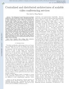
Figure 3: Petri net model of a manufacturing system with three machines and three robots. Note that, since each subsystem is designed to enable the identification of faults independently, the distributed scheme will in general require more additional places and exhibit superior diagnosis capabilities in comparison to the centralized fault identification scheme.
Example
VI
In this section we design centralized and distributed fault identification schemes for the Petri net system shown in Figure 3. This Petri net was studied in [36] and represents the control logic for three machines and three robots as follows: • Machine A(P1 , P2 , P3 , P4 , P13 ; T1 , T2 , T3 , T4 ) consists of places P1 , P2 , P3 , P4 , P13 and transitions T1 , T2 , T3 , T4 ; • Machine B(P5 , P6 , P7 , P8 , P14 ; T5 , T6 , T7 , T8 ) consists of places P5 , P6 , P7 , P8 , P14 and transitions T5 , T6 , T7 , T8 ; • Machine C(P9 , P10 , P11 , P12 , P15 ;
T9 , T10 , T11 , T12 ) consists of places P9 , P10 , P11 , P12 , P15 and transitions
T9 , T10 , T11 , T12 ; • Robots R1 (P16 ), R2 (P17 ), R3 (P18 ). In total, there are twelve transitions (i.e., m = 12) and eighteen places (i.e., n = 18). The initial marking of the Petri net, as indicated in Figure 3 by the number of tokens in each place, is qs [0] = (1 0 0 0 0 0 1 0 1 0 0 0 0 0 0 0 1 0)T 19
and the arc matrices B+ and B− in Eq. (1) are given by
B+ =
0 1 0 0 0 0 0 0 0 0 0 0 0 0 0 0 0 0
0 0 1 0 0 0 0 0 0 0 0 0 0 0 0 0 0 0
0 0 0 1 0 0 0 0 0 0 0 0 0 0 1 1 1 0
1 0 0 0 0 0 0 0 0 0 0 0 0 0 0 0 0 0
0 0 0 0 0 1 0 0 0 0 0 0 0 0 0 0 0 0
0 0 0 0 0 0 1 0 0 0 0 0 0 0 0 0 0 0
0 0 0 0 0 0 0 1 0 0 0 0 1 0 0 1 0 1
0 0 0 0 1 0 0 0 0 0 0 0 0 0 0 0 0 0
0 0 0 0 0 0 0 0 0 1 0 0 0 0 0 0 0 0
0 0 0 0 0 0 0 0 0 0 1 0 0 0 0 0 0 0
0 0 0 0 0 0 0 0 0 0 0 1 0 1 0 0 1 1
0 0 0 0 0 0 0 0 1 0 0 0 0 0 0 0 0 0
B− =
,
1 0 0 0 0 0 0 0 0 0 0 0 1 0 0 1 0 0
0 1 0 0 0 0 0 0 0 0 0 0 0 0 0 0 1 0
0 0 1 0 0 0 0 0 0 0 0 0 0 0 0 0 0 0
0 0 0 1 0 0 0 0 0 0 0 0 0 0 0 0 0 0
0 0 0 0 1 0 0 0 0 0 0 0 0 1 0 0 0 1
0 0 0 0 0 1 0 0 0 0 0 0 0 0 0 1 0 0
0 0 0 0 0 0 1 0 0 0 0 0 0 0 0 0 0 0
0 0 0 0 0 0 0 1 0 0 0 0 0 0 0 0 0 0
0 0 0 0 0 0 0 0 1 0 0 0 0 0 1 0 1 0
0 0 0 0 0 0 0 0 0 1 0 0 0 0 0 0 0 1
0 0 0 0 0 0 0 0 0 0 1 0 0 0 0 0 0 0
0 0 0 0 0 0 0 0 0 0 0 1 0 0 0 0 0 0
.
Centralized Fault Identification: We first describe a centralized fault identification scheme in which we aim to simultaneously detect and identify two transition faults and one place fault. We assume that the number of erroneous tokens in any place is bounded by [−5, 5]. From our development in Section III, we need two additional places (d = 2) and, since the smallest prime number that is greater than both m = 12 and η = 18 + 2 = 20 is 23, we set p = 23. Following the construction in Section IV.C, we choose D∗ so that
D∗ = −23 ×
=
1
2
3
4
5
6
7
8
9
10
11
12
12
22
32
42
52
62
72
82
92
102
112
122
(mod 23)
−23
−46
−69
−92
−115
−138
−161
−184
−207
−230
−253
−276
−23
−92
−207
−368
−46
−299
−69
−414
−276
−184
−138
−138
.
˜ of the Reed-Solomon code can be Since 5 is a primitive element in GF(23), the punctured parity check matrix H chosen (modulo 23) as
˜ ≡ H
1
5
52
53
54
55
56
57
58
59
510
511
512
513
514
515
516
517
518
519
1
52
54
56
58
510
512
514
516
518
520
522
524
526
528
530
532
534
536
538
(mod 23) 1 5 2 10 4 20 8 17 16 11 9 22 18 21 13 19 3 15 6 7 ≡ 1 2 4 8 16 9 18 13 3 6 12 1 2 4 8 16 9 18 13 3 6 7 1 17 17 18 2 18 14 10 22 8 20 14 13 20 10 8 ≡ 13 3 19 19 12 9 12 17 22 7 13 21 17 1 21 22 13 9 | {z }| {z Φ
[C I]
20
2
3
1
0
2
16
0
1
. }
According to our design rule in Eq. (33), we have
C∗ = 23 · 1 −
=
1
17
17
18
2
18
14
10
22
8
20
14
13
20
10
8
2
3
19
19
12
9
12
17
22
7
13
21
17
1
21
22
13
9
2
16
22
6
6
5
21
5
9
13
1
15
3
9
10
3
13
15
21
20
4
4
11
14
11
6
1
16
10
2
6
22
2
1
10
14
21
7
.
Thus, the arc weights to (from) the additional places from (to) the transitions in the original system (shown in Figure 4 with dotted arcs) are given by
C∗ B + − D ∗ = and
C∗ B − − D ∗ =
29
52
123
114
120
147
219
205
222
233
306
277
27
103
266
372
52
300
108
425
278
190
189
148
70
73
75
97
159
158
170
197
242
265
256
285
43
117
218
382
65
319
70
430
317
193
144
160
.
Furthermore, the initial marking of the overall system is
qh [0] =
I18 C∗
qs [0]
= (1 0 0 0 0 0 1 0 1 0 0 0 0 0 0 0 1 0 53 36)T .
(Note that the two additional places are initialized so that the encoded state q h [0] satisfies the parity check [−C∗ I2 ]qh [0] = 0 in GF(23).) According to our choice of D∗ and C∗ , the system is expected to simultaneously detect and identify two transition faults and one place fault. We now check this capability by following a specific example. We assume that the applied firing sequence is T7 , T1 , T2 , T8 , T3 , T9 , and that the following faults occur: a pre-condition fault in transition T2 (during time epoch 3), a place fault that corrupts the number of tokens in P 7 by +2 (during time epoch 5), and a post-condition fault in transition T9 (during time epoch 6). The sequence of markings is given by T7 : qf [1] = (1 0 0 0 0 0 0 1 1 0 0 0 1 0 0 1 1 1
74)T ,
102
T
T1 : qf [2] = (0 1 0 0 0 0 0 1 1 0 0 0 0 0 0 0 1 1
61
58) ,
T2 : qf [3] = (0 1 1 0 0 0 0 1 1 0 0 0 0 0 0 0 1 1
113
161)T , T
Fault-free Fault-free Pre-condition fault in T2
T8 : qf [4] = (0 1 1 0 1 0 0 0 1 0 0 0 0 0 0 0 1 1
121
156) ,
Fault-free
T3 : qf [5] = (0 1 0 1 1 0 2 0 1 0 0 0 0 0 1 1 2 1
169
204)T ,
P7 corrupted by + 2
T9 : qf [6] = (0 1 0 1 1 0 2 0 0 0 0 0 0 0 0 1 1 1
−73
T
−113) ,
Post-condition fault in T9
where the indication on the right refers only to fault events during the corresponding time epoch. The resulting syndrome at time epoch t = 6 is
s[6] = [−C∗ I2 ]qf [6] =
−179 −186
21
≡
5 21
(mod 23) .
P1
.
P15
P13
.
P17
T1 P2
.
P9 T9 P10
P18
P16
T2
T10
P3
P11
T3
T11
P4
P12 P14
T4
P5
T12
T5
P6
. T6
P7
P8
T7
T8
Figure 4: Centralized fault detection and identification for the manufacturing system of Figure 3 using a redundant Petri net embedding. We proceed to identify the faults. First, by left multiplying by Φ, we obtain the modified place fault syndrome
s0P = Φs[6] (mod 23) ≡
6
7
13
3
5 21
=
16 13
.
˜ we easily identify place P7 as faulty with the erroneous number By inspecting the punctured parity check matrix H, ˜ This is consistent with of tokens being +2 (the syndrome s0P is equal to twice the seventh column of matrix H). the faults that took place during the operation of the system. Once place faults have been identified, we utilize (36) to obtain
DeT = −(s[6] − P∗ eP )/23 =
7 8
.
We note that the above syndrome does not coincide with any column of ±D, so there must be two transition faults (if identifiable). We first consider the case of both faults undergoing pre-condition faults, which results in the following equation array:
−x − x ≡ 7, 1 2 −x2 − x2 ≡ 8 . 1 2
22
By simple calculation, we obtain Λ1 (x1 , x2 ) ≡ −7 and Λ2 (x1 , x2 ) ≡ 11; the corresponding polynomial is x2 − 7x + 11 = 0 but its roots are not proper solutions. Similarly, we eliminate the possibility of both faults being post-condition faults. We then try the case of a pre-condition fault and a post-condition fault, which translates to solving x − x ≡ 7, 1 2 x2 − x2 ≡ 8. 1 2 These equations are easily shown to have a unique solution with x1 = 9 and x2 = 2. Therefore, we conclude that transition T2 suffered a pre-condition fault and transition T9 suffered a post-condition fault, which is consistent with the faults that took place during the operation of the system. The simplified identification procedures presented above can be done systematically (using the procedure in Section IV.A for the identification of transition faults and the Berlekamp-Massey algorithm for the identification of place faults). Note that, during the operation of the redundant Petri net system in our example, the number of tokens in the additional places becomes negative (at time epoch 6). If the additional places function as controllers (as in [29, 30]), then this implies that the firing of transition T9 during time epoch 6 would be inhibited. If this is the case, this problem can be avoided by adding a sufficiently large number of extra tokens to each additional place (and ignoring this extra number of tokens when performing parity checks). For example, if we add 500 tokens to each additional place, the state evolution of the redundant Petri net would appear as T7 : qf [1] = (1 0 0 0 0 0 0 1 1 0 0 0 1 0 0 1 1 1
500 + 102
500 + 74)T ,
Fault-free
T1 : qf [2] = (0 1 0 0 0 0 0 1 1 0 0 0 0 0 0 0 1 1
500 + 61
500 + 58)T ,
Fault-free
T2 : qf [3] = (0 1 1 0 0 0 0 1 1 0 0 0 0 0 0 0 1 1
500 + 113
500 + 161)T ,
Pre-condition fault in T2
T
T8 : qf [4] = (0 1 1 0 1 0 0 0 1 0 0 0 0 0 0 0 1 1
500 + 121
500 + 156) ,
Fault-free
T3 : qf [5] = (0 1 0 1 1 0 2 0 1 0 0 0 0 0 1 1 2 1
500 + 169
500 + 204)T ,
P7 corrupted by + 2
T9 : qf [6] = (0 1 0 1 1 0 2 0 0 0 0 0 0 0 0 1 1 1
500 − 73
T
500 − 113) ,
Post-condition fault in T9
and detection and identification would progress in exactly the same way as before, given that the 500 added tokens in the additional places are ignored when performing parity check calculations. Distributed Fault Identification: We now discuss a distributed fault identification scheme for the Petri net in
Figure 3. We find it convenient to decompose the system into three subsystems: subsystem S 1 (P1 , P2 , P3 , P4 , P13 , P16 ; T1 , T2 , T3 , T4 subsystem S2 (P5 , P6 , P7 , P8 , P14 , P18 ; T5 , T6 , T7 , T8 ) and subsystem S3 (P9 , P10 , P11 , P12 , P15 , P17 , T9 , T10 , T11 , T12 ). Since the sole difference between the three subsystems is their initial marking, we only discuss the design of the monitor for subsystem S1 with places P13 and P16 shared between subsystems S1 and S2 . As in the centralized case, our objective is to detect and identify up to one place fault and/or up to two transition faults so that the number of additional places is given by di = 2 for each subsystem Si . As before, we allow place faults to add an erroneous number of tokens within [−5, 5]. Since the smallest qualified prime number is p = 11 (note that in this
23
case p = 11 is greater than both mi = 4 and ηi = ni + di = 8 for each subsystem Si ), we can adopt D(1)∗ such that
D(1)∗ = −11 ·
=
1
2
3
4
12
22
32
42
−11
−22
−33
−44
−11
−44
−99
−55
(mod 11)
.
˜ is given by Since 2 is a primitive element in GF(11), the punctured parity check matrix H
1
˜ = H
=
=
2
4
2
5
2
6
2
8
2
10
1
2
1
2
8
5
10
9
7
1
4
5 9
3
1
4
5
9
7
4
5
2
{z
|
2
3
2
C(1)∗ = 11 · 1 −
2
4
4
7
8
3
10
1
3
2
6
2
12
214
2
9
}|
Φ
thus, we have
2
2
7
(mod 11)
8
9
1
0
10 3 {z
4
0
1
8
3
9
8
9
10
1
3
10
3
4
; }
[C I]
7
=
4
3
8
2
3
2
1
10
8
1
8
7
and the two directed weight matrices in the embedded subsystem are given by
B
(1)+
C(1)∗ B(1)+ − D(1)∗
0
0
0
1
1 0 0 0 0 1 0 0 0 0 1 0 = , 0 0 0 0 0 0 1 0 14 30 37 48 21 52 107 56
B
(1)−
C(1)∗ B(1)− − D(1)∗
=
1
0
0
0
1
0
0
0
1
0
0
0
1
0
0
1
0
0
20
25
41
27
54
107
0
0 0 1 . 0 0 46 56
If transition T7 (in S2 ) fires, it produces one token in each of P13 and P16 . From the perspective of subsystem S1 , this is regarded as a (multiple) place fault. To balance the syndrome, the crossing arc weights from T 7 to the additional places of S1 are set to be (1)+
w7
= C(1)∗ · (0 0 0 0 1 1)T =
24
5 15
.
P1
.
P15
P13
.
P17
T1 P2
S1
.
P9 T9 P10
P18
P16
T2
T10
P3
P11
T3
T11
P4
P12
T4
P14
P5
S3
T12
T5
P6
. T6
P7
T7
P8
T8
S2 Figure 5: Distributed fault identification scheme for the system depicted in Figure 3. If transition T6 (in S2 ) fires, it consumes one token from place P16 . The syndrome for S1 can be balanced by setting the crossing arc weights from the additional places of S1 to transition T6 to be (1)−
w6
= −C(1)∗ · (0 0 0 0 0 − 1)T =
2 7
.
The resulting distributed identification scheme (for all three subsystems and monitors) is illustrated in Figure 5, where P13 and P16 in S1 are shared with S2 , P14 and P18 in S2 are shared with S3 , and P15 and P17 in S3 are shared with S1 . As expected, the connecting structure of Figure 5 exhibits a more distributed nature than the structure of Figure 4. To illustrate the capabilities of the resulting distributed identification scheme, we present a more complicated event sequence and show the identification procedure that occurs in subsystem S 1 . The initial marking of the redundant embedding of subsystem S1 is (1)
qh [0] =
I6 C(1)∗
q(1) s [0]
= (1 0 0 0 0 0 4 1)T .
25
Let the sequence of markings within subsystem S1 be as follows: (1)
T7 :
qf [1]
T1 :
(1) qf [2] (1) qf [3] (1) qf [4] (1) qf [5] (1) qf [6] (1) qf [7] (1) qf [8] (1) qf [9] (1) qf [10] (1) qf [11] (1) qf [12]
T2 : T3 : T4 : T9 : T10 : T11 : T8 : T5 : T6 : T7 :
= (1 0 0 0 1 1
16)T ,
9
T
Fault-free
= (0 1 0 0 0 0
3
10) ,
Fault-free
= (0 1 1 0 0 0
33
62)T ,
Pre-condition fault in T2
T
= (0 1 0 3 0 1
29
62) ,
= (0 1 0 2 0 1
−17
6)T ,
Post-condition fault in T4
= (0 1 0 2 0 1
−17
6)T ,
Fault-free
= (0 1 0 2 0 1
−17
T
6) ,
Pre-condition fault in T10
= (0 1 0 2 0 1
−17
6)T ,
Fault-free
= (0 1 0 2 0 1
−17
T
6) ,
Fault-free
= (0 1 0 2 0 1
−17
6)T ,
Fault-free
= (0 1 0 2 0 0
−19
−1)T ,
Fault-free
= (0 1 0 2 0 0
T
−19
−1) ,
P4 corrupted by + 2
Post-condition fault in T7
(again, if desired/necessary, we can add tokens to each additional place to ensure that the number of tokens in the additional places does not become negative and inhibit transitions that would otherwise be enabled in the original Petri net). Let us assume that we perform a non-concurrent check at time epoch 12. We first compute the resulting syndrome
(1)
s[12] = [−C(1)∗ I2 ] qf [12] =
−26 −13
≡
7 9
.
Thus, faults have been successfully detected. Left multiplying by Φ and taking the result modulo p = 11, we obtain the following parity check equation
|
9
7
4
5 {z Φ
}
7 9
≡
5 7
≡
1
2
4
8
5
10
9
7
1
4
5
9
3 {z
1
4
5
|
eP . }
˜ H
By inspection, we obtain eP = [0 0 0 2 0 0]T , which agrees with the faults that took place in the system. ¿From Eq. (36), the transition fault syndrome is given by
DeT = −(s[12] − P∗ eP )/11 =
2 1
and, since it does not coincide with any column of D(1)∗ , we conclude that there must be two transition faults (if identifiable). We first consider the case of both faults being post-condition faults, which results in the following equation array:
x + x ≡ 2, 1 2 x2 + x2 ≡ 1. 1 2
26
By simple calculation, we obtain Λ1 (x1 , x2 ) ≡ 2 and Λ2 (x1 , x2 ) ≡ 7; the corresponding polynomial is x2 + 2x + 7 ≡ 0 and has roots 3 and 6. However, since 6 is not a valid index for a transition in this subsystem, this is an invalid solution. Similarly, we eliminate the possibility of both faults being pre-condition faults. We then try the case of a pre-condition fault and a post-condition fault, which results in the following equation array: x − x ≡ 2, 1 2 x2 − x2 ≡ 1. 2 1 This equation is easily shown to have a unique solution x1 = 4 and x2 = 2. Therefore, we conclude that transition T2 suffered a pre-condition fault and transition T4 suffered a post-condition fault, which is consistent with the faults that took place during the operation of the system. Note that faults in other subsystems (namely the pre-condition fault in transition T 10 ) do not affect fault identification in subsystem S1 . Moreover, our design for subsystem S1 is shown to be immune to the post-condition fault in transition T7 .
VII
Conclusions and Future Work
In this paper we have presented centralized and distributed fault identification schemes for discrete event systems that are described by Petri nets. Our setting assumes that system events (transition firings) are not directly observable but that the system state (marking) is periodically observable, and aims at capturing faults in both Petri net transitions and places. To achieve this, we introduce redundancy and construct a redundant Petri net embedding whose additional places encode information in a way that enables error detection and identification to be performed using algebraic decoding techniques. Our approach does not need to reconstruct the various possible state evolution paths associated with a given DES and has small identification overhead. More specifically, using 2k additional places (and the connections and tokens associated with them), the proposed scheme can simultaneously identify 2k − 1 transition faults and k place faults that may take place in the system. The worst-case complexity of the fault identification procedure is O(k(m + n)) operations, where m and n are respectively the number of transitions and places in the given Petri net. The proposed fault identification scheme was also modified to accommodate distributivity in a way that requires little additional hardware. Our current work focuses on understanding ways to introduce redundancy so that we minimize the number of additional connections (as opposed to the number of additional places). More generally, we are interested in developing low-complexity identification schemes that minimize cost functions associated with the additional places and/or connections, in both centralized and distributed settings. Another interesting future direction is to generalize the techniques introduced in this paper to settings where certain Petri net places and/or transitions are unobservable or partially observable.
27
References [1] J. Gertler, Fault Detection and Diagnosis in Engineering Systems. Marcel Dekker, New York, 1998. [2] E. Y. Chow and A. S. Willsky, “Analytical redundancy and the design of robust failure detection systems,” IEEE Trans. Automatic Control, vol. 29, pp. 603–614, July 1984. [3] C. N. Hadjicostis and G. C. Verghese, “Monitoring discrete event systems using Petri net embeddings,” Application and Theory of Petri Nets 1999 (Series Lecture Notes in Computer Science, vol. 1639), pp. 188–207, 1999. [4] R. E. Blahut, Algebraic Codes for Data Transmission, Cambridge University Press, Cambridge, UK, 2002. [5] S. B. Wicker, Error Control Systems, Prentice Hall, Englewood Cliffs, New Jersey, 1995. [6] Y. Wu and C. N. Hadjicostis, “On solving composite power polynomial equations.” Submitted to Mathematics of Computation. [7] Y. Wu and C. N. Hadjicostis, “Non-concurrent fault identification in discrete event systems using encoded Petri net states,” in Proc. of the 41st IEEE Conf. on Decision and Control, pp. 4018–4023, 2002. [8] M. Sampath, R. Sengupta, S. Lafortune, K. Sinnamohideen, and D. Teneketzis, “Diagnosability of discreteevent systems,” IEEE Trans. Automatic Control, vol. 40, pp. 1555–1575, Sept. 1995. [9] M. Sampath, R. Sengupta, S. Lafortune, K. Sinnamohideen, and D. Teneketzis, “Failure diagnosis using discrete-event models,” IEEE Trans. Control System Technology, vol. 4, pp. 105–124, March 1996. [10] M. Sampath, S. Lafortune, and D. Teneketzis, “Active diagnosis of discrete-event systems,” IEEE Trans. Automatic Control, vol. 43, pp. 908–929, July 1998. [11] J. Shengbing and R. Kumar, “Failure diagnosis of discrete event systems with linear-time temporal logic fault specifications,” in Proc. of the 2002 American Control Conference, pp. 128–133, 2002. [12] R. Debouk, S. Lafortune, and D. Teneketzis, “On an optimization problem in sensor selection for failure diagnosis,” in Proc. of the 38th IEEE Conf. on Decision and Control, pp. 4990–4995, 1999. [13] R. Debouk, S. Lafortune, and D. Teneketzis, “On the effect of communication delays in failure diagnosis of decentralized discrete event systems,” in Proc. of the 39th IEEE Conf. on Decision and Control, pp. 2245–2251, 2000. [14] J. Shengbing, R. Kumar, and H. E. Garcia, “Optimal sensor selection for discrete-event systems with partial observation,” IEEE Trans. Automatic Control, vol. 48, pp. 369–381, March 2003. [15] D. N. Pandalai and L. E. Holloway, “Template languages for fault monitoring of timed discrete event processes,” IEEE Trans. Automatic Control, vol. 45, pp. 868–882, May 2000. [16] V. S. Srinivasan and M. A. Jafari, “Fault detection/monitoring using time Petri nets,” IEEE Trans. Syst., Man, & Cybern., vol. 23, pp. 1155–1162, July–Aug. 1993. [17] S. K. Yang and T. S. Liu, “A Petri net approach to early failure detection and isolation for preventive maintenance,” Quality & Reliability Engineering International, vol. 14, pp. 319–330, Sept.–Oct. 1998. [18] C. H. Kuo and H. P. Huang, “Failure modeling and process monitoring for flexible manufacturing systems using colored timed Petri nets,” IEEE Trans. Robotics & Automation, vol. 16, pp. 301–312, June 2000. [19] G. Barrett and S. Lafortune, “Decentralized supervisory control with communicating controllers,” IEEE Trans. Automatic Control, vol. 45, pp. 1620–1638, Sept. 2000. [20] R. K. Boel and J. H. van Schuppen, “Decentralized failure diagnosis for discrete-event systems with costly communication between diagnosers,” in Proc. of the Sixth International Workshop on Discrete Event Systems, pp. 175–181, 2002. [21] R. Sengupta, “Diagnosis and communications in distributed systems,” in Proc. of the International Workshop on Discrete Event Systems, pp. 144–151, 1998.
28
[22] R. Debouk, S. Lafortune, and D. Teneketzis, “Coordinated decentralized protocols for failure diagnosis of discrete event systems,” Discrete Event Dynamic Systems: Theory and Application, vol. 10, pp. 33–86, Jan. 2000. [23] A. Benveniste, E. Fabre, C. Jard, and S. Haar, “Diagnosis of asynchronous discrete event systems: a net unfolding approach,” IEEE Trans. Automatic Control, vol. 48, pp. 714–727, May 2003. [24] A. Aghasaryaiu, E. Fabre, A. Benveniste, R. Boubour, and C. Jard, “Fault detection and diagnosis in distributed systems: an approach by partially stochastic Petri nets,” Discrete Event Dynamic Systems: Theory and Applications, vol. 8, pp. 203–231, June 1998. [25] P. Baroni, G. Lamperti, P. Pogliano, and M. Zanella, “Diagnosis of a class of distributed discrete-event systems,” IEEE Trans. Syst., Man, & Cybern. Part A: Systems & Humans, vol. 30, pp. 731–752, Nov. 2000. [26] A. Giua and C. Seatzu, “Observability of place/transition nets,” IEEE Trans. Automatic Control, vol. 47, pp. 1424–1437, Sept. 2002. [27] Y. Li and W. M. Wonham, “Control of vector discrete-event systems — Part I: the base model,” IEEE Trans. Automatic Control, vol. 38, pp. 1214–1227, Aug. 1993. [28] Y. Li and W. M. Wonham, “Control of vector discrete-event systems — Part II: controller synthesis,” IEEE Trans. Automatic Control, vol. 39, pp. 512–531, March 1994. [29] K. Yamalidou, J. Moody, M. Lemmon and P. Antsaklis, “Feedback control of Petri nets based on place invariants,” Automatica, vol. 32, pp. 15–28, Jan. 1996. [30] J. O. Moody and P. J. Antsaklis, “Petri net supervisors for DES with uncontrollable and unobservable transitions, IEEE Trans. Automatic Control, vol. 45, pp. 462–476, March 2000. [31] C. G. Cassandras and S. Lafortune, Introduction to Discrete Event Systems, Kluwer Academic Publishers, Boston, MA, 1999. [32] T. Murata, “Petri nets: properties, analysis and applications,” Proc. of the IEEE, vol. 77, pp. 541–580, April 1989. [33] J. Riordan, An Introduction to Combinatorial Analysis, John Wiley & Sons, New York, 1958. [34] A. Aybar and A. Iftar, “Overlapping decompositions and expansions of Petri nets,” IEEE Trans. Automatic Control, vol. 47, pp. 511–515, March 2002. [35] S. Christensen and L. Petrucci, “Modular analysis of Petri nets,” The Computer Journal, vol. 43, pp. 224–242, March 2000. [36] R. Y. Al-Jaar and A. A. Desrochers, “Petri nets in automation and manufacturing,” Advances in Automation and Robotics, G. N. Saridis, Ed., vol. 2, JAI Press, Greenwich, CT, 1990.
29