Detection with distributed sensors has been studied for nearly three decades .... With the PDF of the GLRT test statistic of (3), we now show the performance of ...
1
On Centralized Composite Detection with Distributed Sensors Cuichun Xu, and Steven Kay
Abstract For composite hypothesis testing, the generalized likelihood ratio test (GLRT) and the Bayesian approach are two widely used methods. This paper investigates the two methods for signal detection of a known waveform and unknown amplitude with distributed sensors. It is first proved that the performance of GLRT can be poor and hence improved for this problem and then an approximated Bayesian detector is proposed. Compared with the exact Bayesian approach, the proposed method always has a closed form and hence is easy to implement. Computer simulation results show that the proposed method has comparable performance to the exact Bayesian approach.
I. I NTRODUCTION Detection with distributed sensors has been studied for nearly three decades [1] [2] [3]. With respect to different data assumptions, it can be categorized to centralized detection and decentralized detection. In centralized detection, it is assumed that all data from all local sensors are available for processing. In decentralized detection, only compressed data or local decision from all local sensors are communicated to a central processor, where a central decision is made. Since the centralized detection can largely resort to classical detection theory, many works focus on decentralized detection [1] [2] [3]. However, there are still some problems left for centralized detection, especially when there are unknown parameters in hypotheses, i.e. composite detection. In [4], a minimax constant false alarm rate (CFAR) centralized detector is proposed for composite detection. However, it assumes that the unknown parameters take discrete values and the detection involves large computation. In [3], many distributed detection techniques are reviewed, with focus on the locally optimum distributed detectors, which are optimal only when signal is weak. Other common composite detection methods include the generalized likelihood ratio test (GLRT) and the Bayesian approach. Because of its ease of implementation, the GLRT is widely used and usually has satisfactory performance. However, its optimality is hard to establish, even though some attempts have been made, based
2
on different criteria [8] [9]. On the other hand, the Bayesian approach is optimal if the assumed prior probabilities and prior probability density functions (PDFs) of the unknown parameters are true. However, in most applications the true priors and true prior PDFs are unknown and hard to assume. Furthermore the integration involved in calculation of the marginal PDF may not be easy to evaluate [12]. In this paper, we examine the important special case of independent sensors (conditioned on hypothesis). In particular, we focus on situations that even when a signal is present only part of the sensors receive the signal. It is shown in Section III that in this case, the GLRT is not optimal. Some improvements of the GLRT are also discussed. In section IV, an approximated Bayesian detector is proposed based on vague prior PDFs, which does not need a specific form. Some computer simulation results are shown in Section V and finally Section VI offers conclusion and further discussion. II. S TATEMENT
OF THE
P ROBLEM
To simplify the mathematical exposition, we assume the sensors are ordered with respect to their importance. That is if i ≤ j and sensor j receives signal then sensor i must also receive signal. This order of importance may be due to the physical locations of the sensors. When the sensors are not ordered, the discussion is given in Section VI. We assume that there are M independent sensors or channels. The detection problem is stated as H0 : x [n] = w [n]
n = 0, 1, · · · , N − 1
(1)
H1 : x [n] = As [n] + w [n] n = 0, 1, · · · , N − 1
where A is the M × 1 unknown amplitude vector, with possibly different elements, s[n] is a known waveform and w[n] is a Gaussian random vector. Each element of w[n] is white both in time domain and in space domain, i.e. E [wi [n] wi [m]] =
and E [wi [n] wj [n]] =
σ2, 0,
n=m n 6= m
σ2, i = j 0,
i 6= j
for any 1 ≤ i ≤ M
for any 0 ≤ n ≤ N − 1
where wi [n] denotes the ith element of w[n] and E[·] denotes the expectation operator. Since the sensors are ordered, under H1 only the first L elements of A is nonzero. L is referred to as the true model order under H1 . Both L and the value of the first L elements of A are unknown. If we assume there are i nonzero elements in A, the corresponding model of (1) is called model i and is denoted as Mi . Under
3
model Mi , A is denoted as Ai and Ai = [A1 , A2 , · · · , Ai , 0, 0, · · · , 0]M ×1 Clearly, under H0 the data is from model M0 and under H1 the data is from model Mi , 1 ≤ i ≤ M . With this modeling, the detection problem can equivalently be stated as to assign the given data to M0 (H0 ) or to M1 ∪ M2 ∪ · · · ∪ MM (H1 ). III. G ENERALIZED L IKELIHOOD R ATIO T EST A. Performance of the GLRT Firstly, suppose the variance σ 2 is known. Since L and A are unknown, the GLRT decides H1 if LG (X) = max
�
ˆ i , Mi p X; A p (X; M0 )
1≤i≤M
�
>λ �
ˆ i , Mi where X = [x[0], x[1], · · · , x[N − 1]]T denotes the whole data and p X; A
�
is the probability
ˆ i , which density function (PDF) under Mi parameterized by the maximum likelihood estimator (MLE) A
is estimated assuming Mi is true. Since if i ≤ j , Mi can be thought of as a special case of Mj , it is readily shown that the GLRT will always implement the test statistic based on the maximum model, i.e. [5] LG (X) =
�
ˆ M , MM p X; A p (X; M0 )
or equivalently 2 ln LG (X) = 2 ln
�
�
>λ
ˆ M , MM p X; A p (X; M0 )
�
> λ′
(2)
The test statistic of (2) has the PDF [5] 2 ln LG (X) ∼
χ2 , M
H0
χ′2 (λ) , H1 M 2
(3)
where χ2M denotes the chi-squared distribution and χ′M (λ) denotes the noncentral chi-squared distribution with the noncentrality parameter λ. The noncentrality parameter is given by ε
ε=
A2i
i=1 σ2
λ=
where
M P
N −1 X
s2 [n]
n=0
is the signal waveform energy. Since only the first L elements of A are nonzero, we have ε λ=
L P
A2i
i=1 σ2
4
With the PDF of the GLRT test statistic of (3), we now show the performance of the GLRT is generally not optimal and can be improved. Suppose L < M and let K be an integer such that L ≤ K < M . If there is a generalized likelihood ratio test based on MK , which decides H1 if 2 ln LGK (X) = 2 ln
�
ˆ K , Mk p X; A p (X; M0 )
�
> λ′′
(4)
the PDF of this test statistic is given by 2 ln LGK (X) ∼
χ2 , K
H0
χ′2 (λ) , K
(5)
H1
We note that if the variance σ 2 is unknown, (2) and (4) should be changed to 2 ln LG (X) = 2 ln
�
2 ,M ˆ M, σ p X; A ˆM M
and 2 ln LGK (X) = 2 ln
p X; σ ˆ02 , M0
�
�
2 ,M ˆ K, σ p X; A ˆK K
p X; σ ˆ02 , M0
�
�
> λ′
�
> λ′′
where σ ˆi2 is the MLE of σ 2 under Mi . However, asymptotically (3) and (5) still hold [5]. Since K < M , from Theorem 1, which is proved in Appendix I, the detector based on model MK has better performance than that of the GLRT, which is based on MM . Theorem 3.1: Suppose there are two detection statistics T1 and T2 . The detection statistic T1 has the PDF T1 ∼
χ2 , ν1 2
χ′ν1 (λ) ,
H0 H1
and the detector 1 decides a signal is present if T1 > γ1 . The detection statistic T2 has the PDF T2 ∼
χ2 , ν2
2 χ′ν2 (λ) ,
H0 H1
and the detector 2 decides a signal is present if T2 > γ2 . Then, if ν1 < ν2, the performance of detector 1 is better than that of detector 2 in a Neyman-Pearson (NP) sense, i.e. for the same false alarm rate detector 1 has a higher probability of detection than detector 2. In other words, for this distributed detection problem, if L < M the GLRT is not optimal. This is because the GLRT is based on MM and therefore the channels that contain only noise samples are included in the test statistic. Including these channels will increase the degrees of freedom of the test statistic, however the noncentrality parameter remains the same.
5
B. Improved GLRT From Theorem 1, any detector based on Mi with i > L will have a performance less than the detector based on ML . It is clear that the unknown order L is critical to the performance of detectors. In order to
ˆ can improve the GLRT, L can first be estimated and a generalized likelihood ratio test based on model L
then be conducted. This can be done by using various model order selection criteria [6]. A widely used criterion is the minimum description length (MDL) criterion, which selects the model that minimizes M DL (i) = −2 ln LGi (X) + i ln N,
1≤i≤M
(6)
The GLRT with estimated model is referred to as “rGLRT” in this paper. Recently, a multifamily likelihood ratio test (MFLRT) is proposed to modify the GLRT to accommodate nested PDF families [7]. The MFLRT decides H1 if TM F LRT (X) = max
1≤i≤M
�
��
LGi (X) − i ln
�
LGi (X) i
�
�� �
+1
u
LGi (X) −1 i
��
>γ
(7)
where u(·) is the unit step function. These two revised GLRTs will be compared with the GLRT in Section V. IV. BAYESIAN A PPROACH A. Approximated Bayesian Approach Firstly, suppose the variance σ 2 is known. If we are willing to assume Bayesian assumptions, that is model Mi , 0 ≤ i ≤ M has a prior probability πi and under each model in H1 , Aj , 1 ≤ j ≤ M has a prior PDF given as p(Aj |Mj ), the optimal NP detector decides H1 if p (X|H1 ) >λ p (X|H0 )
(8)
M X
(9)
From the Bayesian assumptions p (X|H1 ) =
πi p (X|Mi )
i=1
Plugging (9) into (8), the detector decides H1 equivalently if M P
πi p (X|Mi )
i=1
p (X|M0 )
>λ
(10)
where the marginal PDF p(X|Mi ) is given by p (X|Mi ) = =
Z
Z
p (X, Ai |Mi ) dAi p (X|Ai , Mi ) p (Ai |Mi ) dAi
(11)
6
As mentioned previously, the true prior PDFs are usually unknown and hard to assume. Furthermore the integration in (11) may not have a closed form. If the variance σ 2 is unknown should be replaced by
RR
R
p (X|Ai , Mi ) p (Ai |Mi ) dAi
p X|Ai , σ 2 , Mi p Ai , σ 2 |Mi dAi dσ 2 and it is even more difficult to assume �
�
the prior PDFs as well as calculate the integration.
It is shown in [10] that assuming vague prior PDFs, the marginal PDF p(X|Mi ) can be asymptotically approximated as 1
− i ˆ i 2 (2πe) 2 ˆ i , Mi I A p (X|Mi ) ≈ const · p X|A
�
� �
�
�
�
ˆ i is the observed information matrix, or where | · | denotes determinant and I A �
ˆi I A
�
∂ 2 ln p (X|Ai , Mi ) =− ∂Ai ∂ATi ˆ A =A i
i
For the model given by (1), it can be shown that asymptotically � � ˆ I A i ≈ N i
and therefore
�
ˆ i , Mi p (X|Mi ) ≈ const · p X|A
� � N �− 2i
2πe
(12)
Plugging the above into (10) we have M P
i=1
or
�
ˆ i , Mi πi const · p X|A p (X|M0 ) M X
πi
i=1
�
N 2πe
�− i
2
��
N 2πe
�− i
2
> λ′
LGi (X) > λ′′
(13)
When σ 2 is unknown, similarly we have �
ˆ i, σ p (X|Mi ) ≈ const · p X|A ˆi2 , Mi
� � N �− i+1 2
2πe
and (13) is still valid. The detector given by (13) is referred to as “aBayesian” in the simulations of Section V. B. An Exact Bayesian Detector In order to make a comparison to the approximated Bayesian detector in the simulations in Section V, in this subsection we provide a set of Bayesian prior PDFs that result in a detector with a closed form.
7
Suppose σ 2 is known, and under Mi , the i elements of Ai are independent and identically distributed, or p (Ai |Mi ) =
i Y
p (Ak )
(14)
k=1
Assume under any model Mi , 1 ≤ i ≤ M p (Ak ) = q
1 2 2πσA k
!
1 exp − 2 (Ak − µk )2 , 2σAk
1≤k≤i
(15)
Denoting xk = [Xk [0], Xk [1], · · · , Xk [N − 1]]T as the data vector from channel k , because each channel is independent to other channels we have i Y p (X|Mi ) p (xk |Mi ) = p (X|M0 ) k=1 p (xk |M0 )
Denoting
p(xk |Mi ) p(xk |M0 )
(16)
as R (xk ), with the assumed prior PDFs, after some algebra we have
R (xk ) =
s
2 (¯ xk )2 + 2N µk x ¯k σ 2 − N µ2k σ 2 N 2 σA σ2 k � � exp 2 + σ2 N σA 2σ 2 N σ 2 + σ 2 k Ak
(17)
where xk denotes the mean of the data from sensor k , given as x ¯k =
−1 1 NX Xk [n] N n=0
From (10) and (16) the Bayesian detector decides H1 if M X i=1
πi
i Y
R (xk ) > λ
(18)
k=1
V. C OMPUTER S IMULATIONS In this section the previously discussed detectors are compared via computer simulations. We note, these detectors are derived from different origins and have quiet different properties. The performance of each detector requires further investigation. This section only serves to give some examples of these detectors and to show the GLRT can be improved. A. Known Variance Define the SNR of channel k as εA2k SNRk = 10 log 10 σ2
!
With this definition, when SNRk ≥ 20dB all methods yield pretty good results. Therefore the main concern is the situation when SNRk < 20dB, i.e. when |Ak |
0.04. For relatively high SNR case, it can be seen in the Fig. 2 that the GLRT is the worst for all
region of the ROC curve. Comparing Fig. 1 and Fig. 2, it is seen that the aBayesian detector has very similar performance to the exact Bayesian detector. It is also seen from Fig. 1 and Fig. 2, when SNR is low, the rGLRT is close to the GLRT, which is the worst detector, and when SNR is high rGLRT is the best detector. Compared with the rGLRT, the MFLRT is more robust. Actually, it can be shown the MFLRT has some minimax properties, which will be addressed in a future work. B. Unknown Variance When the variance σ 2 is unknown, it can be shown LGi (X) =
σ ˆ02 σ ˆi2
! MN 2
9
ROC curves from 5000 trials; SNR = 6; M = 5 0.9
0.8
PD
0.7
0.6 MFLRT Glrt
0.5
Bayesian aBayesian 0.4
0.3 0
Fig. 1.
rGLRT
0.05
0.1
0.15 PFA
0.2
0.25
0.3
ROC curves of the detectors in relatively low SNR (known variance).
. ROC curves from 5000 trials; SNR = 12; M = 5 1 0.98 0.96 0.94
PD
0.92 MFLRT
0.9
Glrt 0.88
Bayesian aBayesian
0.86
rGLRT
0.84 0.82 0.8 0
0.01
0.02
0.03
0.04
0.05
P
FA
Fig. 2.
ROC curves of the detectors in relatively high SNR (known variance).
.
where
M k −1 X X 1 NX (Xj [n])2 (Xi [n] − x ¯i )2 + σ ˆk2 = N M n=0 i=1 j=k+1
10
Because in this case, it is even more difficult to assume valid prior PDFs, we only compare the other 4 detectors. When SNR= 6 the performances of detectors of 5000 realizations are shown in Fig. 3, and when SNR= 12 the performances of detectors of 5000 realizations are shown in Fig. 4. For relatively ROC curves from 5000 trials; SNR = 6; M = 5 0.9
0.8
PD
0.7
0.6 MFLRT Glrt
0.5
aBayesian rGLRT 0.4
0.3 0
Fig. 3.
0.05
0.1
0.15 PFA
0.2
0.25
0.3
ROC curves of the detectors in relatively low SNR (unknown variance).
. low SNR case, it can be seen in the Fig. 3 that the aBayesian detector and the MFLRT are better than the GLRT for all region of the ROC curve. The rGLRT are better than the GLRT for the region of the ROC curve where PF A > 0.04. For relatively high SNR case, it can be seen in the Fig. 4 that the GLRT is the worst for all region of the ROC curve. The minimax property of the MFLRT can also be observed comparing Fig. 3 and Fig. 4. VI. C ONCLUSIONS
AND
D ISCUSSION
We have investigated the GLRT and the Bayesian approach for centralized composite distributed detection. In particular, In particular, we have proved that the performance of GLRT is poor and can be improved for this problem. An approximated Bayesian detector has also been proposed based on vague prior PDFs, and therefore the marginal PDF can be obtained without integration. As a result, the detector always has a closed form. In our exposition, we assume the sensors have already been ordered with respect to their importance. Therefore when there are M sensors, only M + 1 models need to be considered. When the original data
11
ROC curves from 5000 trials; SNR = 12; M = 5 1 0.98 0.96 0.94
PD
0.92 0.9 MFLRT
0.88
Glrt 0.86
aBayesian rGLRT
0.84 0.82 0.8 0
0.01
0.02
0.03
0.04
0.05
P
FA
Fig. 4.
ROC curves of the detectors in relatively high SNR (unknown variance).
.
from sensors are not ordered, for M sensors we have to consider 2M models as in [4]. This will greatly increase the computational load. Alternatively, some preliminary processing can be conducted to order the sensors and similar techniques as in [11] can be used. However, the performance degradation as a result of ordering needs further investigation. R EFERENCES [1] R. R. Tenney and N. R. Sandell Jr., “Detection with distributed snesors,” IEEE Trans. Aerospace Elect. Syst.,, vol. AES-17, pp. 501-510, July 1981. [2] R. Viswanathan and P. K. Varshney, “Distributed detection with multiple sensors-Part I: Fundamentals,” Proceedings of the IEEE,, vol. 85, pp. 54-63, Jan. 1997. [3] R. S. Blum, S. A. Kassam and H. V. Poor, “Distributed detection with multiple sensors-Part II: Advanced Topics,” Proceedings of the IEEE,, vol. 85, pp. 64-79, Jan. 1997. [4] B. Baygun and A. O. Hero III, “Optimal Simultaneous Detection and Estimation Under a False Alarm Constraint,” IEEE Trans. Inform. Theory,, vol. 41, pp. 688-703, may 1995. [5] S. M. Kay, Fundamentals of Statistical Signal Processing: Detection Theory, Upper Saddle River, NJ: Prentice-Hall, 1998. [6] P. Stoica and Y. Selen, “Model-Order Selection-A review of information criterion rules,” IEEE Signal Processing Magzine,, vol. 21, pp. 36-47, July 2004. [7] S. M. Kay, “The Multifamily Likelihood Ratio Test for Multiple Signal Model Detection,” IEEE Signal Process. Letters,, vol. 12, no. 5, pp. 369-371, may 2005.
12
[8] L. L. Scharf and B. Friedlander, “Matched subspace detectors,” IEEE Trans. Signal Process.,, vol. 46, no. 8, pp. 2146-2157, Aug. 1994. [9] O. Zeitouni, J. Ziv and N. Merhav, “When is the generalized likelihood ratio test optimal,” IEEE Trans. Inform. Theory,, vol. 38, pp. 1597-1602, Sept. 1992. [10] P. M. Djuric, “Asymptotic MAP criteria for model selection,” IEEE Trans. Signal Process.,, vol. 46, no. 10, pp. 2726-2735, Oct. 1998. [11] R. R. Hocking, “The analysis and selection of variables in linear regression,” Biometrics,, 32, pp. 1-49, Mar. 1976. [12] A. Gelman, J. Carlin, H. Stern and D. Rubin Bayesian Data Analysis, London, U.K.: Chapman & Hall, 1995.
A PPENDIX I P ROOF
OF
T HEOREM 1
Since ν1 < ν2, consider a hypothesis testing problem, in which, x [2] ∼ χ2ν2−ν1
H0 : x [1] ∼ χ2ν1 , 2
H1 : x [1] ∼ χ′ν1 (λ) , x [2] ∼ χ2ν2−ν1
and x[1] is independent of x[2] in each hypothesis. The optimal NP detector decides H1 if [5] pχ′2 (λ) (x[1]) pχ2ν2−ν1 (x[2]) ν1
pχ2ν1 (x[1]) pχ2ν2−ν1 (x[2])
=
pχ′2ν1 (λ) (x[1]) >γ pχ2ν1 (x[1])
2
Plugging in the expression of the PDF of χ2ν1 and χ′ν1 (λ) yields [5] �2k+ ν1 √ −1 i P � � ν1−2 h 1 2 ∞ λx[1] 4 1 x[1] 1 2 (x[1] + λ) exp − ν1 2 λ 2 k!Γ( 2 +k) k=0 ν1 22
ν1 1 x[1] 2 −1 exp ν1 Γ( 2 )
The above expression can be simplified to ∞ X
�
�
− 12 x[1]
>γ
ck x[1]k > γ
k=0
with all positive ck ′ s. Since x[1] ≥ 0 ,
∞ P
ck x [1]k is a monotonically non-decreasing function of x[1],
k=0
the detector decides H1 equivalently if
TN P ([x[1], x[2]]) = x[1] > γ ′
(19)
This is the optimal detector in the NP sense. Now consider another detector which decides H1 if TG ([x[1], x[2]]) = x[1] + x[2] > γ ′′
This detector is different from the optimal detector (19) and therefore it has a poorer performance. Since TN P ∼
χ2 , ν1
2 χ′ν1 (λ) ,
H0 H1
13
and TG ∼
χ2 , ν2 2
H0
χ′ν2 (λ) , H1
The theorem is proved by letting T1 = TN P and T2 = TG .