Algorithm Theoretical Basis Document Chlorophyll Fluorescence - modis

Algorithm Theoretical Basis Document Chlorophyll Fluorescence (MODIS Product Number 20) Mark R. Abbott Ricardo M. Letelier College of Oceanic and Atmospheric Sciences Oregon State University 1. Introduction The chlorophyll fluorescence product group (MODIS Product 20) includes several parameters. Two of these parameters will be described in the document: fluorescence line height (parameter 2575) and chlorophyll fluorescence efficiency (parameter 3211). We will discuss Version 3.0 of the algorithms associated with these two parameters. Chlorophyll fluorescence line curvature (parameter 2573) will be produced by Hoge and will be described in a separate ATBD. We have accelerated plans to develop a primary productivity research product that will utilize the fluorescence data. We emphasize that this is a research product only and will not be part of the DAAC standard product suite. However, in the interest of completeness, we include a preliminary overview of the theoretical basis of this product in the ATBD. It will eventually be produced in our Science Compute Facility (SCF) and be available to any interested user. The fluorescence line height algorithm is a relative measure of the amount of radiance leaving the sea surface, which is presumably a result of chlorophyll fluorescence. By constructing a baseline using bands on either side of the fluorescence band, we can estimate the deviation from the amount of radiance expected for pure water that results from chlorophyll fluorescence. This increase in radiance (centered at 683 nm for chlorophyll) has been noted for decades in measurements of the light field in the ocean. This signal is generally weak, even in regions of high chlorophyll concentrations. To measure fluorescence, the signal to noise ratio (SNR) was increased for the fluorescence band and the adjacent “baseline”bands at 665.1 nm (band 13) and 746.3 nm (band 15). The fluorescence measurement itself is made at 676.7 nm (band 14) as a compromise between measuring the fluorescence peak (683 nm) and the presence of an oxygen absorption band at 687 nm. The chlorophyll fluorescence efficiency algorithm is also straightforward. ARP (number of photons absorbed by phytoplankton) will be calculated as part of MOD22 by K. Carder. This product will be converted into radiance units. Fluorescence line height will be normalized by this modified ARP product. The resulting ratio will provide an estimate of the efficiency of the conversion of absorbed solar radiation into fluorescence by phytoplankton. This document will describe fluorescence and its relationship to photosynthesis by phytoplankton. We will cover the main points of fluorescence physiology, in particular 1

its relationship to photoadaptation. The fluorescence algorithm will be described, as well as how information on fluorescence will be used in oceanographic research. Although fluorescence has been used for decades to estimate phytoplankton chlorophyll concentrations, our eventual focus will be on its use in estimating primary productivity. Other ATBD’s of interest include upwelling radiance by H. Gordon (MOD18), absorbed photons by phytoplankton by K. Carder (MOD22), and primary productivity by W. Esaias (MOD27). 2. Overview and Background Fluorescence by the light-harvesting pigments of phytoplankton is one of the main pathways for the deactivation of photosystem II (responsible for over 95% of chlorophyll fluorescence). This portion of the photosynthetic cycle (PS II) is responsible for the splitting of water molecules and the formation of oxygen. NADP reduction takes place in photosystem I (PS I), and this photosystem is only weakly fluorescent. Together, PS I and PS II are known as the “light”reactions as they require light energy to proceed. The amount of fluorescence is a complicated function of light capture by chlorophyll and the rate of electron flow between PS II and PS I. Thus much attention has been focused on the use of fluorescence to estimate chlorophyll concentrations and primary productivity. In the following sections, we will describe how such measurements are used, the historical basis for the algorithm, and how the algorithm is related to specific characteristics of the MODIS sensor. 2.1.

Experimental Objectives

Fluorescence line height (hereinafter referred to as FLH) will form the basis of chlorophyll fluorescence efficiency (hereinafter referred to as CFE) as well as for daily primary productivity (MOD27, parameter 2602) which will be a post-launch product. As fluorescence is an indicator both the amount of chlorophyll and the rate of photosynthesis, higher order products will be based on FLH. Similar applications of fluorescence have been made in oceanographic and limnological studies using variants of the fluorometer. The basic fluorometric measurement was described by Holm-Hansen et al. (1965) and Lorenzen (1966); standard instruments were soon available, notably those made by Turner Associates, which was soon followed by Turner Designs. The basic measurement has been unchanged for nearly 30 years. A water sample is illuminated, usually by a blue light source, and the fluorescence emission is measured at 683 nm. Numerous improvements have been made in the electronics and optics of the sensors, resulting in a system that can work in turbid waters with either high sediment loading or high chlorophyll concentrations and can detect extremely low chlorophyll concentrations as well. An excellent summary of fluorescence can be found in Kiefer and Reynolds (1992). The basic fluorometer has seen a wide range of modifications over the last decade. Spectrofluorometers (with varying excitation and emission wavelengths) have been used to study taxonomic composition Low-power fluorometers have been deployed on

2

moorings and drifters. Light sources ranging from strobes to lasers have also been employed. The primary use of fluorescence has been the estimation of chlorophyll concentration. With the development of flow-through sampling systems, it became possible to measure small-scale horizontal and vertical patchiness of phytoplankton abundance. Although data collection was fairly straightforward, the estimation of chlorophyll via in vivo fluorescence remained controversial. Most fluorescence studies collect occasional calibration samples where the pigment would be extracted from the phytoplankton, and chlorophyll would be measured using spectrophotometric methods. Using these calibration samples, the ratio of chlorophyll to in vivo fluorescence was assumed to be constant. However, the literature is filled with studies that document the numerous processes that can change the relationship between chlorophyll and in vivo fluorescence on a wide range of time and space scales. These processes included species changes, nutrient concentrations, incident radiation, etc. In essence, these processes are related to the physiological state of the phytoplankton. Several modifications to the basic fluorescence method have been employed in an attempt to quantify the physiological state of the phytoplankton. This is based on the recognition that fluorescence instantly responds to all of the competing photosynthetic processes. A brief description of the process will help clarify matters. Within the phytoplankton cell, light is absorbed by chlorophyll molecules within the thylakoid membrane. Excitation energy is delivered to the reaction centers (where absorbed light energy is used in the photochemical process) by the proximal and distal antenna systems. When the reaction centers are “open”, excitation energy can be trapped by passing electrons through an intermediate phaeophytin (a pigment related to chlorophyll) to a quinone acceptor (QA) and then used to oxidize water (PS II). If QA is already reduced by a previous excitation, then the reaction center is said to be “closed.” The probability that the excitation energy will be fluoresced increases significantly when the reaction center is closed. Thus the intensity of fluorescence will depend on how much light is absorbed, how efficiently it can be delivered to the reaction centers, and how fast the absorbed (excitation) energy can be passed through the photosynthetic system. One can view the entire process as “the controlled production and dissipation of an electrochemical gradient where oxidation of water provides a source of free electrons and the initial driving energy is free energy released by the de-excitation of an excited pigment molecule”(Falkowski and Kiefer 1985). This coupling between fluorescence and the rate of photosynthesis has intrigued researchers for many years. Samuelsson and Öquist (1977) suggested that the addition of a photosynthetic inhibitor (DCMU, a common herbicide) could be used to separate the effects of light absorption (as an indicator of chlorophyll concentration) from light utilization (photosynthesis). Although DCMU does block electron flow and thus stimulates fluorescence, there are numerous other processes that affect fluorescence yield. Again, DCMU-induced fluorescence, as with the basic fluorescence method, can be used as an indicator of various physiological processes within the cell, but the relationship is complex (Prézelin 1981). 3

Recent research has focused on the use of sun-stimulated fluorescence to estimate primary productivity (e.g., Chamberlin et al. 1990, 1992; Kiefer et al. 1989; Kiefer and Reynolds 1992; Stegmann et al. 1992; Abbott et al. 1995). Although there is a link between the rate of productivity and the rate of fluorescence, it is not straightforward. As noted by Falkowski and Kolber (1995), the quantum efficiency of photosynthesis varies inversely to the quantum efficiency of fluorescence. However, there is no simple predictor of photosynthetic quantum efficiency. Although Falkowski and Kolber (1995) suggest that sun-stimulated fluorescence may not work over the wide range of oceanic conditions, MODIS will only be able to make useful estimates of FLH in regions of moderate to high chlorophyll concentration. The development of a post-launch primary productivity algorithm based on FLH will focus on such research. Of interest here is the role of the xanthophyll cycle in non-photochemical quenching (Demmig-Adams, et al., 1996; Frank et al., 1994; Horton et al., 1994). This process involves carotenoid pigments which can deactivate absorbed light energy and protect cells from photodestruction. This is especially important for phytoplankton that are growing under high light conditions near the ocean surface. For satellite measurements of sun-stimulated fluorescence, it must be borne in mind that the FLH signal will be derived from these high-light phytoplankton populations. The relatively simple model of productivity based on sun-stimulated fluorescence developed by Kiefer and co-workers is unlikely to work with MODIS data in large part because of non-photochemical quenching. The xanthophyll cycle varies among different species groups as well as over time depending on light and nutrient histories. 2.2.

Historical Perspective

Early measurements of upwelled radiance in natural waters showed the presence of a distinct peak in the spectrum centered at 683 nm. As the height of this peak was related to the chlorophyll concentration, it was easily recognized as the fluorescence emission peak. Papers by Smith and Baker (1978; 1981) clearly show this phenomenon using high quality, narrow bandwidth radiance measurements. This effect has been studied by numerous researchers, including Gordon (1979), Topliss (1985), Topliss and Platt (1986), and Kishino et al. (1984). Gower and co-workers were among the first researchers to suggest using this signal to estimate chlorophyll concentrations from aircraft and satellites. The principle was identical to the basic fluorometer; a light source (in this case, the sun) would stimulate the fluorescence reactions which would then be measured by a narrow band detector. Known as solar or sun-stimulated fluorescence and occasionally as passive or “natural” fluorescence, this technique would complement the more traditional method of ocean color remote sensing based on radiance ratios in the blue/green portion of the spectrum. Neville and Gower (1977) described the first measurements of sun-stimulated fluorescence from aircraft. Gower’s program continued through the late 1970’s and early 1980’s with more sophisticated sensors with more bands and narrower bandwidth, culminating with the FLI (Fluorescence Line Imager) instrument that was optimized for

4

fluorescence measurements (Gower 1980; Gower and Borstad 1981; Gower and Borstad 1990). Similar sun-stimulated fluorescence measurements were made in Germany by Fischer and co-workers (Fischer and Kronfeld, 1990; Fischer and Schlüssel, 1990). The Airborne Oceanographic Lidar (AOL) operated by Hoge can also be run in passive mode. The fluorescence peak at 683 nm is approximately Gaussian with a half-power bandwidth of 25 nm. The fluorescence intensity can vary by a factor of eight based on laboratory studies and field measurements. This variation can be caused by changes in light intensity and nutrient stress (Kiefer 1973 a and b; Abbott et al. 1982), and the response can occur on time scales of a few seconds to several hours. Borstad et al. (1987) compiled FLH observations from several years and noted that the relationship between FLH and chlorophyll could vary by a factor of eight. They also noted that the relationship within a particular study region was quite good and that the variability occurred when comparing different studies. In general, FLH varies from 0.01 to 0.08 W/m2/sr/mm per mg Chl. Radiance leaving the ocean undergoes several modifications before it reaches the sensor. There is the addition of reflected sun and sky light from the sea surface and scattered light from the intervening atmosphere. There is also absorption by gases in the atmosphere. Scattering effects are most pronounced at shorter wavelengths, but the fluorescence line is located in region of the spectrum where there are several narrow absorption features. In particular, there is an oxygen absorption band at 687 and 760 nm as well as water vapor absorption band at 730 nm. This means the fluorescence band will no longer have a simple Gaussian shape. There are several approaches to atmospheric correction. The first is to rely on reflectance (radiance:irradiance ratios) but this is not feasible for remote sensing. A second approach is to model the atmosphere as was done for the Coastal Zone Color Scanner. Third, we could use a linear or curved baseline through wavelengths that are less affected by atmospheric absorption and scattering. Finally, we could use a high spectral resolution sensor to avoid known absorption features, such as oxygen. This algorithm will follow a combination of the second, third, and fourth approaches, building on the work pioneered by Gower and co-workers. Gower used aircraft-based sensors to test various channels as a baseline to calculate FLH. Bandwidth and position were varied, and eventually they developed a simple linear model using three bands (Borstad et al. 1987). Although a linear baseline was used, Gower and Borstad (1987) suggested that a curved baseline might perform better. Gower used an algorithm that is quite similar to that proposed for MODIS using bands 13 (667 nm), 14 (678 nm), and 15 (748 nm). Although there was some dependence of FLH on altitude (implying that there were some atmospheric effects present in the measurements), it tended to be smaller than the natural variability of the fluorescence measurement itself. Gower and co-workers (reported in Borstad et al. 1987) compared FLH with chlorophyll concentrations from several locations. First, recall that the fluorescence signal is reduced by oxygen and water vapor which erodes the long wavelength portion of the fluorescence peak. Second, we expect that there will be considerable variability in

5

fluorescence yield which will further complicate the estimation of chlorophyll concentrations. Despite these challenges, the FLH method worked reasonably well, even in turbid coastal waters with a high inorganic sediment load. As suggested by Borstad et al. (1987), combining the FLH measurement with an independent estimate of chlorophyll concentration (using the blue/green ratio approach) will provide a powerful tool to assess the physiological state of the phytoplankton. The input radiances will be the normalized water-leaving radiances from MOD18 by Gordon. These radiances are corrected for sun-sensor geometry as well as for atmospheric scattering and absorption. However, the latter part of this correction (atmospheric effects) will be relatively simple compared with the more complex Rayleigh and aerosol corrections used in the blue and blue-green portion of the spectrum. Rayleigh scattering will be small at these fluorescence baseline wavelengths, and aerosol scattering should not vary much across this wavelength span (H. Gordon, pers. comm.) Thus we will compute only a simple atmospheric correction as well as correct for changes in view angle and solar geometry. 2.3.

Instrument Characteristics

The three primary bands for FLH are bands 13 (665.1 nm), 14 (676.7 nm), and 15 (746.3 nm). Because of the low signal associated with fluorescence, these bands must have a high SNR to detect variations in the signal. The bands must be relatively narrow to avoid absorption features in the atmosphere. They must also be stable in terms of both bandwidth and position because of the spectral proximity of these absorption features. The present design for MODIS meets these requirements. 3. Algorithm Description In this section, we will describe the fundamentals of the FLH and CFE algorithms. The FLH algorithm will be based on the calibrated, normalized water-leaving radiances as described under MOD18 (see ATBD by H. Gordon). Thus the bulk of the calculations will occur within the procedures necessary to transform the sensor data into Level 2 radiances. CFE will rely on a combination of FLH and the number of photons absorbed by phytoplankton (ARP) which is described by K. Carder in the ATBD for MOD22. 3.1

Theoretical Description 3.1.1 Physics of the Problem

The initial step in the algorithm will be the estimation of calibrated, normalized waterleaving radiances for each of the MODIS ocean bands. This will include registration of the bands (so that each band corresponds to the same pixel on the Earth’s surface), calibration, and atmospheric correction. The details of this processing may be found in the ATBD’s developed by Gordon and Evans. Because of the low levels of water-leaving radiance in the fluorescence wavelengths and because the bulk of the atmospheric effects take place in the blue wavelengths, we do not anticipate that an especially sophisticated procedure for atmospheric correction will be required. However, one potential difficulty may be the effects of sea foam (Frouin et al. 1996). Gordon is investigating these processes as part of his research on atmospheric correction; as we 6

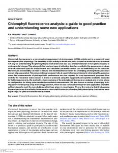
shall show later, our analyses indicate that even a fairly crude estimate of atmospheric effects is sufficient. The dominant source of uncertainty in fluorescence-based measurements is in the physiological processes of the phytoplankton themselves (Letelier and Abbott, 1996). Chlorophyll fluorescence will increase the amount of water-leaving radiance at 683 nm (Gordon 1979; Topliss 1985; Topliss and Platt 1986) than would be expected for chlorophyll-free water. The amount of this increase will depend on several factors including the specific absorption of chlorophyll, fluorescence quantum efficiency, the amount of incident sunlight, and various atmospheric effects. However, judicious choice of wavelengths should tend to minimize the effects of the atmosphere. Thus the main component of the algorithm is the estimation of the increased radiance caused by fluorescence. By defining a baseline underneath the expected fluorescence peak, one can estimate the relative contribution to the upwelled radiance field by chlorophyll fluorescence. This baseline will be linear, based on MODIS channels places on either side of the fluorescence peak. FLH will then simply be the intensity of upwelled radiance in MODIS band 14 (676.7 nm) above the baseline created from bands 13 (665.1 nm) and 15 (746.3 nm). The figure below shows a schematic of the FLH algorithm.

MODIS normalized filter spectra of bands #13, 14 and 15 and Ocean Surface Exitance for 0.01 and 10 mg Chl/m3 1

1.40E-01 10 mg/m3 (1st axis)

0.9

0.01 mg (right axis) 0.8

1.00E-01

0.7

L 14

10 mg (left axis)

0.6 8.00E-02 0.5

L13

FLH

Exitance, W m -2 µm -1 Exitance (W/m2/um)

1.20E-01

0.01 mg/m3 (2d axis)

6.00E-02

L baseline

0.4

0.3

4.00E-02

10 mg Chl /m3 bas elin e

0.2

Normalized Transmitance and Ocean Surface Exitance (W/m2/um)

#13 (2d axis) #14 (2d axis) #15 (2d axis)

2.00E-02

0.1

L15 0 650

λ13

675

λ14

700

725

750

λ15

Wavelength (nm)

0.00E+00 775

Wavelength, nm

Figure 1. A schematic of the FLH algorithm, with dash/dot lines representing the normalized transmittance of MODIS bands 13, 14, and 15. The solid lines show the spectral distribution of upwelling radiance above the surface of the ocean for chlorophyll concentrations of 0.01 and 10 mg/m3. The fluorescence per unit chlorophyll is assumed to be 0.05 W/m2/µm/sr per mg chlorophyll. Chlorophyll fluorescence efficiency refers to the conversion of incident sunlight into chlorophyll fluorescence. CFE requires an estimate of the amount of incoming solar radiation that is absorbed by phytoplankton in the near-surface waters since the 7

fluorescence signal measured by MODIS will originate here. This estimate will be provided by MOD22 and is based on estimates of chlorophyll concentration, instantaneous photosynthetically available radiation, and the specific absorption of chlorophyll. Details can be found in the ATBD by Carder. The ARP product will be converted into radiance units as the original product will be expressed in terms of photons absorbed. Because the fluorescence peak can sometimes be below the baseline, we will add a constant radiance to all of the FLH values. This constant (0.05 W/m2/µm/sr) corresponds to the minimum amount of fluorescence expected based on historical measurements. This modified FLH will then be normalized by the converted ARP to estimate CFE. For both the FLH and CFE products, the input data sets will be level 2 data. For areas of chlorophyll greater than 1.5 mg/m3, we will calculate FLH and CFE on a per pixel basis. For areas with chlorophyll less than 1.5 mg/m3, we will examine 5 by 5 pixel regions to improve SNR in regions where the fluorescence signal will be small. We will average the appropriate input products (normalized water-leaving radiances, ARP) to decrease the noise level. We assume that noise will decrease as roughly 1/ n , where n is the number of clear pixels. 3.1.2.

Mathematical Description

The mathematics of both the FLH and the CFE algorithms are straightforward. After correcting for scan geometry, calibration, illumination, and the atmosphere, we take the normalized upwelled radiances as follows: FLH = L14 −

FG L Hλ

g IJK

− L15 * λ14 − λ13 + L13 13 − λ15

b

13

(1)

where the subscript refers to the MODIS band number. The formalism of (1) establishes a baseline between bands 13 and 15 and measure the peak height (band 14) above this baseline. A graphical representation of the algorithm is shown below: C

A

x B

D y E

F

In this representation, LA is the short wavelength band, LF is the long wavelength band, and LC is the center or fluorescence wavelength. The distance between points B and E is denoted as x and the distance between point E and F is denoted as y. Using a simple like-triangles calculation, we may calculate FLH as: 8

FLH = CD = LC − ( LF + DE )

(2)

This can be simplified as:

FLH = LC − ( LF + (( LA − LF ) * y / ( x + y )))

(3)

In this case, we have simply rearranged (2) and expressed FLH as a linear function of the two baseline wavelengths and the fluorescence band. Other researchers have suggested using a curvilinear baseline, but our analysis (Sec. 3.2) suggests that this not warranted. We also note that a band closer to 700nm, rather than 750 nm, would have improved the FLH response. The GLI sensor has such a band. CFE will be estimated by adding a constant radiance (FLHmin) to the FLH value and then normalizing by the radiance absorbed by phytoplankton in the upper ocean (ARPradiance). FLH + FLHmin CFE = (4) ARPradiance These algorithms have been embedded in the MODIS Oceans Team products processing system developed at the University of Miami. 3.2

Performance and Uncertainty Estimates

A complete sensitivity analysis of the FLH algorithm was published in Remote Sensing of the Environment (Letelier and Abbott, 1996). We present a summary of this paper here. As CFE is largely dependent on FLH, we expect that uncertainty in CFE will follow uncertainty in FLH. There are three processes that will affect measurements of FLH. The first will be changes in the absorption and scattering properties of the atmosphere. Scattering will dominate at shorter wavelengths, but the presence of specific absorption features can be important in the fluorescence wavelengths. In particular, the oxygen absorption bands at 687 and 760 nm and the water vapor band at 730 nm will significantly influence the shape of the fluorescence peak such that it deviates from a pure Gaussian curve. By designing MODIS such that these absorption features are avoided, these problems are generally reduced. The second process involves the performance of the MODIS instrument itself. This is the only component that we can control (at least before launch). The final process is physiological change in the phytoplankton which will result in variability in FLH. As discussed earlier, this can be troublesome if we try to estimate chlorophyll concentrations from FLH as the amount of fluorescence per unit chlorophyll is not constant. The amount of fluorescence will vary as a function of the amount of light absorbed as well as the quantum efficiency of fluorescence. These quantities can vary according to the species and physiological state of the algae. Specifications of the filter spectrum and signal to noise ratio (SNR) for each band are presented in Table 1. Based on Eq. 1 and assuming that noise is independent between bands, the SNR of the baseline may be calculated as

9

 1 1 1 1  = +  −  * ( λ15 − λ14 )/ ( λ15 − λ13 ) SNRbaseline SNR15  SNR13 SNR15 

The SNR of the FLH is calculated as: 1 1 1 = + SNRFLH SNR14 SNRbaseline

(5)

(6)

Given the specifications of Table 1, the SNR of FLH is 752. MODIS Band #

Center Wavelength Tolerance

Bandwidth Tolerance

up

down

(nm)

(nm)

(nm)

13

665.1

1

14

676.7

15

746.3

Band SNR

upper

lower

(nm)

(nm)

(nm)

2

10.3

4.2

6.1

1368

1

1

11.4

5.8

5.4

1683

2

2

10

5.1

5.3

1290

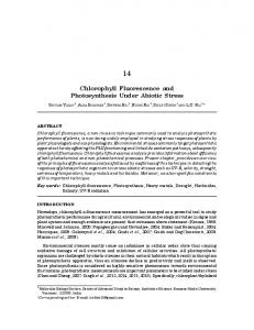
Table 1. Specifications for the fluorescence-related bands on MODIS (W. Barnes, pers. comm.) A realistic range of upwelling radiance at the top of the atmosphere (TOA) for λ = 685 nm and a solar zenith angle of 50.7° is 8-20 W m-2 sr-1 µm-1 (Fischer and Schlüssel 1990). The lower end of this range corresponds to an atmospheric turbidity factor of 0.5 (visibility = 88 km), and the upper value corresponds to a turbidity factor of 10 (visibility = 6 km). A similar value is obtained when the radiance spectrum at the TOA is calculated using a marine atmosphere model with a visibility of 50 km, a solar zenith angle of 60°, and the ocean spectrum without chlorophyll as input datasets for LOWTRAN 4.2 (Kneizys et al., 1988). The upwelling radiance at the TOA for λ = 685 nm obtained through this method is 8.65 W m-2 sr-1 µm-1. However, given the characteristics of MODIS band 14, a more accurate estimate of the sensitivity is obtained by using the calculated TOA upwelling radiance at λ = 676.7 nm. In this case, the upwelling radiance at TOA calculated using LOWTRAN is 9.05 W m-2 sr-1 µm-1. The TOA spectra are shown in the figure below.

10

12

1.20E-01

10 mg

1.00E-01

8

8.00E-02

0.01 mg 6

6.00E-02

4

4.00E-02

2

2.00E-02

0 650

670

690

710

730

750

Normalized band transmitance

Radiance, W m -2 µm -1 sr-1

10

0.00E+00 770

Wavelength, nm

Figure 2. Baseline correction for the FLH algorithm for chlorophyll values of 0.01 and 10 mg/m3 for spectra at the top of the atmosphere. The minimum signal of detection (MSD) based on the SNRFLH and the TOA radiance at λ = 676.7 nm is :

MSD =

RadianceTOA 9.05Wm − 2 sr − 1 µm − 1 = = 0.012Wm − 2 sr − 1µm − 1 SNRFLH 752

(7)

However, this MSD is calculated for an atmosphere with low turbidity. Under high turbidity, the MSD increases to 0.026 W m-2 sr-1 µm-1 and the sensitivity of the FLH algorithm decreases. To convert MSD into chlorophyll, we must account for atmospheric attenuation, transmission through the air/sea interface, interference by suspended particulates, and variability in the fluorescence:chlorophyll ratio. For a typical mid-latitude oceanic atmosphere, the radiative transfer of the sea surface fluorescence signal measured at λ = 676.7 nm to the TOA is close to 80%. Increasing the ocean atmospheric aerosol content from a turbidity factor of 0.5 (visibility = 90 km) to a factor of 10 (visibility = 6 km) decreases the absolute atmospheric transfer of the fluorescence signal by less than 30%. Variations in the atmospheric water vapor content also affect the recovery of the TOA fluorescence signal by less than 20%. These results are consistent with the results of the analyses performed by Fischer and Schlüssel (1990). We believe that 30% is a conservative estimate of the loss of the fluorescence signal through the atmosphere. Hence, 0.017 W m-2 sr-1 µm-1 at λ = 676.7 nm is the minimum fluorescence signal at the ocean surface detectable at the TOA by the MODIS FLH algorithm.

11

Two processes contribute to a decrease of the upwelling radiance when the light crosses the sea-air interface. The principal process is refraction of light. The loss due to this process is approximately 45%. The second process is reflection. The loss in signal is small for angles of 0-40° to the vertical under calm conditions (2-6%) but can increase to 16-27% for the angles in the upper side of this range when the sea-surface becomes rough (Kirk 1994). By combining both processes, Austin (1980) proposes a correction factor of 0.544 to extrapolate the upwelling radiance at the sea surface to the upwelling radiance just below the surface. If this correction factor is incorporated in the calculated minimum fluorescence signal measurable at the sea surface, the resulting minimum fluorescence signal in the upper water column required to be detectable by MODIS is 0.032 W m-2 sr-1 µm-1 at λ = 676.7 nm. The conversion of this signal into chlorophyll values will depend on the fraction of energy absorbed by chlorophyll that is released in the form of fluorescence. This fraction is known as the chlorophyll fluorescence quantum yield (Φ f):

FLH = Φ f * Ia

(8)

where Ia is the light flux absorbed by the photosystem. Because most chlorophyll fluorescence originates in PS II, Ia may be approximated by:

Ia = Io * σ II * nII

(9)

where Io in the mean incident irradiance, σII is the mean optical absorption of PS II, and nII is the concentration of PS II, having a “typical”value of one unit per 500 chlorophyll a molecules (Kolber and Falkowski, 1993). However, under saturated light conditions Ia becomes independent from Io . If we assume σII to be constant under light saturated conditions, the light flux absorbed per unit chlorophyll is nearly constant and the FLH per unit chlorophyll a is proportional to Φ f as follows:

FLH I = Φ f * a = cte.*Φ Chl. a Chl. a

(10)

f

Published values of Φ f vary between 0.0015 and 0.1 with a mean of 0.0035 (Günter et al. 1986, cited in Fischer and Kronfeld 1990). However, based on field measurements, a range from 0.002 to 0.02 appears to cover most cases in marine environments (Gordon 1979). Fischer and Kronfeld (1990), assuming Φ f = 0.003, calculated a conversion factor of 0.05 W m-2 sr-1 µm-1 per mg chlorophyll at λ = 685 nm for light saturated photosynthetic conditions. A conversion factor of 0.057 W m-2 sr-1 µm-1 per mg chlorophyll at λ = 676.7 nm is found when reconstructing the chlorophyll fluorescence spectrum from the ocean surface spectra given by W. Barnes (pers. comm.). Using this conversion factor and the calculated detection limit of the fluorescence signal in the upper water column, based on the specified SNR, and the sea surface and atmosphere transmission, the limit of detection of changes in chlorophyll concentration is approximately 0.5 mg m-3 (Fig. 3). This limit of detection decreases to 1.3 mg m-3 under turbid atmospheric conditions.

12

3500

3000

Baseline : FLH

2500

2000

1500

1000

500

0 0

1

2

3

4

5

6

7

8

9

10

Chl a, mg m -3

Figure 3. Detection limit of the FLH algorithm on a clear day (visibility = 90 km) as a function of the fluorescence to chlorophyll conversion factor (u = 0.01, s = 0.03, l = 0.05, n = 0.08 W m-2 µm-1 sr-1). Values below the dashed line are detectable. While atmospheric turbidity may strongly affect the limit of detection of the FLH algorithm by increasing the TOA radiance, the principal source of error in the interpretation of changes in the fluorescence signal arises from neglecting the role that algal physiology has in the production of fluorescence. The fluorescence quantum yield (Φ f) may vary an order of magnitude in marine environments as a result of changes in phytoplankton species composition, nutrient availability, temperature and light. The FLH signal per unit chlorophyll is proportional to Φ f under light-saturated conditions, the detection limit of the FLH algorithm cannot be defined in terms of chlorophyll unless Φ f is known. The limit of detection under clear sky conditions may vary from less than 0.3 to greater than 2 mg m-3 when varying the fluorescence to chlorophyll conversion factor from 0.08 to 0.01W m-2 sr-1 µm-1 per mg chlorophyll (Fig. 3). Furthermore, observed spatial and temporal variations in the FLH signal do not necessarily reflect changes in chlorophyll concentration unless Φ f is kept constant. Understanding the variability of the chlorophyll natural fluorescence due to changes in phytoplankton physiology is a critical step in the interpretation of changes observed in the FLH. Other parameters that will affect the magnitude of the FLH signal are the size of particles and their effect on scattering, the concentration of suspended matter not containing chlorophyll, and the concentration of yellow substance (Gelbstoff). However, based on the results presented by Fischer and Kronfeld (1990), we have assumed that none of these parameters will modify the FLH by more than 30%. These effects are small compared with the potential variability introduced by changes in the atmosphere turbidity and chlorophyll fluorescence efficiency.

13

If noise is independent between pixels the SNR of individual bands increases fivefold when analyzing a 5 by 5 pixel signal. Hence, in areas of the ocean where surface water characteristics are homogeneous over scales larger than 5 by 5 pixels (nominally 25 km2 at nadir), the limit of detection of chlorophyll concentrations for clear atmospheric conditions, assuming a conversion factor of 0.05 W m-2 sr-1 µm-1 per mg chlorophyll, decreases to 0.10 mg m-3. 3.3

Algorithm Evolution

The first place for changes in the structure of the algorithm is in the area of atmospheric correction. However, the correction would essentially follow the same form as that for the other water-leaving radiances, as described by Gordon. To evaluate the performance a more sophisticated atmospheric correction, we would calculate FLH with both correction schemes and examine the data for systematic errors. Regions of persistent low humidity (such as at high latitudes) and high humidity (such as the tropics) will be candidate study areas as well as areas subject to rapid changes in air mass types, such as western boundary current regions. Time series of these areas will be examined for both systematic biases in the FLH estimates as well as for rapid shifts in FLH that might be indicative of changes in humidity. However, our error analysis (Letelier and Abbott 1996) suggests that even crude atmospheric corrections are a small part of the FLH error. The most important component of FLH error is the fluorescence quantum efficiency. The other potential area for evolution is the use of multiple data sources to estimate FLH. Besides Terra and PM-1, MERIS and eventually GLI will also measure sunstimulated fluorescence. Although the calculation of FLH for each sensor will be essentially unchanged, blending of the data sets will require considerable research. Issues such as binning, which sensor to select in cases of multiple observations, crosscalibration, etc. will need to be addressed. The different crossing times for the various sensors that are capable of chlorophyll fluorescence measurements may allow us to refine our productivity models by examining daily variations in fluorescence quantum yield. 3.4

Basis for Estimates of Primary Productivity using FLH and CFE

Our primary focus for algorithm evolution is to utilize variability in fluorescence quantum efficiency to improve our estimates of primary productivity. FLH is a measure of the absolute amount of energy released by phytoplankton in the form of fluorescence. This value is a function of the radiation absorbed by phytoplankton and the probability for a given absorbed photon to be re-emitted as fluorescence. This probability, known as the quantum yield of fluorescence (Φ f) provides information with regard to the energy distribution in the photochemical apparatus (Krause and Weis 1991). To estimate the fluorescence quantum yield we plan on using the FLH product as well as the Absorbed Radiation by Phytoplankton (ARP) provided by Carder. Dividing FLH by ARP will allow us to estimate of the amount of energy absorbed by phytoplankton that is re-emitted as fluorescence, also termed chlorophyll fluorescence efficiency (CFE)

14

However, to derive photoautotrophic carbon fixation from APR and CFE we need to understand the relation between the fraction of energy used for carbon fixation (Φ C) and the fraction released as fluorescence (Φ f). Butler’s tripartite model of the photosystem (Butler 1978) suggests that there is an inverse relationship between Φ f and Φ C However, this relationship is affected by environmental factors such as light saturation, nutrient limitation, and temperature. 3.4.1 Field Studies Our studies of FLH as a predictor of phytoplankton photoadaptive state is motivated by field observations of fluorescence made from quasi-Lagrangian drifting buoys that were equipped with spectroradiometers. These sensors measure upwelled radiance at the SeaWiFS wavelengths as well as at 683 nm. Letelier et al. (1997) discuss results from a drifter deployment in the Southern Ocean. In this example, a drifter was deployed in the Drake Passage area in austral summer 1994-1995. The drifter included a spectroradiometer that measured upwelling radiance at the SeaWiFS wavelengths as well as at 683 nm. A drogue was attached below the surface float so that the drifter would follow ocean currents at 15 m depth. We estimated chlorophyll using the radiance ratios developed by Clark (1981), analogous to the MODIS standard data product for chlorophyll. Fluorescence at 683 nm was corrected for backscatter using the 670 nm band; this is similar to the FLH approach for MODIS. Downwelling irradiance incident at the sea surface was measured using a single band (490 nm) irradiance sensor mounted on the top of the surface float. Together, the changes in amount of fluorescence per unit chlorophyll per unit sunlight are proportional to changes in Φ f. Letelier et al. (1997) defined an apparent fluorescence quantum yield as the slope of the regression of fluorescence per unit chlorophyll and downwelling irradiance at 490 nm. This slope was based on 48-hour averages, thus eliminating the effects of diurnal photoadaptive processes. This particular bio-optical drifter was trapped in a cyclonic eddy for over forty days. During this period, Letelier et al. (1997) calculated vertical velocity based on the conservation of potential vorticity and the measured horizontal velocities associated with the drifter displacement. Regular, short-term variations in the apparent fluorescence quantum yield were observed as well as in the relative depth of the eddy’s upper layer. The correlation between layer thickness and fluorescence quantum yield are probably driven by changes in nutrient availability. Decreases in layer thickness correspond to upward vertical velocities. Rough estimates of the vertical velocity are on the order of 20-60 m/day. Given that iron is probably the limiting micronutrient in this region, we suggest that iron stress may be alleviated during these upwelling events, thus reducing the fluorescence quantum yield and increasing photosynthetic quantum yield. During downwelling, the situation is reversed.

15

SST, °C

4 3 2

chl, mg m -3

1

A

0 0.6 0.4 0.2

B Fluor. slope

0.0 0.003 0.002 0.001

C

h ho-1

0.0 1.00 0.75 0.50 0.25

D

0.00 0

10

20

30

40

50

60

Days since 01/01/95

Figure 4. Temporal variability of (A) sea surface temperature, (B) chlorophyll concentration, (C) Apparent Φ f,, and (D) relative depth of the upper layer of the water column sampled by the drifter within the cyclonic eddy. Dotted lines in (C) show the 95% confidence interval. In regards to MODIS, it is interesting to note that the averaged estimates of fluorescence quantum yield seemed to fall into two categories, depending on the nutrient regime. As MODIS will observe the ocean only under conditions of full sunlight, we will not be able to conduct an analysis similar to the one used for the drifter data. However, if the fluorescence quantum yield falls only into a few, easily distinguishable categories, then we should be able to measure CFE with MODIS over a period of several days to estimate primary productivity. That is, the variability in CFE will give an indication of the photoadaptive state of the phytoplankton, information that in turn can be used to estimate the quantum yield of photosynthesis. We will be conducting both field and laboratory experiments to develop such a model. In the California Current, we (Abbott and Letelier, 1998) interpreted observed short fluorescence/chlorophyll time scales as suggesting that phytoplankton light harvesting (as represented by chlorophyll content) and light utilization (as represented by fluorescence) are not in balance, at least on the time scale of days. Fluorescence per unit chlorophyll may change rapidly so that although phytoplankton are harvesting light, they were not be able to utilize this light in photosynthesis and re-emitted some of it as

16

fluorescence (Kiefer and Reynolds, 1992). We assume that the number of active reaction centers is changing rapidly relative to the amount of light-harvesting chlorophyll on a time scale of days. In this situation, the ability of phytoplankton to utilize the constant amount of harvested light changes rapidly, leading to short time scales for fluorescence/chlorophyll. On the other hand, if the amount of harvested light changes rapidly relative to the ability to utilize light, then fluorescence should change in parallel with the amount of light-harvesting chlorophyll. Rapidly-changing values of chlorophyll lead to rapid changes in the amount of harvested light but there are no parallel changes in the ability to process this light in the reaction centers. This leads to short decorrelation scales for chlorophyll whereas fluorescence/chlorophyll are temporally stable with long decorrelation scales. Thus in one case, the fluorescence/chlorophyll decorrelation scale are longer than the chlorophyll scale and in the other the fluorescence/chlorophyll scale are shorter. An imbalance between light harvesting and light utilization results in different decorrelation scales for chlorophyll and fluorescence/chlorophyll. We cannot say definitively whether the time scale for chlorophyll would be larger or smaller than the fluorescence/chlorophyll scale. In the case where the fluorescence/chlorophyll time scale is shorter than the chlorophyll time scale (light utilization changes faster than light harvesting), nutrient limitation (and the response to variability in the amount of available nutrients) changes the number of reaction centers. In contrast, light limitation leads to changes in the amount of chlorophyll relative to the number of reaction centers, resulting in long fluorescence/chlorophyll time scales relative to the chlorophyll time scales (light harvesting changes faster than light utilization). Similar arguments were proposed by Letelier et al. (1997) to explain observed changes in apparent fluorescence quantum yield in an ocean eddy. Our observations in the nearshore region of the California Current suggest that the fluorescence/chlorophyll time scale is smaller than the chlorophyll time scale, implying that nutrient availability may be the critical process in this region. This interpretation should be tempered with the sometimes contradictory evidence from laboratory experiments. As shown by Cullen and Lewis (1988), fluorescence and photosynthesis are linked through a complex set of reactions, each with its own time scale which depends in part on species composition and the degree of environmental perturbation. Babin et al. (1996) assumed a steady-state (in contrast to the transient responses which dominate the California Current) to examine the influence of environmental variability on sun-stimulated fluorescence. Although they noted that a decrease in nutrients would decrease the proportion of functional reaction centers, Babin et al. (1996) did not attempt to predict the quantum yield of fluorescence in this case. However, Greene et al. (1992) did present evidence for an increase in fluorescence yield following the transfer of phytoplankton cultures to nitrogen or ironpoor media, although at lower irradiance values. Chlorophyll fluorescence varies on a wide range of time scales and is sensitive to changes in nutrient stress and species composition (Falkowski and Kolber, 1995). Although this change in the quantum yield of fluorescence greatly complicates the use 17

of fluorescence to estimate phytoplankton biomass, this variability may be used to bridge the gap between the small scales associated with physiological adaptations and the longer scales associated with ecosystem function (Falkowski and Kolber, 1995). In regions of strong vertical motion (such as in areas of active upwelling in the nearshore region of the California Current), fluorescence per unit chlorophyll will change rapidly. Our results have implications for primary productivity models that are based on remote sensing observations. Behrenfeld and Falkowski (1997) demonstrate that the performance of productivity models depends strongly on optimal assimilation efficiency (a measure of photoadaptation). If fluorescence quantum yield is an indicator of photoadaptation (Falkowski and Kolber, 1995), then our results suggest that there may be different strategies of photoadaptation as phytoplankton communities shift from non-equilibrium to equilibrium. In other words, phytoplankton may always be “tracking”an optimal photosynthetic efficiency, but the closeness of this tracking may vary significantly. Our results support the conclusion of Behrenfeld and Falkowski (1997) that more effort must be placed on understanding the linkages between phytoplankton physiology and environmental variability. 3.4.2 Laboratory Studies To understand how nutrients and light affect the distribution of energy in the photosystem, we are studying under controlled conditions the response of the photosystem to changes in light quality as well as to changes in nitrogen, phosphorus, and iron supply. Continuous cultures of different phytoplankton taxa are being grown in our laboratories. We are using a Fast Repetition Rate (FRR) fluorometer to make continuous measurements of photosynthetic parameters such as the effective cross section of photosystem II and maximum change in quantum yield of fluorescence. Combining these measurements with measurements of solar induced (natural) fluorescence will help us to accurately interpret changes Φ f and how they relate to changes in Φ C. This is a critical piece of information required to develop a mechanistic model of primary production that uses phytoplankton natural fluorescence.

18

200

PAR, µmol quanta m-2 s-1

150 100 50 0 212

212.1 212.2 212.3 212.4 212.5 212.6 212.7 212.8 212.9

213

-4

11

Fluorescence yield, Volts

x 10

10

9

8 212

212.1 212.2 212.3 212.4 212.5 212.6 212.7 212.8 212.9

213

Figure 5. A sample run of the chemostat, showing PAR and fluorescence yield during a diel cycle. Figure 5 shows a one-day cycle of PAR and fluorescence yield from the chemostat. We have added a computer control to the light source in order to provide a more realistic day light environment. The small peaks at the beginning and end of the daylight cycle are artifacts of the initial warm-up and turndown of the light source. Note the increase in fluorescence yield at the beginning and end of the “day,”part of the photoadaptive process. The mid-day depression is still under study, but it is probably related to photoadaptation of the reaction centers.

19

Maximum fluorescence yield -4

11.5

x 10

Fluorescence yield, volts

11 10.5 10

5 AM Fluoresc. yield

9.5 9 8.5 8 7.5 7 210

Noon Fluoresc. yield 211

212

213

214

215

216

217

218

Time, day of year

These patterns are reproducible over many days and weeks, as shown in Figure 6. There are changes in the pattern, which we think are related to changes in the nutrient environment of the chemostat. Figure 7 shows a summary of the descriptive statistics shown in Figure 6.

x 10-3 0.18

1.4

5 AM fluoresc. yield

1.2

Maximum fluorescence yield

0.14

1 0.12 0.8

0.1 0.08

0.6

Maximum diel fluorescence

0.06

0.4

Noon fluoresc. yield

0.04

Fluorescence yield, Volts

0.16

Maximum diel fluorescence, Volts

F l u o r

Figure 6. A one-week record of fluorescence yield from the chemostat.

0.2

0.02 0

0 200

205

210

215

220

225

Time, day of year

Figure 7. Time series of the descriptive statistics shown in Figure 6.

20

Fluorescence efficiency (initial fluorescence/PAR slope)

Saturating PAR 45 0.005 40

35

Fluorescence efficiency

0.0045

30

0.004

25

20 0.0035 15

10

0.003 210

215

220

225

Saturating PAR, µmol quanta m -2 s-1 (PAR at initial deviation from linearity)

50

0.0055

230

Time, day of year

Figure 8. Time series of fluorescence efficiency and saturating photosyntheticallyavailable radiation (PAR). We used the information in Figure 7 to derive an estimate “fluorescence efficiency” which was based on the initial slope of fluorescence versus PAR at low light levels at the beginning of the “day.” We also estimated “saturating PAR”which we defined as the point where the fluorescence yield began to deviate from a linear function of PAR (see Figure 7). In the specific data set shown in Figure 8, we can see how the phytoplankton culture adapt to a new nutrient regime. The main objective during the first phase of our research is to evaluate the range of scales of variability that can be studied by monitoring phytoplankton sun stimulated fluorescence. The results from these studies will help in our interpretation of the scales of variability in phytoplankton fluorescence yield observed in pelagic environments. Two major questions to be addressed during with the chemostat are: • What are the time-lag response of fluorescence to changes in nutrient (nitrogen, phosphorus, and iron), light, and temperature regimes? • Is there a correspondence between the magnitude of the fluorescence response and the magnitude or type of environmental change? 3.5

Programming and Procedural Considerations

The FLH algorithm is simple, as it is merely a manipulation of normalized, calibrated radiances from the Miami-developed ocean processing system. The bulk of the computation will take place in this system. After application of the FLH algorithm, the data will then be available for remapping into standard grids. The registration process 21

will be part of the Miami system. CPU load should be relatively small; therefore the use of lookup tables (as opposed to direct calculation) will not be efficient. CFE is a simple combination of FLH and ARP. C code for both FLH and CFE has been delivered to Miami and integrated into the MODIS oceans processing. A 5 by 5 array will be centered on each pixel. The algorithm will first check the corresponding chlorophyll from the Case 1 chlorophyll product calculated using Clark’s algorithm (MOD19). If chlorophyll is less than 1.5 mg/m3, then the radiances from the 5 by 5 bin will be averaged; this average will be used in the FLH and CFE calculations. The coefficient of variation will also be calculated. The 5 by 5 array will then be moved over one pixel, and the process will be repeated. At the end of the scan line, the array will be shifted up one line. Thus, the output product will consist of FLH and CFE calculated at every pixel, and the number of pixels used to calculate FLH may range from 1 to 25. 3.6

Calibration and Validation

Validation will rely on a three-part approach. The first approach will rely on systematic studies of large volumes of MODIS observations over several seasons to quantify spatial and temporal error patterns. The second component of our validation studies is an extension of this approach and relies on statistical comparisons of MODIS observations with similar measurements from MERIS and GLI. The third approach will be comprehensive in situ studies, conducted at a few representative sites in the world ocean that span a spectrum of oceanic and atmospheric conditions. The basic FLH algorithm is a simple estimate of peak height. The more critical factor will be the assessment of instrument and atmospheric effects on the basic input data sets. The first stage in validation will be to compare the FLH results with other MODIS data products. For example, FLH should be similar to the patterns of chlorophyll; are there systematic differences? How does FLH compare with estimates of aerosol radiance? The next stage will be to compare FLH with geographic and geophysical properties. For example, are there systematic changes in FLH across a scan line, indicating a dependence on satellite look angle and hence path radiance? Does FLH change near the edges of clouds, where aerosol concentrations may be higher? Are there systematic seasonal changes? Other data sets such as wind velocities (from scatterometers) will be used in for validation. Our plan is to use large volumes of MODIS data products to seek out such systematic relationships. The second approach to validation will be to compare MODIS estimates of FLH with other satellite-based estimates of FLH. Both MERIS and GLI will make measurements in the fluorescence region, although it is likely that the exact bands will differ slightly from MODIS. Thus such comparisons will not be based on exact comparison of FLH estimates from the same pixel location, but rather on general trends and patterns. For example, for regions that are simultaneously observed by MODIS and either MERIS or GLI will be analyzed for trends and biases. (In this case, “simultaneous”means within a few hours.) Such comparisons will allow us to examine estimates of FLH under

22

different viewing conditions to characterize the effects of path radiance. These studies will be conducted in different geographic locations and in different seasons. The final component of our validation plan relies on a set of focused in situ observations. The framework for field validation studies will be based on the framework developed for SIMBIOS. Our activities will build on the foundation established for SIMBIOS in terms of protocols and data management. The basic water-leaving radiances for the FLH algorithm will be validated in a manner similar to the other ocean color bands as described by Gordon. Because of the intense variability in the ocean on mesoscales along with lower frequency processes such as the El Niño/Southern Oscillation (ENSO) events, it is not possible to sample all of the critical conditions and regions adequately. Instead, intensive campaigns will be carried out a few sites that span a wide range of oceanographic and atmospheric conditions. To assess the effects of lower frequency variability, autonomous samplers will be deployed in a few locations for several years. These stations will be much less sophisticated than the bio-optical mooring developed for the SeaWiFS and MODIS by Clark. By keeping costs low, more sensors will be deployed as either fixed moorings or free-floating drifters in order to characterize temporal and spatial variability. The long-term goal of this approach is to develop a body of knowledge of the error fields of the data sets that can be used in data assimilation models. Before the launch of EOS, we conducted extensive field measurements at two locations: the Joint Global Ocean Flux Study (JGOFS) site at the Hawaii Ocean Time-series (HOT) north of the island of Oahu and at the Polar Front as part of the JGOFS Southern Ocean study. The HOT effort is a biogeochemical mooring that is deployed at 157°50’W, 23°N in conjunction with Station ALOHA which is located about 20 km away. The mooring (known as HALE ALOHA) supports meteorological, bio-optical, chemical, and physical measurements in the upper 300 m of the ocean. An automated water sampler is also be attached to the mooring. This site complements the MOBY site which is located west of the island of Lanai and is focused more heavily on precise bio-optical measurements in support of SeaWiFS and MODIS calibration activities. Our contribution to the mooring are Satlantic irradiance sensors which measure irradiance at the MODIS oceans wavelengths. The bio-optical measurements are analyzed in conjunction with the more extensive suite of biological and chemical measurements to develop and validate productivity algorithms as well as assess processes that affect both FLH and CFE. We will also use our Fast Repetition Rate (FRR) fluorometer in this assessment. The second field site is part of the final U.S. JGOFS process study in the Southern Ocean known as Antarctic Environment Southern Ocean Process Study (AESOPS). We deployed 12 bio-optical moorings in the Polar Front at 170°W, 65°S, relying primarily on funding from the National Science Foundation. This array was established in October 1997 and was in the water for five months. The moorings consisted of expendable current meters and Satlantic irradiance sensors. Bio-optical drifters were also deployed during the 1997-1998 mooring experiment. (Three bio-optical drifters were deployed in the Polar Front in September 1996 using MODIS funding.) Ship-based observations 23

were also made of near-surface upwelled radiances, pigments, fluorescence, and primary productivity. A manuscript has been submitted (Abbott et al., submitted). Figure 9 shows the mooring-derived chlorophyll time series. The general pattern is similar between moorings: a pronounced spring bloom began in early December 1997, peaked in late December and then began to decay over the next month. We calculated sun-stimulated fluorescence per unit chlorophyll (F/C) to estimate the photoadaptive state of the phytoplankton community during this bloom event. Chlorophyll (All Moorings) 3.5

3.0

3

Chlorophyll (mg/m )

2.5

2.0

1.5

1.0

0.5

0.0 300

350

400

450

Mooring 2 Mooring 4 Mooring 5 Mooring 6 Mooring 7 Mooring 8 Mooring 9 Mooring 10 Mooring 12

Day

Figure 9. Time series of chlorophyll from the bio-optical moorings in the APFZ, 19971998. Figure 10 shows the time series of F/C. As with the chlorophyll time series, there is a generally repeatable pattern at each mooring, but there was more variability. There is an increase in F/C just before the increase in chlorophyll. F/C then drops to a very low value. It remained low, even as chlorophyll concentrations began to decline. About one month after the peak in chlorophyll concentration, F/C began to increase at most of the moorings, especially moorings 4 and 7.

24

Fluorescence/Chlorophyll (All Moorings)

3

Fluorescence/Chlorophyll (uW/cm /nm)/(mg/m )

2.0

2

1.5

1.0

0.5

0.0 300

350

400

450

Mooring 2 Mooring 4 Mooring 5 Mooring 6 Mooring 7 Mooring 8 Mooring 9 Mooring 10 Mooring 12

Day

Figure 10. Time series of F/C from the bio-optical moorings, 1997-1998. We interpret these results as follows. The initial bloom in chlorophyll is initiated by the sudden increase in stratification of the upper ocean in early December. This inhibits deep mixing, allowing phytoplankton to spend more time in the well-lit upper waters. The sudden change in the light environment also increase F/C, as phytoplankton are not photoadapted to this new regime. As the phytoplankton adapt, F/C drops rapidly, indicating high productivity. However, chlorophyll concentrations begin to decrease before F/C increases, suggesting that the light utilization properties of the phytoplankton were not under stress. Instead, phytoplankton were probably limited by a nutrient not involved in phytoplankton photosynthesis. As spring blooms in the Antarctic Polar Frontal Zone are generally dominated by diatoms, depletion of silicate is a likely cause for the collapse of the spring bloom. Silicate is not involved in phytoplankton energetics, unlike other nutrients. Eventually, F/C begins to increase, implying that the phytoplankton community began to be limited by a nutrient involved in photosynthesis. Since nitrate is always abundant in the APFZ, it is likely that the increase in F/C is related to iron limitation. Note that F/C increases the most in late summer, when stratification is the strongest. The approach begun in the pre-launch phase will continue after the launch of EOS Terra in 1999. The HALE ALOHA mooring work will continue at least until 2000. However, the Southern Ocean JGOFS program will have concluded, and we hope to continue Southern Ocean work in collaboration with Dr. John Parslow (CSIRO Australia). The study site will be at the Polar Front but farther west at 145°E. Measurements (moorings and drifters) similar to the JGOFS project will be conducted, but the density

25

of sampling will be less. The focus of this experiment will be to estimate seasonal and interannual variability of the model parameters. We will participate in the two MOCEAN experiments planned soon after the launch of Terra. The first will focus on the eastern Pacific between San Diego and Acapulco, and is tentatively scheduled for October 1999. This cruise will transit several types of water masses for initial validation of the MOCEAN algorithms. The second experiment is planned for the upwelling system off Northwest Africa in 2000. This experiment is focused more on the effects of atmospheric processes on the MODIS retrievals, especially in the presence of intense loading of dust from the Sahara. This region will provide a valuable comparison with the high latitude site at the Polar Front and the low latitude site off Hawaii where dust loading is much smaller. The last target area will be the productive waters off Oregon which are dominated by coastal upwelling. This mid-latitude site is easily accessible by small boat from the Oregon State University marine facility at Newport, Oregon. We plan to collect regular monthly samples of bio-optical and standard biological variables during the first years of Terra. We have collected several preliminary data sets using the FRR and the TSRB. We participated in a cruise in the coastal upwelling region off Oregon in September 1998. We deployed the new FRR fluorometer and the Satlantic TSRB-II. The FRR worked quite well this time, although there are some improvements in software that still need to be implemented. The TSRB was deployed several times, beginning before sunrise and ending after sunset. Photosynthetically-available radiation (PAR) was estimated from the seven channels of downwelling irradiance measured by the TSRB II (Figure 11) This figure also shows the chlorophyll time series calculated using a SeaWiFS-style algorithm.

26

PAR (400-700 nm), µmol quanta m-2 s-1

2000

1500

1000

500

W0907 0 6

8

10

12

14

16

18

20

14

16

18

20

0.14

Chl a, mg m -3

0.12 0.1 0.08

W0903

0.06

W0906

0.04 0.02 0 6

8

10

12

Time of day, hrs

Figure 11. PAR and chlorophyll time series from several successive deployments of the TSRB II off Oregon. Figure 12 shows three panels of fluorescence line height (FLH) per unit chlorophyll plotted versus PAR for three days: Sept 3, 6, and 7, 1998. For all three deployments FLH/chl is nearly linear with PAR until PAR exceeds 50-300 µmol quanta/m2/s. There are strong differences in the three deployments, especially on Sept. 7 (bottom panel). This deployment was done over the shelf break. As we noted in an earlier report (published in Letelier et al., 1997), the slope of these lines is proportional to the apparent quantum yield of fluorescence. The steeper the line, the higher the quantum yield of fluorescence, which is inversely related to the quantum yield of photosynthesis. This is consistent with an increase primary productivity observed in the region of active upwelling. Note the decrease in slope in the upwelling deployments (Sept 3 and 6), which may be the result of an increase in upwelling intensity over the three days. These results differ from our previous work as we have access to a full suite of ocean physics, chemistry, and biology as part of this cruise.

27

1

FLH / chl a (µW cm -2 nm-1 sr-1) (mg m -3)-1

0.9 0.8 0.7 0.6 0.5 0.4 0.3 0.2 0.1 0

0

200

400

600

800

1000

1200

1000

1200

1000

1200


1


0.9 0.8 0.7 0.6 0.5 0.4 0.3 0.2 0.1 0

0

200

400

600

800


1


0.9 0.8 0.7 0.6 0.5 0.4 0.3 0.2 0.1 0

0

200

400

600

800


Figure 8. Regressions of FLH/chl versus PAR during three deployments of the TSRB II off Oregon from 3, 6, and 7 September 1998.

28

The basic in situ observations for ocean color studies are well-documented in the SIMBIOS plan and the relevant SeaWiFS technical memoranda. The only extension that will be needed for FLH is to ensure that radiance measurements are made at the appropriate wavelengths (nominally 667, 678, and 748 nm). Primary productivity measurements are also part of the standard SeaWiFS/SIMBIOS suite. We will also include FRR fluorometry as part of the field measurement set. The simplest measures of success will be the ability of the algorithms to perform within predicted error limits over a broad range of environmental conditions. For example, after the initial validation stage, can the algorithms be applied in different ocean regions or different atmospheric conditions and continue to produce data sets within the expected error? The second measure will be an assessment of the stability of the data products over a long time period. For example, are there unexplained biases in the long-term record or unexpected seasonal trends? The third measure is the most stringent and is based on the performance of numerical models that assimilate these data products. In this case, tests will be based on the adequacy of the estimates of error fields as well as an evaluation of model performance. For example, have we sufficiently quantified the temporal and spatial error fields of the data products so that assimilation techniques can be applied? Do numerical models perform better if the data sets are assimilated into the model? 3.7

Quality Control and Diagnostics

Quality Flags for Fluorescence Line Height (MOD23) The quality flags for FLH will depend in part on the quality flags associated with the input data streams. These include: Water-leaving radiance

MOD18

Bio-optical algorithms

MOD19

We expect that there may be other chlorophyll and water-leaving radiance flags that will be delivered. However, we are planning on a 2-bit summary flag to summarize the input flags. The quality flags of relevance are: Flag number

4. Flag description

5. FLH_1 (2-bit Flag)

BD_1

atmos. algorithm failure

11

BD_2

land

11

BD_3

invalid support data

01

BD_4

sun glint

11

BD_5

(not used)

BD_6

sat. zenith

10

BD_7

shallow water

11

BD_8

Lw < 0

11

BD_9

ghosting

10

29

BD_10

cloud

11

BD_11

coccoliths

01

BD_12

Case 2 water

01

BD_13

solar zenith

11

BD_14

La(865) high

11

BD_15

Lw(550) < min.

10

BD_16

chlor. algorithm failure

10

FLH output flags description (1 bit flags)

Flag number

FLH below expected range

FLH_2

FLH above expected range

FLH_3

Wrong baseline slope

FLH_4

FLH below baseline

FLH_5

Number of pixels used to calculate FLH (2 bit flag)

FLH_6 value

1 pixel used

00

2-8 pixels used

01

9-15 pixels used

10

16 or more pixels used

11

FLH output flag description (1 bit flag)

Flag number

High coefficient of variation in 5 by 5 box

FLH_7

FLH binning will be based on calculating the average of the “best”pixels within the time/space bin. The basic rules are: Do not include in bin if:

FLH_1 = 11 or 10 or FLH_2 = 1 or FLH_3 = 1

We must also consider the order of “best”pixels to include in the bin. We will only include pixels of equal ranking in binning. That is, if one pixel in the bin is in Rank #1, include only this pixel placed in the bin. If there are no pixels in Rank #1, then we include only pixels of Rank #2 and so on. Rank

Value

Comments

(all flags concatenated in order)

30

1

#2

#3

#4

#5

000000000

Hi resolution

000000110

lo res. (>16)

000001000

FLH below baseline, hi resolution

000001110

FLH below baseline, lo res. (>16)

010000000

input warning, hi resolution

010000110

input warn, lo res. (>16)

010001000

input warn, FLH below baseline, hi resolution

010001110

input warn, FLH below baseline, lo res. (>16)

000000111

lo res.(>16), hi coeff. var.

000001111

FLH below baseline, lo res.(>16), hi CV

010000111

input warn, lo res.(>16), hi CV

010001111

input warn, FLH below baseline, lo res.(>16), hi CV

000000001

hi res., hi CV (Cannot occur)

000001001

FLH below baseline, hi res., hi coeff. var. (Cannot occur)

010000001

input warn, hi res., hi coeff. var. (Cannot occur)

010001001

input warn, FLH below baseline, hi res., hi CV (Cannot occur)

000010000

baseline slope, hi res.

000011000

baseline slope, below baseline, hi res.

010010000

input warn, baseline slope, hi res.

010011000

input warn, baseline slope, below baseline, hi res.

000010110

baseline slope, lo res.(>16)

000010111

baseline slope, lo res.(>16), hi CV

000011110

baseline slope, below baseline, lo res.(>16)

000011111

baseline slope, below baseline, lo res.(>16), hi CV

010010110

input warn, baseline slope, lo res.(>16)

010010111

input warn, baseline slope, lo res.(>16), hi CV

010011110

input warn, baseline slope, below baseline, lo res.(>16)

010011111

input warn, baseline slope, below baseline, lo res.(>16), hi CV

000000100

lo res.(9-15)

000000101

lo res.(9-15), hi CV

000001100

below baseline, lo res.(9-15)

000001101

below baseline, lo res.(9-15), hi CV

010000100

input warn, lo res.(9-15)

010000101

input warn, lo res.(9-15), hi CV

31

#6

#7

#8

010001100

input warn, below baseline, lo res.(9-15)

010001101

input warn, below baseline, lo res.(9-15), hi CV

000010100

baseline slope, lo res.(9-15)

000010101

baseline slope, lo res.(9-15), hi CV

000011100

baseline slope, below baseline, lo res.(9-15)

000011101

baseline slope, below baseline, lo res.(9-15), hi CV

010010100

input warn, baseline slope, lo res.(9-15)

010010101

input warn, baseline slope, lo res.(9-15), hi CV

010011100

input warn, baseline slope, below baseline, lo res.(9-15)

010011101

input warn, baseline slope, below baseline, lo res.(9-15), hi CV

000000010

lo res.(2-8)

000000011

lo res.(2-8), hi CV

000001010

below baseline, lo res.(2-8)

000001011

below baseline, lo res.(2-8), hi CV

010000010

input warn, lo res.(2-8)

010000011

input warn, lo res.(2-8), hi CV

010001010

input warn, below baseline, lo res.(2-8)

010001011

input warn, below baseline, lo res.(2-8), hi CV

000010010

baseline slope, lo res.(2-8)

000010011

baseline slope, lo res.(2-8), hi CV

000011010

baseline slope, below baseline, lo res.(2-8)

000011011

baseline slope, below baseline, lo res.(2-8), hi CV

010010010

input warn, baseline slope, lo res.(2-8)

010010011

input warn, baseline slope, lo res.(2-8), hi CV

010011010

input warn, baseline slope, below baseline, lo res.(2-8)

010011011

input warn, baseline slope, below baseline, lo res.(2-8), hi CV

000010001

baseline slope, hi res., hi CV (Cannot occur)

000011001

baseline slope, below baseline, hi res., hi CV (Cannot occur)

010010001

input warn, baseline slope, hi res., hi CV (Cannot occur)

010011001

input warn, baseline slope, below baseline, hi res., hi CV (Cannot occur)

The output flag for the binned product will be 3 bits based on the ranking in the table above.

32

Quality Flags for Chlorophyll Fluorescence Efficiency (MOD23) The quality flags for CFE will depend in part on the quality flags associated with the input data streams. These include: Fluorescence line height

MOD23

Absorbed radiation by phytoplankton

MOD22

The quality flags of relevance are: Flag number

Flag description

FLH_1

Description of inputs to FLH

FLH_2


FLH_3


FLH_4


FLH_5

FLH below baseline

FLH_6

No. of pixels used to calculate FLH

FLH_7

High coeff. of variation in 5 by 5 box

ARP_1

flag to describe which chlorophyll algorithm is used (e.g., CZCS-type algorithm)

ARP_2

flag to describe “seasonal”range used in absorption estimate

ARP_3

flag for low Lw(443)

ARP_4

flag for low Lw(412)

ARP_5

flag for high suspended sediments

ARP_6

flag for coccolith blooms

ARP_7

flag for shallow water

ARP_8

flag for ARP failure

We expect that there may be several other ARP flags that will be delivered. Our output flags will consist of a 2-bit flag to characterize the FLH input, a second 2-bit flag to describe the number of pixels used in the original FLH calculation, 2 1-bit flags to describe the algorithms used in the ARP calculation, 2 1-bit flags to describe the ARP quality, and 2 1-bit flags to warn of out of range CFE expected values. CFE output flags description (First 2 bit flag)

CFE_1

FLH input warnings FLH_1 = 11 or 10

10

FLH_1 = 01

01


10

33


10


01

High coefficient of variation in 5 by 5 box

01

Number of pixels used to calculate FLH (Second 2 bit flag)

CFE_2

1 pixel used

00

2-8 pixels used

01

9-15 pixels used

10

16 or more pixels used

11

CFE output 1-bit flags description ARP chlorophyll algorithm

CFE_3 = 0 (algorithm 1 was used) CFE_3 = 1 (algorithm 2 was used)

ARP “seasonal”range for absorption

CFE_4 = 0 (seasonal range 1 was used) CFE_4 = 1 (seasonal range 2 was used)

ARP low Lw(443)

CFE_5

ARP low Lw(412)

CFE_5

ARP high suspended sediments

CFE_5

ARP coccolith blooms

CFE_5

ARP shallow water

CFE_6

ARP algorithm failure

CFE_6

CFE below expected value

CFE_7

CFE above expected value

CFE_8

We follow the same procedures for CFE binning as with FLH. Binning will be based on calculating the average of the “best”pixels within the time/space bin. The basic rules are: Do not include in bin if:

CFE_1 = 10 or 11 or CFE_6 = 1 or CFE_7 = 1 or CFE_8 = 1

Ranking will be similar to FLH. Rank

CFE flags (all CFE flags concatenated in order)

34

Comments

#1

#2

#3

#4

#5

0000000000

hi resolution, algorithm 1, season 1

0000100000

hi res., alg. 2, seas. 1

0000010000


0000110000


0011000000

lo res.(>16), alg. 1, seas. 1

0011100000


0011010000


0011110000


0100000000

slope/Coeff. of Variation, hi res., alg. 1, seas. 1

0100010000

slope/CV, hi res., alg. 1, seas. 2

0100100000


0100110000


0111000000

slope/CV, lo res.(>16), alg. 1, seas. 1

0111010000


0111100000


0111110000


0000001000

ARP trouble, hi res., alg. 1, seas. 1

0000011000


0000101000


0000111000


0111001000

ARP trouble, lo res.(>16), alg 1, seas. 1

0111011000


0111101000


0111111000


0010000000

lo res.(9-15), alg. 1, seas. 1

0010010000


0010100000


0010110000


0110000000

slope/CV, lo res.(9-15), alg. 1, seas. 1

0110010000


0110100000


0110110000


0100001000

slope/CV, ARP trouble, hi res., alg. 1, seas. 1

0100011000


35

#6

#7

#8

#9

#10

0100101000


0100111000


0111001000

slope/CV, ARP trouble, lo res.(>16), alg. 1, seas. 1

0111011000


0111101000


0111111000


0010001000

ARP trouble, lo res.(9-15), alg. 1, seas. 1

0010011000


0010101000


0010111000


0001000000


0001010000


0001100000


0001110000


0110001000

slope/CV, ARP trouble, lo res.(9-15), alg. 1, seas. 1

0110011000


0110101000


0110111000


0101000000


0101010000


0101100000


0101110000


0001001000


0001011000


0001101000


0001111000


0101001000


0101011000


0101101000


0101111000


The output flag for the binned product will be 4 bits based on the ranking in the table above.

36

3.8

Exception Handling

Much of the exception handling will be performed in the Miami system; cloud detection line dropouts, etc. will be done before the radiances are delivered to the FLH algorithm. These tests are discussed in the appropriate ATBD. 3.9

Data Dependencies

The only dependencies for the FLH calculation are those necessary to calculate the basic normalized water-leaving radiances. The Case 1 chlorophyll (MOD19) is used to determine whether FLH should be calculated at the full resolution of MODIS or if it should be based on a 5 by 5 bin. There are no other inputs required for the FLH calculation. CFE will depend on ARP. It should be noted that eventually we will wish to produce a comprehensive FLH product using all of the available sensors. Thus we will need access to MERIS and GLI data sets as well as data from both MODIS sensors. 3.10

Output Product

The FLH and CFE products will consist of the data value plus a set of flags described above. A data value will be present at each pixel. 3.11

Constraints, Limitations, Assumptions

FLH depends on the production of calibrated radiances at three wavelengths: 667, 678, and 748 nm. These values will be produced in the MODIS Oceans Team processing stream being developed at the University of Miami. Assumptions associated with this part of the processing can be found in the appropriate ATBD. The most critical assumption is that atmospheric effects can be removed with a simple model from the three wavelengths used to calculate FLH. This assumption is based on the following observations. The dominant atmospheric effect in the visible wavelengths is molecular or Rayleigh scattering. As this type of scattering varies as 1/λ4, then its effect is fairly small at the wavelengths of interest to the FLH calculation. At longer wavelengths, the primary impact of the atmosphere is in the form of absorption, rather than scattering. In particular, oxygen absorption bands at 687 and 762 nm and water vapor bands at 656 and 730 nm are potentially troublesome. MODIS was designed specifically to minimize the impact of these absorption features on the FLH calculation. Petterrson et al. (1990) presents data showing the changes in spectra with altitude. In general, the amount of correction is small in the longer wavelengths (greater than about 650 nm) except near absorption features. Although the MODIS design should minimize atmospheric effects, it is clear that several tests must be performed on actual MODIS data to ensure that the estimates of FLH do not vary strongly with changes in atmospheric conditions or path length. If correction is needed, then we will work with Howard Gordon to develop a correction scheme, probably based on that used for shorter wavelengths. This should be relatively straightforward, as the bands that will need correction are close to the 865 nm band that will be used for correcting the other ocean data products.

37

This approach assumes that backscattered sunlight will not pose a significant problem. This may not be the case in waters with heavy particulate loads where backscattering near the ocean surface may be intense. Because particulate materials such as detritus scatter light in the red wavelengths, some of the FLH signal may simply be backscattered sunlight rather than chlorophyll fluorescence. Most in situ measurements are made well below the penetration depth of sunlight at 683 nm so that the measured signal arises from fluorescence. This constraint does not affect the FLH algorithm but it will influence the interpretation of the data. Roesler and Perry (1994) suggest a method that defines the fluorescence term separately from the backscatter components. This approach relies on the angular distribution of incoming irradiance and the separation of absorption and backscattering. However, given the limited spectral information present in MODIS, it appears that the simple baseline may be adequate. Both CFE and FLH will be calculated only for non-cloud, glint-free ocean pixels during daylight hours. Such conditions will be based on tests incorporated into the Miami processing system. The use of FLH and CFE as indicators of phytoplankton photosynthetic state will require considerably more research. FLH has been used successfully as a measure of chlorophyll concentration, especially in Case 2 waters (Petterrson et al. 1990). Although there are several papers on the use of sun-stimulated fluorescence to estimate primary productivity, no one has attempted the use of FLH to estimate productivity from aircraft. MODIS represents the first attempt to measure fluorescence from space, and as such, will require considerable research. Many investigators are studying the relationship between fluorescence and productivity, and our research will build on these results.

38

References Abbott, M.R., and R.M. Letelier, Decorrelation scales of chlorophyll as observed from bio-optical drifters in the California Current, Deep-Sea Res., 45, 1639-1667, 1998. Abbott, M.R., P.J. Richerson, and T.M. Powell, In situ response of phytoplankton fluorescence to rapid variations in light, Limnol. Oceanogr., 27, 218-225, 1982. Abbott, M.R., K.H. Brink, C.R. Booth, D. Blasco, M.S. Swenson, C.O. Davis, and L.A. Codispoti, Scales of variability of bio-optical processes as observed from near-surface drifters, J. Geophys. Res., 100, 13,345-13,367, 1995. Austin, R.W., Gulf of Mexico, ocean-colour surface-truth measurements, Boundary-layer Meteorol., 18, 269-285, 1980. Babin, M., A. Morel, and B. Gentili, Remote sensing of sea surface Sun-induced chlorophyll fluorescence: consequences of natural variation in the optical characteristics of phytoplankton and the quantum yield of chlorophyll a fluorescence, Int. J. Remote Sensing, 17, 2417-2448, 1996 Behernfeld, M.J., and P.G. Falkowski, Photosynthetic rates derived from satellite-based chlorophyll concentration, Limnol. Oceanogr., 42, 1-20, 1997 Borstad, G.A., H.R. Edel, J.F.R. Gower, and A.B. Hollinger, Analysis of test and flight data from the Fluorescence Line Imager, Canadian Spec. Pub Fish. Aquat. Sci. 83, 1987. Butler, W.L., Energy distribution in the photochemical apparatus of photosynthesis, Ann. Rev. Plant Physiol., 29, 345-378, 1978. Chamberlin, W.S., and J. Marra, Estimation of photosynthetic rate from measurements of natural fluorescence: Analysis of the effects of light and temperature, Deep Sea Res., 39, 1695-1706, 1992. Chamberlin, W.S., C.R. Booth, D.A. Kiefer, J.H. Morrow, and R.C. Murphy, Evidence for a simple relationship between natural fluorescence, photosynthesis, and chlorophyll in the sea, Deep Sea Res., 37, 951-973, 1990. Clark, D.K., Phytoplankton pigment algorithms for the Nimbus-7 CZCS, in Oceanography from Space, edited by J.F.R. Gower, pp. 227-238, Plenum Press, New York, 1981. Cullen, J.J., and M.R. Lewis, The kinetics of algal photoadaptation in the context of vertical mixing, J. Plankton Res., 10, 1039-1063, 1988 Demmig-Adams, B., A.M. Gilmore, and W.W. Adams III, In vivo functions of carotenoids in higher plants, FASEB J., 10, 403-412, 1996. Falkowski, P., and D.A. Kiefer, Chlorophyll a fluorescence in phytoplankton: Relationship to photosynthesis and biomass, J. Plankton Res., 7, 715-731, 1985. Falkowski, P.G., and Z. Kolber, Estimation of phytoplankton photosynthesis by active fluorescence, ICES Mar. Sci. Symp., 197, 92-103, 1993. Falkowski, P.G., and Z. Kolber, Variations in chlorophyll fluorescence yields in the phytoplankton in the world oceans, Aust. J. Plant Physiol., 22, 341-355, 1995. 39

Fischer, J., and U. Kronfeld, Sun-stimulated chlorophyll fluorescence, 1: Influence of oceanic properties, Int. J. Remote Sensing, 11, 2125-2147, 1990. Fischer, J., and P. Schlüssel, Sun-stimulated chlorophyll fluorescence, 2: Impact of atmospheric properties, Int. J. Remote Sensing, 11, 2149-2162, 1990. Frank, H.A., A. Cua, V. Chynwat, A. Young, D. Gosztola, and M.R. Wasielewski, Photophysics of the carotenoids associated with the xanthophyll cycle in photosynthesis, Photosyn. Res., 41, 389-395, 1994. Frouin, R.J., M. Schwindling, and P.-Y. Deschamps, Spectral reflectance of sea foam in the visible and near-infrared: In situ measurements and remote sensing implications, J. Geophys. Res., 101, 14,361-14,371, 1996. Gordon, H.R., Diffuse reflectance of the ocean: The theory of its augmentation by chlorophyll a fluorescence at 685 nm, Appl. Optics, 18, 1161-1166, 1979. Gower, J.F.R., Observations of in situ fluorescence of chlorophyll a in Saanich Inlet, Boundary Layer Met., 18, 235-245, 1980. Gower, J.F.R., and G.A. Borstad, Use of in vivo fluorescence line at 685 nm for remote sensing surveys of surface chlorophyll a, in Oceanography from Space, edited by J.F.R. Gower, pp. 329-338, Plenum, New York, 1981. Gower, J.F.R., and G.A. Borstad, On the use of solar-stimulated fluorescence signal from chlorophyll a for airborne and satellite mapping of phytoplankton, Adv. Space Res., 7, 101-106, 1987. Gower, J.F.R., and G.A. Borstad, Mapping of phytoplankton by solar-stimulated fluorescence using an imaging spectrometer, Int. J. Remote Sensing, 11, 313-320, 1990. Greene, R.M.,R.J. Geider, Z. Kolber, and P.G. Falkowski, Iron-induced changes in light harvesting and photochemical energy conversion processes in eukaryotic algae, Plant Physiol., 100, 565-575, 1992. Holm-Hansen, O., C.J. Lorenzen, R.W. Holmes, and J.D.H. Strickland, Fluorometric determination of chlorophyll, J. Cons. Cons. Int. Explor. Mer, 30, 3-15, 1965. Horton, P., A.V. Ruban, and R.G. Walters, Regulation of light harvesting in green plants, Plant Physiol., 106, 415-420, 1994. Kiefer, D.A., Fluorescence properties of natural phytoplankton populations, Mar. Biol., 22, 263-269, 1973a. Kiefer, D.A., Chlorophyll a fluorescence in marine centric diatoms: Response of chloroplasts to light and nutrients, Mar. Biol, 23, 39-45, 1973b. Kiefer, D.A., W.S. Chamberlin, and C.R. Booth, Natural fluorescence of chlorophyll a: Relationship to photosynthesis and chlorophyll concentration in the western South Pacific gyre, Limnol. Oceanogr., 34, 868-881, 1989.

40

Kiefer, D.A., and R.A. Reynolds, Advances in understanding phytoplankton fluorescence and photosynthesis, in Primary Productivity and Biogeochemical Cycles in the Sea, edited by P.G. Falkowski and A.D. Woodhead, pp. 155-174, Plenum, New York, 1992. Kirk, J.T.O., Light and Photosynthesis in Aquatic Ecosystems. 2d Ed, Cambridge University Press, New York, 509 pp., 1994. Kishino, M., S. Sugihara, and N. Okami, Influence of fluorescence of chlorophyll a on underwater upward irradiance spectrum, La Mer, 22, 224-232, 1984. Kneizys, F.X., Shettle, E.P., Abreu, L.W., Chetwynd, J.H., Anderson, G.P., Gallery, W.O. , Selby, J.E.A., Clough, S.A., Users Guide to LOWTRAN 7. Air Force Geophysics Laboratory report # AFGL-TR-88-0177, 137 pp., 1988. Kolber, Z., and Falkowski, P.G., Use of active fluorescence to estimate phytoplankton photosynthesis in situ, Limnol. Oceanogr., 38, 1646-1665, 1993. Krause, G.H., and E. Weis, Chlorophyll fluorescence and photosynthesis: The basics, Ann. Rev. Plant Physiol. Plant Mol. Biol., 42, 313-349, 1991. Letelier, R.M., and M.R. Abbott, An analysis of chlorophyll fluorescence algorithms for the Moderate Resolution Imaging Spectrometer (MODIS), Rem. Sensing Environ., 58, 215-223, 1996. Letelier, R.M., M.R. Abbott, and D.M. Karl, Chlorophyll natural fluorescence response to upwelling events in the Southern Ocean, Geophys. Res. Letters, 24, 409-412, 1997. Lorenzen, C.J., A method for the continuous measurement of in vivo chlorophyll concentration, Deep Sea Res., 13, 223-227, 1966. Neville, R.A., and J.F.R. Gower, Passive remote sensing of phytoplankton via chlorophyll a fluorescence, J. Geophys. Res., 82, 3487-3493, 1977. Petterrson, L.H., Ø. Frette, O. Johannessen, K. Sørensen, G. Borstad, R. Kerr, and J.F.R. Gower, NORSMAP ‘89, Nansen Remote Sensing Centre, Tech. Rep. 28, 1990. Prézelin, B.B., Light reactions in photosynthesis, in Physiological Bases of Phytoplankton Ecology, edited by T. Platt, pp. 1-43, Can. Bull. Fish. Aquat. Sci., 210, 1981. Roesler, C.S., and M.J. Perry, In situ phytoplankton absorption, solar stimulated fluorescence emission and particulate backscattering spectra can be determined robustly from spectral reflectance, J. Geophys. Res., 100, 13,279-13,294, 1994. Samuelsson, G., and G. Öquist, A method for studying photosynthetic capacities of unicellular algae based on in vivo chlorophyll fluorescence, Physiol. Plant, 40, 315-319, 1977. Smith, R.C., and K.S. Baker, Optical classification of natural waters, Limnol. Oceanogr., 23, 260-267., 1978. Smith, R.C., and K.S. Baker, Optical properties of the clearest natural waters (200-800 nm), Appl. Opt., 20, 177-193, 1981.

41

Stegmann, P.M., M.R. Lewis, C.O. Davis, and J.J. Cullen, Primary production estimates from recordings of solar-stimulated fluorescence in the equatorial Pacific at 150° W, J. Geophys. Res., 97, 627-638, 1992. Topliss, B.J., Optical measurements in the Sargasso Sea: Solar-stimulated chlorophyll fluorescence, Oceanol. Acta, 8, 263-270, 1985. Topliss, B.J., and T. Platt, Passive fluorescence and photosynthesis in the ocean: Implications for remote sensing, Deep Sea Res., 33, 849-864, 1986.

42

Algorithm Theoretical Basis Document Chlorophyll Fluorescence - modis

Algorithm Theoretical Basis Document Chlorophyll Fluorescence - modis

Suggest Documents

Algorithm Theoretical Basis Document (ATBD) - MODIS Land - NASA

Algorithm Theoretical Basis Document for - Repositorio AEMET

MODIS BRDF Albedo Product: Algorithm Theoretical Basis ... - NASA

(CERES) Algorithm Theoretical Basis Document An Algorithm for

Algorithm Theoretical Basis Document for the Wind ... - NWC SAF

CALIOP Algorithm Theoretical Basis Document Part 1 ... - ccplot

Algorithm Theoretical Basis Document for the Wind ... - NWC SAF

(CERES) Algorithm Theoretical Basis Document CERES Inversion to

Algorithm Theoretical Basis Document for the EUMETSAT ... - OSI SAF

Algorithm Theoretical Basis Document for Decorrelation ... - Google Sites

Chlorophyll fluorescence analysis

Chlorophyll fluorescence, protein and chlorophyll content ... - CiteSeerX

Chlorophyll Fluorescence and Needle Chlorophyll ... - HortScience

Chlorophyll Fluorescence and Photosynthesis Under

CHLOROPHYLL FLUORESCENCE AND GAS EXCHANGE

Chlorophyll Fluorescence Effects - Semantic Scholar

Algorithm Theoretical Basis Document for the OSI SAF Global Sea Ice

(JPSS) Cloud Top Algorithm Theoretical Basis ... - NOAA STAR

Level 2 Cloud Detection and Classification Algorithm Theoretical Basis

Level 2 Cloud Detection and Classification Algorithm Theoretical Basis

Level 2 Cloud Detection and Classification Algorithm Theoretical Basis

Level 2 Aerosol Retrieval Algorithm Theoretical Basis - NASA's Earth ...

MODIS Collection 6 MAIAC Algorithm

Chlorophyll Fluorescence in Plant Biology - CiteSeerX