Jun 2, 1997 - Each of the CERES measurements must be classified as viewing one of these 12 scene ...... watt per square meter per steradian per micrometer.
Subsystem 4.5 - CERES Inversion
Release 2.2
Clouds and the Earth’s Radiant Energy System (CERES) Algorithm Theoretical Basis Document
CERES Inversion to Instantaneous TOA Fluxes (Subsystem 4.5)
R. N. Green1 B. A. Wielicki1 J. A. Coakley III2 L. L. Stowe3 P. O’R. Hinton4 Y. Hu5 1Atmospheric
Sciences Division, NASA Langley Research Center, Hampton, Virginia 23681-0001 State University, Corvallis, Oregon 97331-2209 3NOAA/NESDIS/E/RALL, 5200 Auth Road, Camp Springs, Maryland 20233 4Science Applications International Corporation (SAIC), Hampton, Virginia 23666 5College of William and Mary, Williamsburg, Virginia 23185 2Oregon
June 2, 1997
Subsystem 4.5 - CERES Inversion
Release 2.2
CERES Top Level Data Flow Diagram
INSTR: CERES Instrument Data
INSTR
Geolocate and Calibrate Earth Radiances 1
BDS
BDS: BiDirectional Scans
BDS
CID
Determine Cloud Properties, TOA and Surface Fluxes 4
ERBE-like Averaging to Monthly TOA Fluxes 3
EDDB
ES9
ES8
IES
MODIS CID: VIRS CID: Cloud Imager Data
ERBE-like Inversion to Instantaneous TOA Fluxes 2
CRH CRH
CRH: Clear Reflectance, Temperature History
ES9:
ES8: ERBE Instantaneous
ERBE Monthly
ES4 ES4G
ES4: ES4G: ERBE Monthly
SSF
SSF: Single Satellite CERES Footprint TOA and Surface Fluxes, Clouds
SSF
Grid TOA and Surface Fluxes 9
SURFMAP
SURFMAP
MWH: Microwave Humidity
MOA SSF
SFC
Compute Surface and Atmospheric Radiative Fluxes 5
SFC: Hourly Gridded Single Satellite TOA and Surface Fluxes
CRS
SFC
CRS: Single Satellite CERES Footprint, Radiative Fluxes, and Clouds
Compute Monthly and Regional TOA and SRB Averages 10
CRS
SRBAVG
Grid Single Satellite Radiative Fluxes and Clouds 6
SRBAVG: Monthly Regional TOA and SRB Averages
MWH Regrid Humidity and Temperature Fields 12
SURFMAP
June 2, 1997
MOA
GGEO
OPD MOA: Meteorological, Ozone, Aerosol Data
Grid GEO Narrowband Radiances 11
GAP: Altitude, Temperature, Humidity, Winds OPD: Ozone Profile Data
GEO
GEO: Geostationary Narrowband Radiances
GGEO
FSW
FSW: Hourly Gridded Single Satellite Fluxes and Clouds
MOA
FSW
GGEO
Merge Satellites, Time Interpolate, Compute Fluxes 7
GAP
MOA MOA
SURFMAP: Surface Properties and Maps
APD
APD: Aerosol Data
SYN
SYN: Synoptic Radiative Fluxes and Clouds
GGEO: Gridded GEO Narrowband Radiances
SYN
Compute Regional, Zonal and Global Averages 8
AVG, ZAVG
AVG, ZAVG Monthly Regional, Zonal and Global Radiative Fluxes and Clouds
2
Subsystem 4.5 - CERES Inversion
Release 2.2
Abstract The CERES measured radiances at satellite altitude are inverted to instantaneous fluxes at the top of the atmosphere (TOA). First, the observed scene is identified by its surface type and cloud parameters. For each scene type a corresponding angular distribution model (ADM) is used to convert from radiance to flux. The scene identification is discussed in Subsystems 4.0 - 4.4. This subsystem discusses inversion with the current ERBE ADM’s and the development of a new generation of CERES ADM’s. The inputs necessary to invert the CERES radiances to fluxes are as follows: orbital geometry and filtered scanner radiances recorded in the IES product, spectral correction coefficients, and the Angular Distribution Models (see Appendix A).The outputs of this process are the unfiltered radiances, scene type, and TOA fluxes. These computed values are recorded in the SSF product (see Appendix B).
4.5.1 INTRODUCTION The unfiltered radiances are inverted to the top of the atmosphere (TOA) by
πI j Fˆ j = -------------Ri ( Ω )
(4.5-1)
where Ij (j=SW, LW, WN) are the CERES radiances, Fˆ j are the corresponding flux estimates at the TOA, and Ri(Ω) are the angular distribution models (ADM) that relate radiance to flux. The viewing geometry is represented by Ω and the index i denotes different scene types. The longwave radiance ADM’s (limbdarkening models) are a function of viewing zenith while the shortwave radiance ADM’s (bidirectional models) are a function of three angles: viewing zenith, solar zenith, and relative azimuth. Thus, the inversion of radiances to fluxes at the TOA involves determining the scene type (i), evaluating Ri(Ω), and applying equation (4.5-1). CERES will require a new generation of ADM’s. The best available set of ADM’s are the ERBE (Barkstrom 1984) production ADM’s (Suttles et al. 1988, 1989) based on 12 scene types. These models are not adequate for CERES for two reasons. First, the ERBE models describe all of the cloud anisotropic effects with only four course cloud cover classes. This choice was dictated in part by scene identification which was based only on the ERBE radiances (Wielicki and Green 1989). The ERBE processing system was self-sufficient and used no ancillary data. The second reason the ERBE models are not adequate for CERES is their bias. The purpose of the ADM’s is to correct for the anisotropy so that the flux can be estimated independent of the viewing geometry. However, post flight analysis (Suttles et al. 1992) has shown that the estimated shortwave albedo systematically increases with viewing zenith and the estimated longwave flux decreases with viewing zenith. It is generally accepted that the ERBE ADM models underestimate both longwave limb-darkening and shortwave limb-brightening. The ERBE biases could be the result of either the Nimbus-7 ERB data from which the models were constructed, or the SAB algorithm (Sorting by Angular Bins) which produced the models. Since the ERBE models produce a bias even when applied to the Nimbus-7 data from which they were derived (Suttles et al. 1992), it seems that the SAB is the problem and not the data. Specifically, the assumptions needed to apply the SAB (see section 4.5.2.4) may not hold. Another possibility is FOV size. Ye (1993)
June 2, 1997
3
Subsystem 4.5 - CERES Inversion
Release 2.2
has shown that on ERBE the increasing FOV size from nadir to limb can cause systematic differences in estimated fluxes. In any case CERES is developing a totally new approach to constructing ADM’s from radiance data. This next generation algorithm searches for radiance pairs that view the same area at the same time. Constructing the ADM’s with radiance pairs eliminates the questionable SAB assumptions. The goal of CERES is to reduce the ADM errors on ERBE by a factor of 4. This would imply that a reasonable number of CERES scene types is about 200. Where ERBE modeled only cloud cover, CERES will model cloud cover plus visible optical depth, particle phase and size for shortwave models. For longwave, CERES will model cloud cover plus cloud emissivity, cloud height, column water vapor, lapse rate, and surface emittance. The 200 scene types for CERES will represent a discretization of these cloud parameters. The new CERES ADM’s will be developed with CERES radiance data. This follows from the fact that radiance data must be classified and sorted according to the cloud types within its field-of-view (FOV) so that scene dependent ADM’s can be constructed. This full cloud characterization will only become available on CERES where a full complement of ancillary data together with a library of remote sensing algorithms will be used to identify the scene (subsystems 4.1-4.3). Once the FOV is identified the data is sorted into scene types and accumulated over a period of time to determine the mean models in the presence of natural variation. The 12 ERBE models were built with 205 days of Nimbus-7 data and constructed over a 4 year period. The CERES models will require 2 to 3 years to collect the data and construct the 200 models. During this 2- to 3-year period, the CERES radiances will be inverted to the TOA with the best available set of ADM’s. Initially the CERES extensive cloud properties will be mapped into the 12 ERBE scene types. Although inadequate for the CERES advanced goals, the ERBE models applied to the CERES data will still yield better results than for ERBE. The main improvement comes from the CERES cloud characterization which will eliminate much of the misidentification on ERBE. In addition the cloud contamination in the clear scenes will be greatly reduced. The cloud cover classes will be more exact and the smaller CERES FOV will increase the resolution and sharpen the results. After the new CERES ADM’s are constructed and tested for validity, the CERES radiances will be inverted to the TOA with the full set of 200 ADM’s. This CERES inversion subsystem and the ERBE-like inversion (subsystem 2.0) are very different. ERBE-like processing uses no ancillary data, identifies the scene with the MLE algorithm, and inverts the radiances with the 12 ERBE scene types for the duration of the mission. The CERES inversion will make extensive use of ancillary data to characterize the cloud parameters and invert the radiances with 200 CERES scene types. This subsystem will describe the conversion of the CERES cloud parameters on the SSF product to the 12 ERBE scene types. There is a discussion of the 200 CERES scene types and how they will be determined. The assumptions associated with the SAB algorithm for constructing ADM’s are established and a new algorithm RPM (Radiance Pairs Method) is derived. There is also a discussion of modeling studies to determine an initial set of CERES scene types.
4.5.2 ALGORITHM DESCRIPTION 4.5.2.1 The 12 CERES scene types The 12 ERBE scene types and their corresponding ADM’s will be used initially for CERES inversion until the new comprehensive set of CERES ADM’s are validated and ready for use. The 12 ERBE scene
June 2, 1997
4
Subsystem 4.5 - CERES Inversion
Release 2.2
types were derived by combining 5 surface types (ocean, land, snow, desert, mixed or coastal) with 4 cloud conditions (clear, partly cloudy, mostly cloudy, and overcast). These four cloud conditions are defined by clear (0%-5% cloud cover), partly cloudy (5%-50% cloud cover), mostly cloudy (50%-95% cloud cover), and overcast (95%-100% cloud cover). The surface types and cloud conditions were combined to give the following scene types. Table 4.5-1: ERBE Scene Types Index 1 2 3 4 5 6 7 8 9 10 11 12
Scene Types Clear ocean Clear land Clear snow Clear desert Clear land-ocean mix (coastal) Partly cloudy over ocean Partly cloudy over land or desert Partly cloudy over land-ocean mix Mostly cloudy over ocean Mostly cloudy over land or desert Mostly cloudy over land-ocean mix Overcast
Each of the CERES measurements must be classified as viewing one of these 12 scene types based on the cloud parameters on the SSF product (Table 4.4-5). First, we define the surface type. The SSF records the surface type percent coverage for the 8 most prevalent types within the FOV. We can sum the percent coverage for the ocean types, snow types, and desert types. If the ocean percent is greater than 67%, then we define the entire FOV as ocean. Likewise, the FOV is entirely snow if its percent is greater than 50%, and similarly for desert. The land percent is (100 - ocean percent). If the land percent is greater than 67%, then the FOV is classified as land. Otherwise the FOV is mixed or coastal. The next step is to define the cloud cover over the CERES FOV. The SSF records the clear percent coverage from which we define the cloud cover as (100 - clear percent). With cloud cover we can define the FOV as clear, partly cloudy, mostly cloudy, or overcast as given above. And finally, surface type and cloud cover will define one of the 12 CERES scene types. 4.5.2.2 The CERES scene types One of the major tasks is to define the CERES scene types so that the maximum amount of anisotropic variance is explained. In general this is a clustering problem. In practice we must define an initial set of parameters that define reasonable scenes and iterate on their definitions. The scene parameters with the strongest effect on anisotropy will receive further discretization while the scene parameters with weak or no effect will be grouped together. How many CERES scene types will be necessary? In general, the number of scene types will be a function of three criteria: 1. Sufficient data to obtain statistical significance of the mean anisotropy model for a given scene type class. CERES will have a finite amount of data from the Rotating Azimuth Plane (RAP) Scanner: an attempt to develop too many models will lead to poor statistical significance in many of the model classes. June 2, 1997
5
Subsystem 4.5 - CERES Inversion
Release 2.2
2. The anisotropic models should be distinguishable. In general, this means that the rms difference in anisotropic factor between two ADM scene classes exceeds the rms statistical uncertainty in each individual model. 3. The ADM scene classes should significantly reduce the errors in the derived TOA fluxes (in either ensemble mean bias error or the instantaneous standard deviation error). The goal for CERES is roughly a factor of 4 improvement over ERBE: implying that sufficient ADM classes exist to reduce instantaneous errors below a 1 sigma value of 10 W/m-2. If errors were to reduce as N where N is the number of distinct ADM classes, then we might expect to require –2 12 × 4 ≈ 200 ADM classes for CERES shortwave ADMs. The final number of ADM classes will depend on the CERES data itself, and the application of criteria 1 through 3. As pre-launch preparation, we have used plane-parallel theory simulations to anticipate a rough order of magnitude for the ADM classes required. As an example, Subsection 4.5.2.6 shows that for plane parallel clouds, 6 cloud optical depth classes are sufficient to reduce errors to below the 10 W/m-2 accuracy requirement. Because clouds are known to violate simple plane-parallel theory (Davies 1984), we have retained cloud fraction as a physical property to classify shortwave ADMs: this will allow for implicit inclusion of the non-plane parallel anisotropy effects for broken 3-D cloud fields within the CERES footprint scale (typically 20 to 50 km). A pre-launch strawman set of shortwave ADM classes is listed below: 1. Cloud amount (5 intervals on %: 1-25, 25-50, 50-75, 75-99, 99-100) 2. Cloud optical depth (6 intervals: 0.3-2.5,2.5-6,6-10,10-18,18-40, 40-300 (see section 4.5.2.6)) 3. Cloud particle phase (2 types: water, ice) 4. Cloud background surface (2 types: ocean, land) 5. Cloud layers (2 types: single, multiple) 6. Clear surface (22 types: 17 IGBP (see SSF-27 definition), tundra, fresh snow, sea ice, 3 ocean types on wind speed in m/s: 0-2, 2-10, >10. (note: IGBP water bodies or ocean is expanded into 3 types with wind speed)) This initial set of shortwave scenes has 5 x 6 x 2 x 2 x 2 = 240 models plus 22 clear models (a clear scene has 10) over mid/low cloud, this is not a problem: the high cloud will dominate the lower cloud levels in the solar and the thermal infrared, and this case acts like a single lay-
ered high cloud. Multiple overlapping layers of a single water phase (water/ice) will also probably present only minor difficulties. The major issue is expected to be the case of a low to moderate optical depth ice cloud overlaying a large optical depth water cloud. In this case it may be necessary to combine the single layer anisotropic models using a simple weighting scheme based on scaled optical depths for each layer (i.e. modified for asymmetry parameter) and the expected two way solar flux transmission through the upper layer down to the lower layer. This may prove effective because thin cirrus tends to be extensive in area, so that any single CERES footprint will tend to have 0 or 100% cloud cover (see Landsat spatial resolution studies in Subsystem 4.0). In this case, we can concentrate on ADMs as a function of cirrus optical depth (3 classes from 0 to 10) for 99-100% cloud cover, over all low cloud optical depth/amount classes (30). This strategy gives a total of only 90 multi-layer ADMs which are expected to be fundamentally different from single layer cases. Multi-layer ADM studies will begin with theoretical modeling of plane-parallel overlapped cloud cases, and will continue using EOS-AM RAP mode data for actual overlapped cloud. Note that the cloud retrieval solutions for thin cirrus over low cloud are expected to be derived using a combination of the MODIS sounder channels for the high cloud, and imager channels for the low cloud (see Subsystem 4.2). The ERBE12 production ADMs were discretized on 4 intervals of cloud amount and 3 cloud background surface types. The CERES shortwave models will retain the cloud amount effect, but will model only the two surface types of ocean and land. Why have we eliminated mixed or coastal surface types? For ERBE the surface map was very course at 2.5 deg regions (250x250 km2) so that large areas along the coast were error prone by calling the region either land or ocean. Also, the collection of all coastal 2.5 deg regions amounted to a significant percent of the globe. Thus, to minimize the rms error, we defined mixed regions for ERBE. For CERES the surface map is at 10 minute (20x20 km2) resolution and the FOV is smaller so that coastal areas are less frequent and their errors less significant. For CERES coastal areas will be defined by the predominant type as either land or ocean. Thus, the CERES scene types will retain the main features of the ERBE scene types and expand on optical depth and particle phase. For longwave radiation we hypothesize the following sensitivity of cloud parameters: 1. Cloud relative temperature (5 intervals in [∆Tcs=cloud temperature-surface temperature = Tc-Ts] in K: 80) 2. Cloud amount (5 intervals on %: 1-25, 25-50, 50-75, 75-99, 99-100) 3. Cloud emissivity (5 intervals: 0.0-0.2, 0.2-0.4, 0.4-0.6, 0.6-0.8, 0.8-1.0) 4. Cloud layers (2 types: single, multiple) 5. Cloud background surface (3 types in surface temperature in K: 280) 6. Clear surface/atmosphere (27 types: - surface emittance at 11 µm (3 intervals: 80) may have 10 cloud emissivity classes, while low altitude stratus (Ts - Tc < 20) may have only 2 or 3. This also suggests that boundary layer broken cloud effects, while potentially large in shortwave anisotropy, should be a relatively minor effect for longwave anisotropy. For clear-sky cases, note that the use of the temperature lapse rate in the first 300 hPa of the atmosphere above the surface (roughly 1 scale height for atmospheric water vapor) and the column precipitable water as longwave ADM classes should allow for anisotropy dependence on day/night temperature inversions, polar temperature inversions, and mountain regions with low column water vapor. Finally, the strong dependence of longwave anisotropy on cloud height suggests that it may be reasonable to predict the anisotropy of multi-layered clouds in the CERES FOV as a simple weighting of the anisotropy of individual single layered cloud cases. This will be especially true for the case of multiple optically thick cloud layers in the CERES FOV. For the case of thin cirrus over low cloud, the longwave anisotropy will probably not differ much from a single layer of thin cirrus over a slightly cooler surface temperature. The initial classification of overlapped cloud with optically thin cloud above optically thick cloud will sort the anisotropy by the temperature difference of between the two cloud layers and by the emittance of the upper cloud layer. Similar to shortwave anisotropy, the case of an optically thick upper cloud over any lower level cloud will be the same anisotropy as a single level optically thick upper level cloud. Table 4.4-2: Longwave Aniostropy at Nadir Atmosphere
Cloud Height (km)
Cloud Emittance
Clear Sky Anisotropy Variation Tropical Midlatitude Summer Midlatitude Average Subarctic Summer Midlatitude Winter Subarctic Winter
Total Range 4% -
-
Optically Thick Cloud Height Variation Tropical Tropical Tropical Tropical Tropical
June 2, 1997
Nadir Anisotropy
15 10 6 3 0
1.093 1.080 1.075 1.067 1.063 1.051 Total Range 10%
1.0 1.0 1.0 1.0 1.0
0.988 1.030 1.058 1.076 1.093
9
Subsystem 4.5 - CERES Inversion
Release 2.2
Table 4.4-2: Longwave Aniostropy at Nadir Optically Thin High Cloud Variation
Tropical Tropical Tropical Tropical Tropical Tropical
Total Range 24%
15 15 15 15 15 15
1.00 0.90 0.75 0.50 0.25 0.10
Optically Thin Mid Cloud Variation Tropical Tropical Tropical Tropical Tropical
6 6 6 6 6
0.988 1.093 1.181 1.221 1.182 1.133 Total Range 6%
1.00 0.90 0.75 0.50 0.25 0.10
1.058 1.079 1.100 1.118 1.115 1.103
We conclude that in all respects, longwave anisotropy is much less difficult than shortwave anisotropy. We expect from the pre-launch theoretical simulations that the classes defined above will distinguish longwave ADM anisotropy differences of 2% or less, thereby meeting the CERES instantaneous longwave ADM error goal of 4 W/m-2 (1 sigma). Because the longwave anisotropy is expected to be a much more tractable problem than the shortwave, we will also examine as part of the longwave ADM validation activities the possibility of parameterizing the longwave anisotropy as a function of the physical parameters used to define the ADM classes, including a parameterization which determines multi-layer cloud anisotropy as a function of single layer cloud properties. 4.5.2.3 Formulation of Angular Distribution Model (ADM) For simplicity we will formulate only the longwave ADM. The shortwave ADM involves three directional angles instead of one, but is formulated similarly. The outgoing longwave radiance I at a point in Wm-2sr-1 is
I ( θ ) = π –1 FR ( θ )
(4.5-2)
where F is the flux in Wm-2 and R(θ) is the longwave ADM as a function of the zenith angle θ. Integrating both sides of (4.5-2) over the hemisphere defined by the zenith and azimuth angles, we get the normalization condition for R as π⁄2
2
∫
R ( θ ) sin θ cos θdθ = 1 .
(4.5-3)
0
June 2, 1997
10
Subsystem 4.5 - CERES Inversion
Release 2.2
Let us model the longwave limb-darkening function as N
R(θ) =
∑ βi f i ( θ )
(4.5-4)
i=1
where fi(θ) are basis functions, and βi are the parameters of the model which are estimated from radiance measurements. Substituting (4.5-4) into (4.5-3) gives the normalization condition as N
∑ βi Ci
= 1
(4.5-5)
i=1
where π⁄2
Ci = 2
∫
f i ( θ ) sin θ cos θdθ .
(4.5-6)
0
In this subsystem we will use the piecewise constant basis set given by
1 f i(θ) = 0
θi – 1 ≤ θ ≤ θi otherwise
i = 1, 2, …, N
(4.5-7)
where the θi’s span the space 0 ≤ θ ≤ 90o. From (4.5-6) and (4.5-7) we have
C i = sin2 θ i – sin2 θ i – 1
i = 1, 2, …, N .
(4.5-8)
4.5.2.4 Sorting by Angular Bins (SAB) The sorting of observed radiances into angular bins was the technique used by Taylor and Stowe (1984) to develop the current ERBE angular distribution models. Radiances are sorted into angular bins, averaged, and numerically integrated to determine the mean flux. Dividing the average bin radiance by the mean flux yields the anisotropy for the angular bin. We define the SAB method as follows:
πI βˆ i = -------i F
(4.5-9)
where
June 2, 1997
11
Subsystem 4.5 - CERES Inversion
Release 2.2
1 I i = ----Ki
Ki
∑ Ii
r
(4.5-10)
r=1
N
F = π
∑ Cn In .
(4.5-11)
n=1 r
where I i is the rth measured radiance in the ith angular bin and θ i – 1 ≤ θ < θ i . Let us define the characteristics of the SAB. From (4.5-2), (4.5-4), and (4.5-7) we model the radiance as r
–1 r r
r
Ii = π Fi βi + εi r
r
r
where F i , β i , and ε i are random variables. r
r
(4.5-12)
We define the means and standard deviations as
r
F i ∼ [ µ F, σ F ] , β i ∼ [ β i, σ βi ] , and ε i ∼ [ 0, σ ε ] , respectively. The main characteristics of the SAB are the expected values and variances of βˆ i . We will need three assumptions to proceed: r
r
E [ Fi ] = E [ F j ] = µF r r
r
r
E [ F i β i ] = E [ F i ]E [ β i ]
(4.5-13)
E [ Fβˆ i ] = E [ F ]E [ βˆ i ] The first assumption is a statement of uniform sampling or the expected flux observed over the ith angular bin is the same for all bins. This assumption is necessary to determine F . The second and third assumptions state that the anisotropy β and field strength F are uncorrelated or an increase in flux does not change the scene type’s anisotropy. Both of these assumptions are questionable and seen as weakr
–1
nesses of the SAB. With these assumptions, however, we can show that E [ I i ] = E [ I i ] = π µ F β i and E [ F ] = µ F . Furthermore, taking the expected value of (4.5-9), we have
E [ Fβˆ i ] = E [ πI i ] E [ βˆ i ] = β i
(4.5-14)
and the estimate is unbiased.
June 2, 1997
12
Subsystem 4.5 - CERES Inversion
Release 2.2
The variance of the estimate is determined by
VAR [ Fβˆ i ] = VAR [ πI i ] 2 2 2 E [ F ]VAR [ βˆ i ] + E [ βˆ i ]VAR [ F ] + VAR [ βˆ i ]VAR [ F ] = π VAR [ I i ] 2
(4.5-15)
2 β i VAR [ F ]
π VAR [ I i ] – VAR [ βˆ i ] = ------------------------------------------------------------2 µ F + VAR [ F ]
We can approximate this variance from data by VAR [ I i ] ≈ 2 µF
2 S Ii
1 = ----Ki
Ki
∑ ( Ii – Ii ) r
2
, β i ≈ βˆ i , and
r=1
≈ F , or 2 2
2 2
π S Ii – βˆ i S F ˆ VAR [ β i ] ≈ ----------------------------2 2 F + SF
(4.5-16)
It is instructive to simplify the variance further with the following assumptions: (1) β i is constant, (2) 2
µ F » VAR [ F ] , (3) σ ε = 0 , (4) K i = K j = K . This results in
N βi σF 2 2 σ ˆ ≈ ---------- ------ 1 – ∑ C n β n βi Ki µF n=1
1 --2
Thus, the SAB must average out the field variance σ F ⁄ µ F with
(4.5-17)
σF SI K i where ------ ≈ ------i . µF I i
4.5.2.5 Radiance Pairs Method (RPM) The Radiance Pairs Method searches the radiance data to find radiances that view approximately the same area at approximately the same time. The purpose of a radiance pair is that flux can be eliminated between the two measurements. By dividing one radiance by the other, we eliminate the influence of flux and form the ratio of anisotropies. In contrast a single radiance measurement gives the product of flux and anisotropy which cannot be separated without questionable assumptions. The SAB assumes uniform sampling to isolate the anisotropy. In this section we will derive the Radiance Pairs Method. We can consider (4.5-5) a constraint on the admissible β’s, or we can eliminate one of the β’s. We choose to eliminate βN. Thus, (4.5-4) becomes
June 2, 1997
13
Subsystem 4.5 - CERES Inversion
Release 2.2
N–1
R(θ) =
∑ βi Ci
N–1
1–
i=1
i=1 ----------------------------- f N(θ) . CN
∑ βi f i ( θ ) +
(4.5-18)
We now define a new set of basis functions Gi(θ) so that N–1
∑ βi Gi ( θ ) + GN ( θ )
R(θ) =
(4.5-19)
i=1
where
f N(θ) G N ( θ ) = ------------CN
(4.5-20)
Gi ( θ ) = f i ( θ ) – Ci GN ( θ )
i = 1, 2, …, N – 1
Although we chose to eliminate βN from the estimation process, the above equation can be generalized to eliminate any one of the β’s. Note that R ( θ ) in (4.5-19) satisfies the normalization (4.5-3) independent of the βi’s which can take on any value including all zeros. We will estimate the values of β from satellite data. A useful data type to estimate the β’s is scanner radiance I. We model the radiance measurement from (4.5-2) as
I ( θ ) = π –1 FR ( θ ) + η
(4.5-21)
where F is the true instantaneous flux, R(θ) is a random variable since it varies for different scenes, and η is a random measurement error with mean 0 and standard deviation σ η . Normally with satellite radiance data we assume a model of R ( θ ) and estimate the flux F. Here we want to estimate R ( θ ) which necessitates a value for F. If we pair two radiance measurements (I1 and I2) observing about the same area at about the same time so that F is common to both measurements, then we can ratio the radiance measurements and eliminate F. The measurement equation is 1
–1
1
1
π Fk R ( θk ) + ηk I m k = ---k2- = ----------------------------------------–1 2 2 Ik π Fk R ( θk ) + ηk
(4.5-22)
or
June 2, 1997
14
Subsystem 4.5 - CERES Inversion
Release 2.2
1
–1
1
R ( θk ) + ηk ⁄ ( π Fk ) m k = ------------------------------------------------2 2 –1 R ( θk ) + ηk ⁄ ( π Fk ) 1
(4.5-23)
2
where θ k and θ k are the two viewing zenith angles for the kth measurement pair. However, it can be shown that the measurement equation is biased, or the expected value of mk is not the desired ratio of anisotropies, that is 1
R ( θk ) E [ m k ] = --------------ξ 2 R ( θk )
(4.5-24)
where ξ is the bias. Thus, we redefine the measurement statistic as 1
1 Ik m k ≡ --- ---2ξ Ik
(4.5-25)
where ξ can be estimated from the radiance data ratios. We then model this measurement as 1
R ( θk ) + εk . m k = -------------2 R ( θk )
(4.5-26)
Since (4.5-25) is unbiased, we model εk as a random measurement error where E [ ε k ] = 0 and 2
2
E [ εk ] = σε . We now write the measurement in terms of the parameters to be estimated. Substituting (4.5-19) into (4.5-26) gives N–1
∑ βi Gi ( θk ) + GN ( θk ) 1
1
i=1 -------------------------------------------------------- + εk mk = N –1
∑ βi Gi ( θk ) + GN ( θk ) 2
2
(4.5-27)
i=1 1
2
= Q ( θ k, θ k, β ) + ε k
June 2, 1997
15
Subsystem 4.5 - CERES Inversion
Release 2.2
It will be expeditious to use linear estimation theory. Since the measurement equation (4.5-27) is a nonlino ear function of β, we linearize about an initial estimate βˆ . Thus,
mk =
1 Q ( θ k,
2 θ k,
o βˆ ) +
N–1
∂
∑ ∂ βi Q ( θk, θk, βˆ 1
2
o
o ) ( β i – βˆ i ) + H.O.T. + ε k
(4.5-28)
i=1
and retaining only the linear terms N–1
∆m k =
∑
i=1
∂Q k ∆β i + ε k ∂ βi
(4.5-29)
where 1 2 o ∆m k = m k – Q ( θ k, θ k, βˆ )
(4.5-30)
o
∆β i = β i – β i and
2 o 1 1 o 2 ∂Q k R ( θ k, βˆ )G i ( θ k ) – R ( θ k, βˆ )G i ( θ k ) = -------------------------------------------------------------------------------------- . ∂ βi 2 o 2 R ( θ k, βˆ )
(4.5-31)
If we have K measurements (k = 1, 2,...,K), then we can form a matrix measurement equation and estimate the ∆β vector with the Gauss-Markoff Theorem. Let us define
∆m =
∆m 1
ε1
∆β 1
∆m 2
ε2
∆β 2
.. . ∆m K
June 2, 1997
ε =
.. . εK
∆β =
.. .
(4.5-32)
∆β N – 1
16
Subsystem 4.5 - CERES Inversion
Release 2.2
1 2 o ∂ Q ( θ 1, θ 1, βˆ ) ∂ β1
1 2 o ∂ Q ( θ 1, θ 1, βˆ ) ∂ β2
...
1 2 o ∂ Q ( θ 2, θ 2, βˆ ) ∂ β1
1 2 o ∂ Q ( θ 2, θ 2, βˆ ) ∂ β2
...
∂
1 2 o Q ( θ 1, θ 1, βˆ )
∂
1 2 o Q ( θ 2, θ 2, βˆ )
∂ βN – 1 ∂ βN – 1
X =
(4.5-33)
. . .
... o 1 2 ∂ Q ( θ K, θ K, βˆ ) ∂ β1
. ..
o o 1 2 1 2 ∂ ∂ Q ( θ K, θ K, βˆ ) ... Q ( θ K, θ K, βˆ ) ∂ β2 ∂ βN – 1
The matrix measurement equation is given by
∆m = X ∆β + ε
(4.5-34)
and the weighted estimate is (Liebelt, p.148) –1 T T ∆βˆ = ( X WX ) X W ∆m
(4.5-35)
–1 T Cov [ ∆βˆ ] = ( X WX )
(4.5-36)
and the covariance of ∆βˆ is
where W is the weighting matrix or –1
T
W = Cov [ εε ] .
(4.5-37)
o It follows from (4.5-30) that βˆ = βˆ + ∆βˆ and from (4.5-19) that the estimate of R is
N–1
Rˆ ( θ ) =
∑ βˆ i Gi ( θ ) + GN ( θ )
.
(4.5-38)
i=1
And finally the variance of the estimate is T
ˆ ( θ ) ] = G ( θ )Cov [ ∆βˆ ]G ( θ ) Var [ R
June 2, 1997
(4.5-39)
17
Subsystem 4.5 - CERES Inversion
Release 2.2
4.5.2.6 Modeling Studies of Cloud Scene Types 4.5.2.6.1 Introduction. The angular distribution models (ADMs), which convert the observed radiances into fluxes, change with the optical properties of the atmosphere and the surface. In order to construct the ADMs from limited amount of radiance observations, it is necessary to divide the atmosphere and the surface into a limited number of scene types. Assuming that the anisotropy functions for the same scene type are the same, the ADMs for each scene type can be computed by compositing all radiance measurements over the same scene type. When the anisotropy of different scenes with the same scene type vary, the ADMs will induce both instantaneous errors and biases. The 12 ERBE scene types produce reasonably accurate monthly mean fluxes (Wielicki and Green 1989). The instantaneous flux retrieval is much less accurate, because the anisotropy functions for the same scene type vary significantly. Clouds with similar cloud amount but different optical properties are considered as the same scene type for ERBE. The mixing of ADMs for clouds with different microphysical properties and 3-D structures induces biases and instantaneous errors. The comparison of fluxes derived from different scene identification and ADM algorithms shows strong viewing zenith dependence of the derived albedoes (Suttles et al. 1992), which can be explained with better ADMs (Green and Hinton 1996) and better scene identifications (Smith and Manalo-Smith 1995; Ye and Coakley 1996a,b). For solar radiation, the ADMs are most sensitive to the cloud optical depth, cloud fractional cover, cloud phase (water/ice) and droplet size, and the BRDF of the surface underneath the clouds. The main contributors of the longwave limb darkening are temperature and humidity profile, cloud fraction, cloud optical depth and cloud heights, surface temperature and emittance. With the knowledge of cloud optical properties and some information about cloud horizontal inhomogeneity, CERES is able to construct improved ADMs. To minimize both biases and instantaneous errors, theoretical modeling simulation studies are performed to understand the nature of the ADMs for different clouds. The error analysis of the CERES ADM simulation shows a significant improvement in accuracy over ERBE ADMs. It is not feasible to build ADMs for every possible combination of cloud cover, phase, optical depth, particle size and surface type. So the theoretical study is performed to reduce the number of scene types while preserving the accuracy. A goal is set of random anisotropy error less than 10 Wm-2 and bias error less than 1 Wm-2. This then defines the minimum set for new empirical ADMs. 4.5.2.6.1.1 Model Introduction A discrete ordinate model (Stamnes et al. 1988) with phase function correction (Nakajima and Tanaka 1988) is adopted for solving the radiative transfer equation. Gas absorptions are considered using the correlated-K distribution (Fu and Liou 1992) approximations. Cloud optical depth and single scattering albedo are parameterized for water (Hu and Stamnes 1993) and ice (Fu and Liou 1993). The water cloud scattering phase functions are generated from Mie theory. The phase functions of ice clouds are generated from ray-tracing (Takano and Liou 1989). Different surface bi-directional phase functions for land (LeCroy et al. 1997) and ocean are fitted into different double Henyey-Greenstein phase functions and then the surface is included as a additional layer so that the interaction between the surface and the atmosphere can be considered appropriately for the ADM studies.
June 2, 1997
18
Subsystem 4.5 - CERES Inversion
Release 2.2
To account for cloud inhomogeneity, a stochastic model with radiance calculations has been developed. This model will be used in the future for understanding the ADMs of randomly distributed non-plane-parallel cloud. The modeling study is performed to qualitatively understand the characteristics of the anisotropy. Assumptions such as the plane-parallel approximation are made with the theoretical simulation studies. As opposed to the modeling simulations, CERES ADMs will be constructed using observations and will include non-plane-parallel effects. The modeling simulation here uses the sort-by-angular-bins (SAB) method. With the RPM (Green and Hinton 1996) technique, the biases shown will be reduced. 4.5.2.6.2 Simulated Cloud ADMs Database Based on the computer models, different cloud ADMs, cloud radiance and reflectance fields are simulated and a database is generated. The simulated ADMs include: a. b. c. d. e.
50 optical depths ranging from optical depth 0.3 to 300 (logarithmic scale). 50 solar zenith angles and 50 relative azimuth angles (equal distance in degree). 50 solar zenith angles (equal distance in degree). 8 droplet sizes (5 for water and 3 for ice). ocean, desert, forest surfaces.
The database includes both directional (solar zenith angle dependence of albedo) and bi-directional (view zenith, relative azimuth dependence of reflectance) ADMs. The high resolution calculations are used for testing the effect of coarse angular and optical depth bins needed for practical empirical ADMs. 4.5.2.6.3 Optical Depth and ADM Error Analysis. The anisotropy function is very sensitive to cloud optical depth: the thinner the clouds, the stronger the limb brightening. The ADM cloud optical depth dependence induces both instantaneous errors and biases. Clouds with 50 different optical depths between 0.3 and 300 (logarithmic intervals) have an average optical depth of about 10, which is about the global average cloud optical depth. It gives an average cloud shortwave reflectance about 0.46, which is close to the average albedo from ERBE directional models and thus a reasonable starting point for cloud ADM sensitivity studies. Similar to the ERBE ADMs, we first divide the solar zenith angle, view zenith angle and azimuth angle into 1000 bins and compute the anisotropy function R for all of the angular bins: a. 10 solar zenith angle (in degree): 0-9, 9-18, 18-27, 27-36, 36-45, 45-54, 54-63, 63-72, 72-81, 81-90. b. 10 viewing zenith angle (in degree): 0-9, 9-18, 18-27, 27-36, 36-45, 45-54, 54-63, 63-72, 72-81,8190. c. 10 azimuth angle (in degree): 0-10, 10-30, 30-50, 50-70, 70-90, 90-110, 110-130, 130-150, 150-170, 170-180. The mean anisotropy factor of an angular bin is:
∑ ∑ ∑ ∑ µ0 α ( µ0, τ )R ( µ, φ, µ0, τ )
τ µ0 µ Φ R = -------------------------------------------------------------------------------------------µ 0 α ( µ 0, τ ) τ µ0 µ Φ
∑∑∑∑
June 2, 1997
(4.5-40)
19
Subsystem 4.5 - CERES Inversion
Release 2.2
where R is the model calculated individual anisotropy factor for a specific cloud optical depth, solar zenith angle, relative azimuth angle and view zenith angle. α is the model computed albedo for a specific cloud optical depth and solar zenith angle: 2π π ⁄ 2
∫ ∫
Iµ ( µ ) dµ dφ
F 0 0 - = ---------α = -----------------------------------------µS 0 µS 0
(4.5-41)
π⋅I R ( µ, Φ, µ 0, τ ) = --------F Here we assume that we know the albedoes (directional models) already, which is not the case for ERBE and CERES, where the albedoes are computed from the compositing of the measured radiances and the albedo estimation also induces errors. We use the exact albedoes here to isolate the anisotropy function related problems. Only water clouds with effective radius 10 µm are considered in the current results. The procedure of the error analysis is as following: 1. Considering all 50 different optical depths as one single bin (this is similar to what ERBE has), compute the mean anisotropy function of every coarse angular bin (10x10x10 bins) using all of the higher angle resolutions (50x50x50). 2. Calculate reflected fluxes with the radiances and the simulated anisotropy functions (10x10x10 angular bin averages) at each simulated data point (50x50x50x50): π⋅I F = --------R 3. Replace the simulated anisotropy functions by the true anisotropy function and get the true flux. 4. Compare the two fluxes above and perform an analysis for bias and standard deviation of the resulting error. 5. Using the bin-averaged anisotropy function as the anisotropy function at the center of the bin, perform a linear interpolation of the anisotropy function over the solar zenith angle, viewing zenith angle and azimuth angle for all the data points. Then repeat step 2, 3 and 4. 6. Using 6 optical depth bins: 0.3-2.5, 2.5-6, 6-10, 10-18,18-40, 40-300 instead of 1 optical depth bin, repeat steps 1 to 5 (for step 5, the linear interpolation should include the interpolation over the logarithmic of optical depth as well as the angles, except for optical depth bin 40-300 where the optical depth interpolation is not necessary.) The standard deviation σ and the bias ε are calculated from: N N N N
1 2 3 4 –1 2 πI R – 1 – R τ µ0 φ µ σ = ---------------------------------------------------------------------------- N1 N2 N3 N4
0.5
∑∑∑∑
June 2, 1997
(4.5-42)
20
Subsystem 4.5 - CERES Inversion
Release 2.2
N1 N2 N3 N4
∑ ∑ ∑ ∑ πI R
–1
–1 –R
τ µ0 φ µ ε = ------------------------------------------------------------------N1 N2 N3 N4
(4.5-43)
Figure 4.5-1. Standard deviations of shortwave flux induced by different ADMs.
June 2, 1997
21
Subsystem 4.5 - CERES Inversion
Release 2.2
Figure 4.5-1 shows the standard deviation of shortwave fluxes with different ADMs, which is a measure of the instantaneous error. Four different lines represent the standard deviations induced by four types of ADMs considered here: 1. 2. 3. 4.
dashed lines: 10x10x10 angular bins, 1 optical depth bin, no interpolation. thin solid lines: 10x10x10 angular bins, 1 optical depth bin, with linear interpolation over the angles. dotted lines: 10x10x10 angular bins, 6 optical depth bins, no interpolation. thick solid lines: 10x10x10 angular bins, 6 optical depth bins, with linear interpolations over the optical depths as well as the angles.
Figure 4.5-2. Possible shortwave flux biases induced by different ADMs
June 2, 1997
22
Subsystem 4.5 - CERES Inversion
Release 2.2
The standard deviation of the fluxes analyzed with one optical depth bin (similar to the ERBE ADMs) is 36 Wm-2. The standard deviation is small when the optical depth is close to 10, the logarithmic average of cloud statistics. The minimum standard deviation also appears at around viewing angle 53o. This is because, on angular average, the anisotropy function at around 53o are close to 1 for both thin and thick clouds. The reason for the small deviation for large solar zenith angle is that the total flux is small. The forward scattering (azimuth angle 0-90 degree) varies more with optical depth and has a larger standard deviation than the back scattering. For one optical depth bin, the angular interpolation improves the instantaneous error, but not significantly (comparing thin solid lines with dashed lines). When the single optical depth bin is replaced by 6 optical depth bins, the standard deviation drops from 36 Wm-2 to 11 Wm-2 (dashed lines). With a linear interpolation over the optical depth bins and the angular bins, the instantaneous reduces to 5.8 Wm-2, well below the 10 Wm-2 goal. With 6 optical depth bins, the biases (retrieved - truth) reduce as well (Figure 4.5-2). Single optical depth bin imposes significant biases over optical depths, viewing zenith angles, solar zenith angles (latitudes) and azimuth angles. It causes an albedo increase with viewing zenith angle of about 30 Wm-2. A similar albedo increase has been found with ERBE data (Suttles et al. 1992). The solar zenith angle dependence of the albedo also effects the latitudinal albedo dependence. The bias error goes to zero after the single optical depth bin is replaced by 6 bins, especially after the linear interpolation over the angular bins as well as the optical depth bins (the thick solid lines). There are several important caveats, however, to comparing the current simulation results with a single optical depth bin to errors expected for past ERBE data. In particular: -
-
-
The current results apply the ERBE “overcast” ADM to all cloud optical depth results (0.3 to 300), while for actual ERBE data, the ERBE scene identification algorithm would only allow scenes with albedos larger than roughly 0.3 to 0.4 (depending on cloud height) to be classified as overcast. Lower albedo scenes would be changed to “mostly-cloudy” or “partly-cloudy” scene classes. The current results represent errors from a uniform sampling of cloud optical depth, solar zenith, viewing zenith, and viewing azimuth. ERBE angular sampling and cloud optical depth sampling would depend greatly on latitude, longitude, and season. The current results include only water droplet clouds. Later simulations will add ice clouds. The current results include only a constant albedo lambertian surface beneath the cloud.
The analysis will be extended to more realistic cases as part of ongoing CERES validation studies. 4.5.2.6.4 The Different Cloud Inhomogeneity Sensitivities: Albedo and Anisotropy 4.5.2.6.4.1 The Unique Anisotropy for Different τ Variance: Results from IPA Studies In most cases, clouds within CERES footprint are not homogeneous. The cloud reflectance varies with the shape of the optical depth distributions as well as the mean optical depths. If the shape of the optical depth distribution is not considered, the radiance as well as the reflectance computed from the mean optical depth can have a 20% error (Cahalan et al. 1994). This raises a question for CERES: are ADMs sensitive to the shape of the optical depth distribution as well? Landsat data analysis shows that, for marine boundary layer clouds, the optical depths follow different Γ-distributions (Barker et al. 1996). It means that within a certain grid-box such as the CERES footprint,
June 2, 1997
23
Subsystem 4.5 - CERES Inversion
Release 2.2
the cloud optical depth can be described with the mean (the first moment) and the variance (the second moment) of the optical depth distribution. Using the independent pixel approximation, the albedo and the anisotropy function (ADMs) for the inhomogeneous clouds with optical depth distribution Γ(τ) are computed from: ∞ α =
∫ α ( τ )Γ ( τ ) dτ 0
∞
∫ R ( τ )α ( τ )Γ ( τ ) dτ
(4.5-44)
0 R = ---------------------------------------------∞
∫ α ( τ )Γ ( τ ) dτ 0 Here α(τ) and R(τ) are the albedo and anisotropy function for cloud with optical depth τ. The albedoes and ADMs for clouds with different mean optical depths and optical depth variances have been examined using the independent pixel approximation. Figure 4.5-3 is a typical example of the sensitivity studies. For two cloud optical depth distributions (Figure 4.5-3(a).) with the same mean optical depth τ (10) and different variances σ2 (ν=τ2/σ2, ν=0.5, 10), Figure 4.5-3(b) shows that the albedoes of cloud with broader optical depth distribution (ν=0.5) is much lower than the ones with more uniform optical depth distribution (ν=10). The radiances as well as the bi-directional reflectance for the two distributions are also very different (Figure 4.5-3(e) and (f)). Comparing with the true fluxes, the fluxes estimated from the ADMs have a standard deviation of 2.3 Wm-2 and bias 0.01 Wm-2. Figure 4.5-3(c) and (d) are the anisotropy functions for the clouds with the above two distributions. The solar zenith angles for both cases are 36 degree. While the albedoes and radiances are very different for different width of the distributions, the anisotropy functions (Figure 4.5-3(c) and (d)), on the other hand, are relatively unchanged. This is also true for other solar zenith angles and different mean optical depths.
4.5.3 IMPLEMENTATION ISSUES 4.5.3.1 Spectral Correction A general discussion of converting from filtered radiances to unfiltered radiances is given in section 2.2.1. The ERBE-like spectral correction and the CERES spectral correction will use the shortwave and total channels to derive the unfiltered shortwave and longwave radiances. The unfiltered window radiance will be a function of only the window channel.
June 2, 1997
24
Subsystem 4.5 - CERES Inversion
Release 2.2
Figure 4.5-3. Albedoes and ADMs sensitivities of cloud inhomogeneity
June 2, 1997
25
Subsystem 4.5 - CERES Inversion
Release 2.2
4.5.4 REFERENCES Barker, H. W., B. A. Wielicki, and L. Parker, 1996: A paremeterization for computing grid-averaged solar fluxes for inhomogeneous marine boundary layer clouds. J. Atmos. Sci., 53, 2304-2319. Barkstrom, B. R., 1984: The Earth radiation budget experiment (ERBE). Bull. Am. Meteorol. Soc., 65, 1170-1185. Cahalan, R. F., W. Ridgway, W. J. Wiscombe, S. Gollmer, and Harshvardhan, 1994: Independent Pixel and Monte Carlo Estimates of Stratocumulus Albedo. J. Atmos. Sci., 51, 3776-3796. Davies, R., 1984: Reflected solar radiances from broken cloud scenes and the interpretation of scanner measurements. J. Geophys. Res., 89, 1259-1266. Duvel, J.-P, and R. S. Kandel, 1985: Regional-scale diurnal variations of outgoing infrared radiation observed byMeteosat, J. Climate & Appl. Meteorol., 24, 335-349. Fu, Q., and K.-N. Liou, 1992: On the correlated k-distribution method for radiative transfer in nonhomogenous atmospheres. J. Atmos. Sci., 49, 2139-2156. Fu, Q., and K.-N. Liou, 1993: Parameterization of the radiative properties of cirrus clouds. J. Atmos. Sci., 50, 2008-2025. Green, R. N. and P. O’R. Hinton, 1996: Estimation of angular distribution models from radiance pairs, J. Geophys. Res., 101, 16 951-16 959. Hu, Y., and K. Stamnes, 1993: An accurate parameterization of cloud radiative properties suitable for climate modeling. J. Climate, 6, 728-742. LeCroy, S. R., R. J. Wheeler, C. H. Whitlock, and G. C. Purgold, 1997: Bidirectional Reflectances of Southern Forest and Agronomic Acreage. 9th Conference on Atmospheric Radiation, 323-327. Liebelt, P. B., 1967: An Introduction to Optimal Estimation, Addison-Wesley, 273 pp. Nakajima, T., and M. Tanaka, 1988: Algorithms for radiative iIntensity calculations in moderately thick atmospheres using a truncation approximation. J. Quart. Spectrosc. Radiat. Transfer, 40, 51-69. Smith, G. L., and N. Manalo-Smith, 1995: Scene identification error probabilities for evaluating Earth radiation measurements, J. Geophys. Res., 100, 16377-16385. Stamnes, K., S.-C. Tsay, W. Wiscombe, and K. Jayaweera, 1988: Numerically stable algorithm for discrete-ordinate-method radiative transfer in multiple scattering and emitting layered media. Appl. Opt., 27, 2502-2509. Suttles, J. T., R. N. Green, P. Minnis, G. L. Smith, W. F. Staylor, B. A. Wielicki, I. J. Walker, D. F. Young, V. R. Taylor, and L. L. Stowe, 1988: Angular radiation models for Earth-atmosphere system. Part I: Shortwave radiation, NASA Reference Publication 1184, Vol. I. ____,____, G. L. Smith, B. A. Wielicki, I. J. Walker, V. R. Taylor, and L. L. Stowe, 1989: Angular radiation models for the Earth-atmosphere system. Part II: Longwave radiation, NASA Reference Publication 1184, Vol. II. ____, B. A. Wielicki, and S. Vemury, 1992: Top-of-atmosphere radiative fluxes: Validation of ERBE scanner inversion algorithm using Nimbus-7 ERB data, J. Appl. Meteor., 31, 784-796. Taylor, V. R., and S. L. Stowe, 1984: Reflectance characteristics of uniform Earth and cloud surfaces derived from NIMBUS 7 ERB, J. Geophys. Res., 89, 4987-4996. Takano, Y. and K.-N. Liou, 1989: Solar radiative transfer in cirrus clouds. Part I: Single scattering and optical properties of hexagonal ice crystals. J. Atmos. Sci., 49, 1487-1493. Wielicki, B. A., and R. N. Green, 1989: Cloud identification for ERBE radiation flux retrieval, J. Appl. Meteor., 28, 1133-1146. Ye, Q., 1993: The spatial-scale dependence of the observed anisotropy of reflected and emitted radiation, PhD thesis submitted to Oregon State University. Ye, Q, and J. A. Coakley, Jr. ,1996a: Biases in Earth radiation budget observations, Part I: Effects of scanner spatial resolution on the observed anisotropy. J. Geophy. Res., 101, 21,243 - 21,252. Ye, Q, and J. A. Coakley, Jr., 1996b: Biases in Earth radiation budget observations, Part II: Consistent scene iIdentification and anisotropy factors. J. Geophy. Res., 101, 21,253 - 21,264.
June 2, 1997
26
Subsystem 4.5 - CERES Inversion
Release 2.2
Appendix A Nomenclature Acronyms
ADEOS
Advanced Earth Observing System
ADM
Angular Distribution Model
AIRS
Atmospheric Infrared Sounder (EOS-AM)
AMSU
Advanced Microwave Sounding Unit (EOS-PM)
APD
Aerosol Profile Data
APID
Application Identifier
ARESE
ARM Enhanced Shortwave Experiment
ARM
Atmospheric Radiation Measurement
ASOS
Automated Surface Observing Sites
ASTER
Advanced Spaceborne Thermal Emission and Reflection Radiometer
ASTEX
Atlantic Stratocumulus Transition Experiment
ASTR
Atmospheric Structures
ATBD
Algorithm Theoretical Basis Document
AVG
Monthly Regional, Average Radiative Fluxes and Clouds (CERES Archival Data Product)
AVHRR
Advanced Very High Resolution Radiometer
BDS
Bidirectional Scan (CERES Archival Data Product)
BRIE
Best Regional Integral Estimate
BSRN
Baseline Surface Radiation Network
BTD
Brightness Temperature Difference(s)
CCD
Charge Coupled Device
CCSDS
Consultative Committee for Space Data Systems
CEPEX
Central Equatorial Pacific Experiment
CERES
Clouds and the Earth’s Radiant Energy System
CID
Cloud Imager Data
CLAVR
Clouds from AVHRR
CLS
Constrained Least Squares
COPRS
Cloud Optical Property Retrieval System
CPR
Cloud Profiling Radar
CRH
Clear Reflectance, Temperature History (CERES Archival Data Product)
CRS
Single Satellite CERES Footprint, Radiative Fluxes and Clouds (CERES Archival Data Product)
DAAC
Distributed Active Archive Center
DAC
Digital-Analog Converter
DAO
Data Assimilation Office
June 2, 1997
A- 27
Subsystem 4.5 - CERES Inversion
Release 2.2
DB
Database
DFD
Data Flow Diagram
DLF
Downward Longwave Flux
DMSP
Defense Meteorological Satellite Program
EADM
ERBE-Like Albedo Directional Model (CERES Input Data Product)
ECA
Earth Central Angle
ECLIPS
Experimental Cloud Lidar Pilot Study
ECMWF
European Centre for Medium-Range Weather Forecasts
EDDB
ERBE-Like Daily Data Base (CERES Archival Data Product)
EID9
ERBE-Like Internal Data Product 9 (CERES Internal Data Product)
EOS
Earth Observing System
EOSDIS
Earth Observing System Data Information System
EOS-AM
EOS Morning Crossing Mission
EOS-PM
EOS Afternoon Crossing Mission
ENSO
El Niño/Southern Oscillation
ENVISAT
Environmental Satellite
EPHANC
Ephemeris and Ancillary (CERES Input Data Product)
ERB
Earth Radiation Budget
ERBE
Earth Radiation Budget Experiment
ERBS
Earth Radiation Budget Satellite
ESA
European Space Agency
ES4
ERBE-Like S4 Data Product (CERES Archival Data Product)
ES4G
ERBE-Like S4G Data Product (CERES Archival Data Product)
ES8
ERBE-Like S8 Data Product (CERES Archival Data Product)
ES9
ERBE-Like S9 Data Product (CERES Archival Data Product)
FLOP
Floating Point Operation
FIRE
First ISCCP Regional Experiment
FIRE II IFO
First ISCCP Regional Experiment II Intensive Field Observations
FOV
Field of View
FSW
Hourly Gridded Single Satellite Fluxes and Clouds (CERES Archival Data Product)
FTM
Functional Test Model
GAC
Global Area Coverage (AVHRR data mode)
GAP
Gridded Atmospheric Product (CERES Input Data Product)
GCIP
GEWEX Continental-Phase International Project
GCM
General Circulation Model
GEBA
Global Energy Balance Archive
GEO
ISSCP Radiances (CERES Input Data Product)
GEWEX
Global Energy and Water Cycle Experiment
June 2, 1997
A- 28
Subsystem 4.5 - CERES Inversion
GLAS
Geoscience Laser Altimetry System
GMS
Geostationary Meteorological Satellite
GOES
Geostationary Operational Environmental Satellite
HBTM
Hybrid Bispectral Threshold Method
HIRS
High-Resolution Infrared Radiation Sounder
HIS
High-Resolution Interferometer Sounder
ICM
Internal Calibration Module
ICRCCM
Intercomparison of Radiation Codes in Climate Models
ID
Identification
IEEE
Institute of Electrical and Electronics Engineers
IES
Instrument Earth Scans (CERES Internal Data Product)
IFO
Intensive Field Observation
INSAT
Indian Satellite
IOP
Intensive Observing Period
IR
Infrared
IRIS
Infrared Interferometer Spectrometer
ISCCP
International Satellite Cloud Climatology Project
ISS
Integrated Sounding System
IWP
Ice Water Path
LAC
Local Area Coverage (AVHRR data mode)
LaRC
Langley Research Center
LBC
Laser Beam Ceilometer
LBTM
Layer Bispectral Threshold Method
Lidar
Light Detection and Ranging
LITE
Lidar In-Space Technology Experiment
Lowtran 7
Low-Resolution Transmittance (Radiative Transfer Code)
LW
Longwave
LWP
Liquid Water Path
LWRE
Longwave Radiant Excitance
MAM
Mirror Attenuator Mosaic
MC
Mostly Cloudy
MCR
Microwave Cloud Radiometer
METEOSAT
Meteorological Operational Satellite (European)
METSAT
Meteorological Satellite
MFLOP
Million FLOP
MIMR
Multifrequency Imaging Microwave Radiometer
MISR
Multiangle Imaging Spectroradiometer
MLE
Maximum Likelihood Estimate
June 2, 1997
Release 2.2
A- 29
Subsystem 4.5 - CERES Inversion
MOA
Meteorology Ozone and Aerosol
MODIS
Moderate-Resolution Imaging Spectroradiometer
MSMR
Multispectral, multiresolution
MTSA
Monthly Time and Space Averaging
MWH
Microwave Humidity
MWP
Microwave Water Path
NASA
National Aeronautics and Space Administration
NCAR
National Center for Atmospheric Research
NCEP
National Centers for Environmental Prediction
NESDIS
National Environmental Satellite, Data, and Information Service
NIR
Near Infrared
NMC
National Meteorological Center
NOAA
National Oceanic and Atmospheric Administration
NWP
Numerical Weather Prediction
OLR
Outgoing Longwave Radiation
OPD
Ozone Profile Data (CERES Input Data Product)
OV
Overcast
PC
Partly Cloudy
POLDER
Polarization of Directionality of Earth’s Reflectances
PRT
Platinum Resistance Thermometer
PSF
Point Spread Function
PW
Precipitable Water
RAPS
Rotating Azimuth Plane Scan
RPM
Radiance Pairs Method
RTM
Radiometer Test Model
SAB
Sorting by Angular Bins
SAGE
Stratospheric Aerosol and Gas Experiment
SARB
Surface and Atmospheric Radiation Budget Working Group
SDCD
Solar Distance Correction and Declination
SFC
Hourly Gridded Single Satellite TOA and Surface Fluxes (CERES Archival Data Product)
SHEBA
Surface Heat Budget in the Arctic
SPECTRE
Spectral Radiance Experiment
SRB
Surface Radiation Budget
SRBAVG
Surface Radiation Budget Average (CERES Archival Data Product)
SSF
Single Satellite CERES Footprint TOA and Surface Fluxes, Clouds
SSMI
Special Sensor Microwave Imager
SST
Sea Surface Temperature
June 2, 1997
Release 2.2
A- 30
Subsystem 4.5 - CERES Inversion
Release 2.2
SURFMAP
Surface Properties and Maps (CERES Input Product)
SW
Shortwave
SWICS
Shortwave Internal Calibration Source
SWRE
Shortwave Radiant Excitance
SYN
Synoptic Radiative Fluxes and Clouds (CERES Archival Data Product)
SZA
Solar Zenith Angle
THIR
Temperature/Humidity Infrared Radiometer (Nimbus)
TIROS
Television Infrared Observation Satellite
TISA
Time Interpolation and Spatial Averaging Working Group
TMI
TRMM Microwave Imager
TOA
Top of the Atmosphere
TOGA
Tropical Ocean Global Atmosphere
TOMS
Total Ozone Mapping Spectrometer
TOVS
TIROS Operational Vertical Sounder
TRMM
Tropical Rainfall Measuring Mission
TSA
Time-Space Averaging
UAV
Unmanned Aerospace Vehicle
UT
Universal Time
UTC
Universal Time Code
VAS
VISSR Atmospheric Sounder (GOES)
VIRS
Visible Infrared Scanner
VISSR
Visible and Infrared Spin Scan Radiometer
WCRP
World Climate Research Program
WG
Working Group
Win
Window
WN
Window
WMO
World Meteorological Organization
ZAVG
Monthly Zonal and Global Average Radiative Fluxes and Clouds (CERES Archival Data Product)
Symbols
A
atmospheric absorptance
Bλ(T)
Planck function
C
cloud fractional area coverage
CF2Cl2
dichlorofluorocarbon
CFCl3
trichlorofluorocarbon
CH4
methane
CO2
carbon dioxide
D
total number of days in the month
June 2, 1997
A- 31
Subsystem 4.5 - CERES Inversion
De
cloud particle equivalent diameter (for ice clouds)
Eo
solar constant or solar irradiance
F
flux
f
fraction
Ga
atmospheric greenhouse effect
g
cloud asymmetry parameter
H2O
water vapor
I
radiance
i
scene type
mi
imaginary refractive index
ˆ N
angular momentum vector
N2O
nitrous oxide
O3
ozone
P
point spread function
p
pressure
Qa
absorption efficiency
Qe
extinction efficiency
Qs
scattering efficiency
R
anisotropic reflectance factor
rE
radius of the Earth
re
effective cloud droplet radius (for water clouds)
rh
column-averaged relative humidity
So
summed solar incident SW flux
S o′
integrated solar incident SW flux
T
temperature
TB
blackbody temperature
t
time or transmittance
Wliq
liquid water path
w
precipitable water
xˆ o
satellite position at to
x, y, z
satellite position vector components
x˙, y˙, z˙
satellite velocity vector components
z
altitude
ztop
altitude at top of atmosphere
α
albedo or cone angle
β
cross-scan angle
γ
Earth central angle
γat
along-track angle
June 2, 1997
Release 2.2
A- 32
Subsystem 4.5 - CERES Inversion
γct
cross-track angle
δ
along-scan angle
ε
emittance
Θ
colatitude of satellite
θ
viewing zenith angle
θo
solar zenith angle
λ
wavelength
µ
viewing zenith angle cosine
µo
solar zenith angle cosine
ν
wave number
ρ
bidirectional reflectance
τ
optical depth
τaer (p)
spectral optical depth profiles of aerosols
τ
H 2 Oλ τ (p) O Φ 3
(p)
φ
Release 2.2
spectral optical depth profiles of water vapor spectral optical depth profiles of ozone longitude of satellite azimuth angle
˜ ω o
single-scattering albedo
Subscripts: c
cloud
cb
cloud base
ce
cloud effective
cld
cloud
cs
clear sky
ct
cloud top
ice
ice water
lc
lower cloud
liq
liquid water
s
surface
uc
upper cloud
λ
spectral wavelength Units
AU
astronomical unit
cm
centimeter
cm-sec−1
centimeter per second
count
count
day
day, Julian date
June 2, 1997
A- 33
Subsystem 4.5 - CERES Inversion
deg
degree
deg-sec−1
degree per second
DU
Dobson unit
erg-sec−1
erg per second
fraction
fraction (range of 0–1)
g
gram
g-cm−2
gram per square centimeter
g-g−1
gram per gram
g-m−2
gram per square meter
h
hour
hPa
hectopascal
K
Kelvin
kg
kilogram
kg-m−2
kilogram per square meter
km
kilometer
km-sec−1
kilometer per second
m
meter
mm
millimeter
µm
micrometer, micron
N/A
not applicable, none, unitless, dimensionless
ohm-cm−1
ohm per centimeter
percent
percent (range of 0–100)
rad
radian
rad-sec−1
radian per second
sec
second
sr−1
per steradian
W
watt
W-m−2
watt per square meter
W-m−2sr−1
watt per square meter per steradian
W-m−2sr−1µm−1
watt per square meter per steradian per micrometer
June 2, 1997
Release 2.2
A- 34