Jun 2, 1997 - The main inputs for this algorithm are surface temperature and emissivity, .... The values of the regression coefficients in equation (3) are and ..... 4.6.3.9. References. Cess, R. D; Dutton, E. G.; DeLuisi, J. J.; and Jiang, F. 1991: Determining Surface Solar Absorption From .... Platinum Resistance Thermometer.
CERES ATBD Subsystem 4.6.3 - Longwave Surface Radiation Budget for Total Skies
Clouds and the Earth’s Radiant Energy System (CERES) Algorithm Theoretical Basis Document
An Algorithm for Longwave Surface Radiation Budget for Total Skies (Subsystem 4.6.3)
Shashi K. Gupta1 Charles H. Whitlock2 Nancy A. Ritchey1 Anne C. Wilber1
1Analytical
Services & Materials, Inc., One Enterprise Parkway, Suite 300, Hampton, Virginia 23666 Sciences Division, NASA Langley Research Center, Hampton, Virginia 23681-0001
2Atmospheric
June 2, 1997
Release 2.2
CERES ATBD Subsystem 4.6.3 - Longwave Surface Radiation Budget for Total Skies
Release 2.2
CERES Top Level Data Flow Diagram
INSTR: CERES Instrument Data
INSTR
Geolocate and Calibrate Earth Radiances 1
BDS
BDS: BiDirectional Scans
BDS
CID
Determine Cloud Properties, TOA and Surface Fluxes 4
ERBE-like Averaging to Monthly TOA Fluxes 3
EDDB
ES9
ES8
IES
MODIS CID: VIRS CID: Cloud Imager Data
ERBE-like Inversion to Instantaneous TOA Fluxes 2
CRH CRH
CRH: Clear Reflectance, Temperature History
ES9:
ES8: ERBE Instantaneous
ERBE Monthly
ES4 ES4G
ES4: ES4G: ERBE Monthly
SSF
SSF: Single Satellite CERES Footprint TOA and Surface Fluxes, Clouds
SSF
Grid TOA and Surface Fluxes 9
SURFMAP
SURFMAP
MWH: Microwave Humidity
MOA SSF
SFC
Compute Surface and Atmospheric Radiative Fluxes 5
SFC: Hourly Gridded Single Satellite TOA and Surface Fluxes
CRS
SFC
CRS: Single Satellite CERES Footprint, Radiative Fluxes, and Clouds
Compute Monthly and Regional TOA and SRB Averages 10
CRS
SRBAVG
Grid Single Satellite Radiative Fluxes and Clouds 6
SRBAVG: Monthly Regional TOA and SRB Averages
MWH Regrid Humidity and Temperature Fields 12
SURFMAP
June 2, 1997
MOA
GGEO
OPD MOA: Meteorological, Ozone, Aerosol Data
Grid GEO Narrowband Radiances 11
GAP: Altitude, Temperature, Humidity, Winds OPD: Ozone Profile Data
GEO
GEO: Geostationary Narrowband Radiances
GGEO
FSW
FSW: Hourly Gridded Single Satellite Fluxes and Clouds
MOA
FSW
GGEO
Merge Satellites, Time Interpolate, Compute Fluxes 7
GAP
MOA MOA
SURFMAP: Surface Properties and Maps
APD
APD: Aerosol Data
SYN
SYN: Synoptic Radiative Fluxes and Clouds
GGEO: Gridded GEO Narrowband Radiances
SYN
Compute Regional, Zonal and Global Averages 8
AVG, ZAVG
AVG, ZAVG Monthly Regional, Zonal and Global Radiative Fluxes and Clouds
2
CERES ATBD Subsystem 4.6.3 - Longwave Surface Radiation Budget for Total Skies
TOA SW Net Flux
MOA Precipitable Water
Release 2.2
Estimate SW Net Flux at Surface 4.6.1
Surface SW Fluxes (Net and Downwelling) Clear-Sky TOA LW Flux, Window Radiance
MOA Surface Temperature, Atmos Temperature Profile, Precipitable Water, Tropospheric Precipitable Water
Cloudy TOA LW Flux, Window Radiance MOA Surface Temperature, Atmos Temperature Profile, Humidity Profile
Estimated Clear-Sky LW Surface Fluxes 4.6.2
CERES Footprint Record
Cloudy Surface LW Fluxes (Net and Downwelling)
Estimate Cloudy-Sky LW Surface Fluxes 4.6.3
Fractional Cloud Cover, Cloud Base Pressure, Cloud Top Pressure, Cloud Top Temperature
CERES Footprint Cloud Properties Figure 4.6-1. Major processes for empirical estimation of SW and LW surface radiation budget.
June 2, 1997
3
CERES ATBD Subsystem 4.6.3 - Longwave Surface Radiation Budget for Total Skies
Release 2.2
Abstract
The algorithm described here was developed for deriving global fields of downward and net longwave (LW) radiative fluxes at the Earth’s surface. It will be used to compute LW Surface Radiation Budget (SRB), along with other algorithms which use the Clouds and the Earth’s Radiant Energy System (CERES) LW window channel (subsystem 4.6.2) and full-column Global Change Model-type (GCM) radiative transfer computations (subsystem 5.0). The main inputs for this algorithm are surface temperature and emissivity, atmospheric profiles of temperature and humidity, fractional cloud amounts, and cloud heights. The algorithm is flexible so as to be adaptable to the use of input data from a wide variety of sources. The main outputs of this algorithm are the downward and net LW fluxes at the surface. In this subsystem, these fluxes are produced for each CERES footprint and labeled respectively as Model B downward and net surface LW fluxes in the Single Satellite CERES Footprint TOA and Surface Fluxes (SSF) archival product. Downstream, these fluxes are easily converted to the desired spatial and temporal averages. This algorithm is based on parameterized equations developed expressly for computing surface LW fluxes in terms of meteorological parameters conveniently available from satellite and/or other operational sources. Also, these equations are soundly based in the physics of radiative transfer, as they were developed from a large database of surface fluxes computed with an accurate narrowband radiative transfer model. This algorithm is currently being used with meteorological inputs from the International Satellite Cloud Climatology Projects-C1 (ISCCP) and -D1 datasets. For CERES processing, all meteorological inputs except cloud parameters and surface emissivity will be available from the Meteorology Ozone and Aerosol (MOA) archival product. Cloud parameters for CERES on Tropical Rainfall Measuring Mission (TRMM) will come from Visible Infrared Scanner (VIRS) and, for CERES on Earth Observing System (EOS-AM/EOS-PM) from Moderate-Resolution Imaging Spectroradiometer (MODIS-N). Surface emissivity for EOS-AM and EOS-PM processing may also come from MODIS-N products. For TRMM processing, however, surface emissivity data are being generated by combining available laboratory measurements with surface-type maps.
4.6.3. An Algorithm for Longwave Surface Radiation Budget for Total Skies 4.6.3.1. Introduction
Net longwave radiative flux at the Earth’s surface is a significant component of the surface energy budget. It affects in varying measures, the surface temperature fields, the surface fluxes of latent and sensible heat, the atmospheric and oceanic general circulation, and the hydrological cycle (Suttles and Ohring 1986). In recognition of its importance, the World Climate Research Program (WCRP) has established the Surface Radiation Budget Climatology Project with the goal of developing long-term global databases of surface LW as well as SW radiative fluxes. Such scientific significance makes surface LW fluxes a highly desirable product for the CERES Project. June 2, 1997
4
CERES ATBD Subsystem 4.6.3 - Longwave Surface Radiation Budget for Total Skies
Release 2.2
4.6.3.2. Background
In the framework of CERES processing, the most desirable method would be to derive surface radiative fluxes from the Top-of-Atmosphere (TOA) flux measurements, made directly by CERES instruments. Use of such schemes would confer on surface products, the distinction of being based on direct observation. Such schemes have been used with considerable success for deriving surface shortwave (SW) flux, based on correlations between net SW fluxes at the TOA and the surface (Cess et al. 1991; Li et al. 1993). The validity of such correlations is in serious question at present because of the unresolved issues regarding the magnitude of the SW absorption in clouds (Li and Moreau 1996; see also subsystem 4.6.1). Irrespective of the state of SW correlations, no correlations have been established between TOA and surface LW fluxes. Even though there has been considerable effort in this direction (Ramanathan 1986), there are no accepted algorithms for retrieving surface LW fluxes from TOA LW fluxes alone, even for clear-sky conditions. Such schemes are even less likely to work in the presence of clouds, because strong absorption of LW radiation in the clouds results in a complete decoupling of the LW radiation fields at the TOA and the surface (Stephens and Webster 1984). An alternative approach for deriving surface LW fluxes is to compute them using radiative transfer models with meteorological data. Keeping in view the accuracy requirements and the volume of processing to be done for CERES, the radiative transfer model has to be computationally fast while maintaining high accuracy. The meteorological inputs have to be available on a global scale, preferably from operational sources. The algorithm described here meets the above requirements fully. It is based on a fast, parameterized computation scheme developed from an accurate narrowband radiative transfer model (Gupta 1989), and is compatible with most sources of operational meteorological data. Recently, this algorithm was selected by the GEWEX/SRB Workshop for producing, on an experimental basis, long-term datasets of surface LW fluxes for use by the climate science community (WCRP 1994). 4.6.3.3. Input Sources and Outputs
The basic inputs to this algorithm are surface temperature and emissivity, temperature and humidity profiles, fractional cloud amounts, and cloud-top heights. Cloud-base heights and water vapor burden below the cloud base are derived from the above parameters as described in the next section. The algorithm was structured originally to utilize TIROS Operational Vertical Sounder (TOVS) products, which until the mid-eighties were about the only operational source of global meteorological data (Gupta 1989). Starting in the late-eighties, global ISCCP-C1 datasets (hereafter referred to as C1 data) which represent a synthesis of temperature and humidity profiles from TOVS and ISCCP's retrieval of cloud parameters became available (Rossow and Schiffer 1991). Revised/improved C1 data, also known as ISCCP-D1 datasets (hereafter D1 data) are becoming available in the mid-nineties, and will supersede C1 data. Since this algorithm works with basic meteorological parameters, it was quickly and easily adapted, first to the use of C1 data (Gupta et al. 1992), and recently to the use of D1 data. For CERES data processing, all meteorological data except cloud parameters and surface emissivity will be available from the MOA archival product. Cloud parameters for CERES processing from TRMM will be retrieved from VIRS, and for EOS-AM and EOS-PM processing from MODIS-N. For processing of EOS-AM and EOS-PM data, surface emissivity data may come from MODIS-N products but for processing of TRMM data, surface emissivity data are being developed by combining laboratory measurements of Salisbury and D'Aria (1992) with surface-type maps (e.g., Olson et al. 1983; Matthews 1983). Outputs from this algorithm are the downward and net LW fluxes at the surface. In this subsystem, these fluxes will be computed on a CERES footprint basis. In the following subsystems, these fluxes will be averaged over the required spatial grids and time intervals. A version of this algorithm is currently being used by the authors for deriving global fields of surface LW fluxes using D1 data. An example of monthly average fluxes for October 1986 obtained with ISCCP-D1 data is shown on Plate 1. June 2, 1997
5
CERES ATBD Subsystem 4.6.3 - Longwave Surface Radiation Budget for Total Skies
Release 2.2
Plate 1. Surface longwave fluxes (W-m-2) monthly averages for October 1986.
4.6.3.4. Algorithm Description
The Downward Longwave Flux (DLF) at the surface, denoted as Fd, is computed as F d = C 1 + ΣC 21 A c1 ,
(1)
where C1 is the clear-sky DLF, and C21 and Ac1 are the cloud forcing factor and fractional cloud amount respectively for each cloud layer. The summation extends over all layers in which clouds are present. At the spatial resolution of the CERES footprint, the highest frequency is likely to occur for two-layer clouds (see subsystem 4.0). The Net Longwave Flux (NLF), denoted as Fn, is computed as 4
F n = F d – ε s σT s – ( 1 – ε s )F d ,
June 2, 1997
(2)
6
CERES ATBD Subsystem 4.6.3 - Longwave Surface Radiation Budget for Total Skies
Release 2.2
where σ is the Stefan-Boltzman constant, εs and Ts are the emissivity and temperature of the surface. Parameterizations described below were developed for C1 and C21 in terms of TOVS meteorological parameters which are a part of C1 data. Clear-sky DLF (C1) is represented as 2
3
3.7
C 1 = ( A0 + A1 V + A2 V + A3 V ) × T e
(3)
where V = ln W, W is the water vapor burden of the atmosphere, Te is an effective emitting temperature of the atmosphere, and A0, A1, A2, and A3 are regression coefficients. Te is computed as T e = ksT s + k1T 1 + k2T 2 ,
(4)
where T1 and T2 are the mean temperatures of the first and second atmospheric layers next to the surface, which correspond to the surface - 800 mb, and 800 - 680 mb regions. The values of the weighting factors ks, k1, and k2 were determined from sensitivity analysis and found to be 0.60, 0.35, and 0.05 respectively. The values of the regression coefficients in equation (3) are –7
A 0 = 1.791 × 10 , –8
A 1 = 2.093 × 10 , –9
A 2 = – 2.748 × 10 ,
and A 3 = 1.184 × 10
–9
.
The cloud forcing factor for a layer (C21) is represented as 4
2
3
C 21 = T cb ⁄ ( B 0 + B 1 W c + B 2 W c + B 3 W c )
(5)
where Tcb is the cloud-base temperature, and Wc is the water vapor burden below the cloud base for the layer under consideration. The values of the regression coefficients are
7
B 0 = 4.990 × 10 , 6
B 1 = 2.688 × 10 , 3
B 2 = – 6.147 × 10 ,
and 2
B 3 = 8.163 × 10 . June 2, 1997
7
CERES ATBD Subsystem 4.6.3 - Longwave Surface Radiation Budget for Total Skies
Release 2.2
Tcb and Wc are computed from available meteorological profiles using the following procedure. A cloud-base pressure (Pcb) is obtained by combining the available cloud-top pressure with climatological estimates of cloud thickness. Tcb is obtained by matching Pcb against the available temperature profile. Wc is computed from the available humidity profile. For details of the above procedure and the development of equations (3) and (5), the reader is referred to Gupta (1989). All temperature values are in K, and water vapor burden values in kg-m−2. It was found during the processing of global datasets that the use of equation (5) resulted in significant overestimation of C21 for low-level clouds. As long as (Ps − Pcb) > 200 mb (where Ps is the surface pressure), equation (5) provided accurate results and was used as such. For (Ps − Pcb) ≤ 200 mb, significant overestimation of C21 occurred, and was remedied with the following procedure. The maximum possible value of C21 (denoted as C2max) occurs for the condition when the cloud base is located at the surface (i.e., Ps − Pcb = 0). This limiting value is used to constrain the values of the regression coefficients of equation (5). In practice, constraining the value of B0 was found to be quite adequate. The modified value of B0 (denoted as B 0′ ) subject to the above constraint is represented as 4
4
B 0′ = T s ⁄ ( σT s – C 1 )
(6)
The value of B 0′ is much larger than B0, and for (Ps − Pcb) = 0, it forces the value of C21 obtained from equation (5) to match the value of C2max. B0 continues to yield satisfactory results when (Ps − Pcb) > 200 mb. For values of (Ps − Pcb) between 0 and 200 mb, the applicable value of this regression coefficient is obtained by linear interpolation (in pressure) between B 0′ and B0. For a detailed discussion of the steps described above, the reader is referred to Gupta et al. (1992). 4.6.3.5. Accuracy/Error Analysis
Fluxes computed with the above algorithm are subject to random and systematic errors coming from the radiation models as well as the meteorological data. In the context of this algorithm, errors coming from the radiation models can be divided further into those coming from (i) the use of the parameterized equations (3) and (5), and (ii) the detailed radiation model from which those equations were derived. A reasonable estimate of the errors coming from equations (3) and (5) relative to the detailed model can be obtained by comparing the fluxes computed with the two methods using the same meteorological data. Figure 1 shows such a comparison of DLF values for a set of 330 soundings representing pole-topole meteorological conditions, sampled from the global C1 dataset for July 1983. Figure 1 shows that the parameterized model DLF is 1.3 Wm−2 higher. The rms difference between the two sets (which includes the bias) is 5.0 Wm−2. The errors in the fluxes computed from the detailed model come from the spectral line parameters, and the various approximations made in the spectral, angular, and height integration of the radiative transfer equation. Reasonable estimates of the detailed model errors can be obtained in the framework of the Intercomparison of Radiation Codes in Climate Models (ICRCCM) (Ellingson et al. 1991). Figure 2 shows a comparison of DLF values obtained with the detailed model and other ICRCCM results for the 5 climatological profiles. The ordinate represents the ratio of the DLF values for a model to the line-by-line DLF values which are used as reference. Thus, the dashed line represents the reference lineby-line results, the “+” symbols the highest values, and the “×” symbols the lowest values from among the large number of results submitted to the ICRCCM. This comparison shows that the fluxes from the present detailed model (depicted as hollow circles) average about 1% higher than the line-by-line results. This difference is equivalent to a systematic error of about 2-3 Wm−2, which is slightly higher than the difference between the detailed and parameterized model results. June 2, 1997
8
CERES ATBD Subsystem 4.6.3 - Longwave Surface Radiation Budget for Total Skies
Release 2.2
DETAILED MODEL DLF (W-m-2)
600 500 400 300 200
+ +++ + + ++ +
100
++ + + + + ++++++ +++++++ + + + + + +++ +++++++ + + + + +++ ++ ++ ++ ++ ++ ++ + + + + +++++ + + + ++++ + + N = 330 ++
+
-2 BIAS = 1.3 W-m -2 RMS = 5.0 W-m
0 0
100
200
300
400
500
600 -2
PARAMETERIZED MODEL DLF (W-m ) Figure 1. Scatterplot between DLF computed with the parameterized model and the detailed model for 330 soundings sampled from the global C1 data for July 1983.
A brief discussion of the random and systematic errors coming from the meteorological data is presented here. For details, the reader is referred to Gupta et al. (1993). Random errors arising from meteorological data errors on an individual sounding basis were found to be of the order of ±20 Wm−2. For monthly averages, these reduce to about ±5 Wm−2. Systematic errors in the fluxes arise from the biases in the meteorological inputs. Biases in the cloud parameters were found to be one of the large sources. Also, if εs deviates significantly from unity and realistic values of εs are not used, additional bias is incurred in the computation of Fn. The magnitude of this bias is given by 4
∆F n = ( 1 – ε s ) ( F d – σT s )
(7)
which can be quite large, especially over desert areas. 4.6.3.6. Validation
Historically, finding high quality measurements of surface LW fluxes appropriate for validating radiative transfer algorithms has been very difficult. This situation is beginning to change with the establishment of measurement sites by the ARM Program and the WCRP/BSRN. Surface-measured LW flux data were recently obtained from the SGP ARM/CART site and also from the BSRN, and used for validating the present algorithm. Figure 3 shows a comparison of the algorithm results with surface measurements acquired at the SGP ARM/CART site in Oklahoma during the April 1994 Intensive Observing Period (IOP). These data are available from the CERES/ARM/GEWEX Experiment (CAGEX; Charlock and Alberta 1996). June 2, 1997
9
DLF/DLF(lbl)
CERES ATBD Subsystem 4.6.3 - Longwave Surface Radiation Budget for Total Skies
1.3
HIGHEST VALUE
1.2
LOWEST VALUE
1.1
Release 2.2
PRESENT MODEL
1 0.9 0.8
TRA
MLS
MLW
SAW
SAS
Figure 2. Comparison of clear-sky DLF obtained with the detailed model and line-by-line and other ICRCCM results for the five climatological profiles (TRA - tropical; MLS - mid-latitude summer; MLW - mid-latitude winter; SAW - sub-arctic winter; SAS - sub-arctic summer).
Corresponding meteorological data (except clouds) were obtained from the National Weather Service network soundings in the area. Coincident cloud parameters were derived from GOES-7 radiances by Minnis et al. (1995). Comparison of 30-minute averages of surface measurements over a period of 26 days and corresponding results from the algorithm shows a bias of -3 Wm-2 and a rms difference of 21 Wm-2. Figure 4 shows a comparison of the algorithm results with monthly average surface-measured fluxes for three months in 1992 (January, July, and October) from seven sites located in diverse climate regimes around the globe. Surface measurements were obtained from the Baseline Surface Radiation Network (BSRN). Coincident meteorological parameters used in the algorithm were taken from the D1 data. Comparison of 15 site-month pairs shows a bias of 6 Wm-2 and a rms difference of 21 Wm-2. With the establishment of new Atmospheric Radiation Measurement (ARM) sites in the Tropical West Pacific (TWP) and the North Slope of Alaska (NSA), and the expansion of the BSRN, large amounts of high quality surface-measured data should soon become available. It is planned to use these data for validating the algorithm results during pre-launch and post-launch periods. 4.6.3.7. Strategic Concerns and Remedies
The apparent weaknesses of the algorithm, e.g., the overestimation of C21 for low-level clouds have been remedied as described earlier. The weighting scheme of equation (4) is designed to minimize the errors in the presence of strong temperature discontinuities at the surface. Realistic values of surface emissivity are being obtained by combining laboratory measurements available in the literature with global surface-type maps. Remaining uncertainties in surface temperature and emissivity over land areas are still important concerns, but have to await further advances in retrieval algorithms for their resolutions. Satellite and/or operational meteorological datasets sometimes have large gaps, and fill values (e.g., -999.) are frequently substituted in the data streams where real data are missing. Unchecked, this would generally result in absurd values for output parameters. These conditions will be largely remedied in the preparation of the MOA database (see subsystem 12.0) where appropriate interpolation procedures will be used to fill most data gaps. Any remaining problems will be handled in this subsystem June 2, 1997
10
CERES ATBD Subsystem 4.6.3 - Longwave Surface Radiation Budget for Total Skies
Release 2.2
MODEL DERIVED DLF ( W m-2)
500
400
300 N = 320 BIAS = -3 W m-2 RMSD = 21 W m-2 200 200
300
400
500
SITE-MEASURED DLF (W m-2) Figure 3. Comparison between site-measured DLF from the SGP ARM/CART site during the April 1994 IOP and corresponding results from the present algorithm.
by checking all important input parameters against carefully chosen high and low limits. The limits are chosen to encompass the normal spatial and temporal variabilities of these parameters. When an input parameter falls outside the above limits, another attempt is made to generate a replacement (in place of the fill value) by interpolation between nearest neighbors or from climatology. When these attempts fail, the input and output data are rejected and excluded from the averages. 4.6.3.8. Concluding Remarks
The algorithm described here is currently operational with D1 data as inputs and has been used in the past with C1 data. Error analysis of the output products shows that errors coming from the meteorological inputs are considerably larger than those coming from the parameterized equations. With improved meteorological inputs available from MOA, and cloud parameters from VIRS and MODIS-N, we expect the errors in CERES estimates of surface LW fluxes to be considerably lower than those achievable presently. Use of realistic values of surface emissivity (instead of unity used in the earlier work) is expected to further reduce the errors. Also, an ongoing effort aimed at validating this algorithm against surface measurements from the ARMprogram and the BSRN during the pre-launch and post-launch periods is planned. Surface LW fluxes obtained with this algorithm would constitute a valuable CERES product by themselves, and would also be useful for independently checking on the quality of the fluxes obtained from the GCM-type radiative transfer computations.
June 2, 1997
11
CERES ATBD Subsystem 4.6.3 - Longwave Surface Radiation Budget for Total Skies
500
Release 2.2
Sites:
MODEL-DERIVED DLF (W m-2)
Barrow Bermuda
400
Boulder Georg von Neumeyer 300 Kwajalein Ny Alesund 200
BIAS = 6 Wm-2 RMSD = 21 Wm-2
100 100
200
300
400
Payerne Months: January, July, & October 1992
500
BSRN SITE-MEASURED DLF (W m-2) Figure 4. Comparison between monthly average DLF from seven BSRN sites and corresponding results from the algorithm derived with D1 data.
4.6.3.9. References Cess, R. D; Dutton, E. G.; DeLuisi, J. J.; and Jiang, F. 1991: Determining Surface Solar Absorption From Broadband Satellite Measurements for Clear Skies—Comparison With Surface Measurements. J. Climat., vol. 4, no. 2, pp. 236–247. Charlock, T. P.; and Alberta, T. L. 1996: The CERES/ARM/GEWEX Experiment (CAGEX) for the Retrieval of Radiative Fluxes with Satellite Data. Bull. Amer. Meteor. Soc., vol. 77 (accepted for publication). Ellingson, R. G.; Ellis, J. S.; and Fels, S. B. 1991: The Intercomparison of Radiation Codes Used in Climate Models—Long Wave Results. J. Geophys. Res., vol. 96, no. D5, pp. 8929–8953. Gupta, S. K. 1989: A Parameterization for Longwave Surface Radiation From Sun-Synchronous Satellite Data. J. Climat., vol. 2, no. 4, pp. 305–320. Gupta, S. K.; Darnell, W. L.; and Wilber, A. C. 1992: A Parameterization for Longwave Surface Radiation From Satellite Data—Recent Improvements. J. Appl. Meteorol., vol. 31, no. 12, pp. 1361–1367. Gupta, S. K.; Wilber, A. C.; Darnell, W. L.; and Suttles, J. T. 1993: Longwave Surface Radiation Over the Globe From Satellite Data—An Error Analysis. Int. J. Remote Sens., vol. 14, no. 1, pp. 95–114. Li, Zhanqing; Leighton, H. G.; Masuda, K.; and Takashima, T. 1993: Estimation of SW Flux Absorbed at the Surface From TOA Reflected Flux. J. Climat., vol. 6, no. 2, pp. 317–330. Li, Z.; and Moreau, L. 1996: Alteration of Atmospheric Solar Absorption by Clouds: Simulation and Observation. J. Appl. Meteorol., vol. 35, pp. 653-670. Matthews, E. 1983: Global Vegetation and Land Use: New High Resolution Data Bases for Climate Studies. J. Clim. Appl. Meteorol., vol. 22, pp. 474-487.
June 2, 1997
12
CERES ATBD Subsystem 4.6.3 - Longwave Surface Radiation Budget for Total Skies
Release 2.2
Minnis, P.; Smith, W. L., Jr.; Garber, D. P.; Ayers, J. K.; and Doelling, D. R. 1995: Cloud Properties Derived From GOES-7 for Spring 1994 ARM Intensive Observing Period Using Version 1.0.0 of ARM Satellite Data Analysis Program. NASA RP-1366, Washington, DC, 58 pp. Olson, J. S.; Watts, J.; and Allison, L. 1983: Carbon in Live Vegetation of Major World Ecosystems. W-7405-ENG-26, U. S. Department of Energy, Oak Ridge National Laboratory. Ramanathan, V. 1986: Scientific Use of Surface Radiation Budget for Climate Studies. Surface Radiation Budget for Climate Applications, J. T. Suttles and G. Ohring, eds., NASA RP-1169, pp. 58–86. Rossow, W. B.; and Schiffer, R. A. 1991: ISCCP Cloud Data Products. Bull. Am. Meteorol. Soc., vol. 72, no. 1, pp. 2–20. Salisbury, J. W.; and D'Aria, D. M. 1992: Emissivity of Terrestrial Materials in the 8 - 14 Micron Atmospheric Window. Remote Sens. Environ., vol. 42, pp. 83-106. Stephens, G. L.; and Webster, P. J. 1984: Cloud Decoupling of the Surface and Planetary Radiative Budgets. J. Atmos. Sci., vol. 41, no. 4, pp. 681–686. Suttles, J. T.; and Ohring, G. 1986: Surface Radiation Budget for Climate Applications. NASA RP-1169, Washington, DC, 136 pp. WCRP; 1994: Report of the Fifteenth Session of the Joint Scientific Committee, Geneva, Switzerland, 14-18 March 1994, WMO/TD-No. 632, pp. 35-36.
June 2, 1997
13
CERES ATBD Subsystem 4.6.3 - Longwave Surface Radiation Budget for Total Skies
Release 2.2
Appendix A Nomenclature Acronyms
ADEOS
Advanced Earth Observing System
ADM
Angular Distribution Model
AIRS
Atmospheric Infrared Sounder (EOS-AM)
AMSU
Advanced Microwave Sounding Unit (EOS-PM)
APD
Aerosol Profile Data
APID
Application Identifier
ARESE
ARM Enhanced Shortwave Experiment
ARM
Atmospheric Radiation Measurement
ASOS
Automated Surface Observing Sites
ASTER
Advanced Spaceborne Thermal Emission and Reflection Radiometer
ASTEX
Atlantic Stratocumulus Transition Experiment
ASTR
Atmospheric Structures
ATBD
Algorithm Theoretical Basis Document
AVG
Monthly Regional, Average Radiative Fluxes and Clouds (CERES Archival Data Product)
AVHRR
Advanced Very High Resolution Radiometer
BDS
Bidirectional Scan (CERES Archival Data Product)
BRIE
Best Regional Integral Estimate
BSRN
Baseline Surface Radiation Network
BTD
Brightness Temperature Difference(s)
CCD
Charge Coupled Device
CCSDS
Consultative Committee for Space Data Systems
CEPEX
Central Equatorial Pacific Experiment
CERES
Clouds and the Earth’s Radiant Energy System
CID
Cloud Imager Data
CLAVR
Clouds from AVHRR
CLS
Constrained Least Squares
COPRS
Cloud Optical Property Retrieval System
CPR
Cloud Profiling Radar
CRH
Clear Reflectance, Temperature History (CERES Archival Data Product)
CRS
Single Satellite CERES Footprint, Radiative Fluxes and Clouds (CERES Archival Data Product)
DAAC
Distributed Active Archive Center
DAC
Digital-Analog Converter
June 2, 1997
A - 14
CERES ATBD Subsystem 4.6.3 - Longwave Surface Radiation Budget for Total Skies
Release 2.2
DAO
Data Assimilation Office
DB
Database
DFD
Data Flow Diagram
DLF
Downward Longwave Flux
DMSP
Defense Meteorological Satellite Program
EADM
ERBE-Like Albedo Directional Model (CERES Input Data Product)
ECA
Earth Central Angle
ECLIPS
Experimental Cloud Lidar Pilot Study
ECMWF
European Centre for Medium-Range Weather Forecasts
EDDB
ERBE-Like Daily Data Base (CERES Archival Data Product)
EID9
ERBE-Like Internal Data Product 9 (CERES Internal Data Product)
EOS
Earth Observing System
EOSDIS
Earth Observing System Data Information System
EOS-AM
EOS Morning Crossing Mission
EOS-PM
EOS Afternoon Crossing Mission
ENSO
El Niño/Southern Oscillation
ENVISAT
Environmental Satellite
EPHANC
Ephemeris and Ancillary (CERES Input Data Product)
ERB
Earth Radiation Budget
ERBE
Earth Radiation Budget Experiment
ERBS
Earth Radiation Budget Satellite
ESA
European Space Agency
ES4
ERBE-Like S4 Data Product (CERES Archival Data Product)
ES4G
ERBE-Like S4G Data Product (CERES Archival Data Product)
ES8
ERBE-Like S8 Data Product (CERES Archival Data Product)
ES9
ERBE-Like S9 Data Product (CERES Archival Data Product)
FLOP
Floating Point Operation
FIRE
First ISCCP Regional Experiment
FIRE II IFO
First ISCCP Regional Experiment II Intensive Field Observations
FOV
Field of View
FSW
Hourly Gridded Single Satellite Fluxes and Clouds (CERES Archival Data Product)
FTM
Functional Test Model
GAC
Global Area Coverage (AVHRR data mode)
GAP
Gridded Atmospheric Product (CERES Input Data Product)
GCIP
GEWEX Continental-Phase International Project
GCM
General Circulation Model
GEBA
Global Energy Balance Archive
GEO
ISSCP Radiances (CERES Input Data Product)
June 2, 1997
A - 15
CERES ATBD Subsystem 4.6.3 - Longwave Surface Radiation Budget for Total Skies
GEWEX
Global Energy and Water Cycle Experiment
GLAS
Geoscience Laser Altimetry System
GMS
Geostationary Meteorological Satellite
GOES
Geostationary Operational Environmental Satellite
HBTM
Hybrid Bispectral Threshold Method
HIRS
High-Resolution Infrared Radiation Sounder
HIS
High-Resolution Interferometer Sounder
ICM
Internal Calibration Module
ICRCCM
Intercomparison of Radiation Codes in Climate Models
ID
Identification
IEEE
Institute of Electrical and Electronics Engineers
IES
Instrument Earth Scans (CERES Internal Data Product)
IFO
Intensive Field Observation
INSAT
Indian Satellite
IOP
Intensive Observing Period
IR
Infrared
IRIS
Infrared Interferometer Spectrometer
ISCCP
International Satellite Cloud Climatology Project
ISS
Integrated Sounding System
IWP
Ice Water Path
LAC
Local Area Coverage (AVHRR data mode)
LaRC
Langley Research Center
LBC
Laser Beam Ceilometer
LBTM
Layer Bispectral Threshold Method
Lidar
Light Detection and Ranging
LITE
Lidar In-Space Technology Experiment
Lowtran 7
Low-Resolution Transmittance (Radiative Transfer Code)
LW
Longwave
LWP
Liquid Water Path
MAM
Mirror Attenuator Mosaic
MC
Mostly Cloudy
MCR
Microwave Cloud Radiometer
METEOSAT
Meteorological Operational Satellite (European)
METSAT
Meteorological Satellite
MFLOP
Million FLOP
MIMR
Multifrequency Imaging Microwave Radiometer
MISR
Multiangle Imaging Spectroradiometer
MLE
Maximum Likelihood Estimate
MOA
Meteorology Ozone and Aerosol
June 2, 1997
Release 2.2
A - 16
CERES ATBD Subsystem 4.6.3 - Longwave Surface Radiation Budget for Total Skies
Release 2.2
MODIS
Moderate-Resolution Imaging Spectroradiometer
MSMR
Multispectral, multiresolution
MTSA
Monthly Time and Space Averaging
MWH
Microwave Humidity
MWP
Microwave Water Path
NASA
National Aeronautics and Space Administration
NCAR
National Center for Atmospheric Research
NCEP
National Centers for Environmental Prediction
NESDIS
National Environmental Satellite, Data, and Information Service
NIR
Near Infrared
NMC
National Meteorological Center
NOAA
National Oceanic and Atmospheric Administration
NWP
Numerical Weather Prediction
OLR
Outgoing Longwave Radiation
OPD
Ozone Profile Data (CERES Input Data Product)
OV
Overcast
PC
Partly Cloudy
POLDER
Polarization of Directionality of Earth’s Reflectances
PRT
Platinum Resistance Thermometer
PSF
Point Spread Function
PW
Precipitable Water
RAPS
Rotating Azimuth Plane Scan
RPM
Radiance Pairs Method
RTM
Radiometer Test Model
SAB
Sorting by Angular Bins
SAGE
Stratospheric Aerosol and Gas Experiment
SARB
Surface and Atmospheric Radiation Budget Working Group
SDCD
Solar Distance Correction and Declination
SFC
Hourly Gridded Single Satellite TOA and Surface Fluxes (CERES Archival Data Product)
SHEBA
Surface Heat Budget in the Arctic
SPECTRE
Spectral Radiance Experiment
SRB
Surface Radiation Budget
SRBAVG
Surface Radiation Budget Average (CERES Archival Data Product)
SSF
Single Satellite CERES Footprint TOA and Surface Fluxes, Clouds
SSMI
Special Sensor Microwave Imager
SST
Sea Surface Temperature
SURFMAP
Surface Properties and Maps (CERES Input Product)
SW
Shortwave
June 2, 1997
A - 17
CERES ATBD Subsystem 4.6.3 - Longwave Surface Radiation Budget for Total Skies
Release 2.2
SWICS
Shortwave Internal Calibration Source
SYN
Synoptic Radiative Fluxes and Clouds (CERES Archival Data Product)
SZA
Solar Zenith Angle
THIR
Temperature/Humidity Infrared Radiometer (Nimbus)
TIROS
Television Infrared Observation Satellite
TISA
Time Interpolation and Spatial Averaging Working Group
TMI
TRMM Microwave Imager
TOA
Top of the Atmosphere
TOGA
Tropical Ocean Global Atmosphere
TOMS
Total Ozone Mapping Spectrometer
TOVS
TIROS Operational Vertical Sounder
TRMM
Tropical Rainfall Measuring Mission
TSA
Time-Space Averaging
UAV
Unmanned Aerospace Vehicle
UT
Universal Time
UTC
Universal Time Code
VAS
VISSR Atmospheric Sounder (GOES)
VIRS
Visible Infrared Scanner
VISSR
Visible and Infrared Spin Scan Radiometer
WCRP
World Climate Research Program
WG
Working Group
Win
Window
WN
Window
WMO
World Meteorological Organization
ZAVG
Monthly Zonal and Global Average Radiative Fluxes and Clouds (CERES Archival Data Product)
Symbols
A
atmospheric absorptance
Bλ(T)
Planck function
C
cloud fractional area coverage
CF2Cl2
dichlorofluorocarbon
CFCl3
trichlorofluorocarbon
CH4
methane
CO2
carbon dioxide
D
total number of days in the month
De
cloud particle equivalent diameter (for ice clouds)
Eo
solar constant or solar irradiance
F
flux
June 2, 1997
A - 18
CERES ATBD Subsystem 4.6.3 - Longwave Surface Radiation Budget for Total Skies
f
fraction
Ga
atmospheric greenhouse effect
g
cloud asymmetry parameter
H2O
water vapor
I
radiance
i
scene type
mi Nˆ
imaginary refractive index
N2O
nitrous oxide
O3
ozone
P
point spread function
p
pressure
Qa
absorption efficiency
Qe
extinction efficiency
Qs
scattering efficiency
R
anisotropic reflectance factor
rE
radius of the Earth
re
effective cloud droplet radius (for water clouds)
rh
column-averaged relative humidity
So
summed solar incident SW flux
S o′
integrated solar incident SW flux
T
temperature
TB
blackbody temperature
t
time or transmittance
Wliq
liquid water path
w
precipitable water
xˆ o
satellite position at to
x, y, z
satellite position vector components
x˙, y˙, z˙
satellite velocity vector components
z
altitude
ztop
altitude at top of atmosphere
α
albedo or cone angle
β
cross-scan angle
γ
Earth central angle
γat
along-track angle
γct
cross-track angle
δ
along-scan angle
ε
emittance
Θ
colatitude of satellite
June 2, 1997
Release 2.2
angular momentum vector
A - 19
CERES ATBD Subsystem 4.6.3 - Longwave Surface Radiation Budget for Total Skies
θ
viewing zenith angle
θo
solar zenith angle
λ
wavelength
µ
viewing zenith angle cosine
µo
solar zenith angle cosine
ν
wave number
ρ
bidirectional reflectance
τ
optical depth
τaer (p)
spectral optical depth profiles of aerosols
τ H Oλ ( p ) 2 τO ( p )
spectral optical depth profiles of water vapor
Φ
longitude of satellite
3
φ ˜o ω
Release 2.2
spectral optical depth profiles of ozone azimuth angle single-scattering albedo
Subscripts: c
cloud
cb
cloud base
ce
cloud effective
cld
cloud
cs
clear sky
ct
cloud top
ice
ice water
lc
lower cloud
liq
liquid water
s
surface
uc
upper cloud
λ
spectral wavelength Units
AU
astronomical unit
cm
centimeter −1
cm-sec
centimeter per second
count
count
day
day, Julian date
deg
degree −1
deg-sec
degree per second
DU
Dobson unit
erg-sec−1
erg per second
fraction
fraction (range of 0–1)
June 2, 1997
A - 20
CERES ATBD Subsystem 4.6.3 - Longwave Surface Radiation Budget for Total Skies
g
gram
g-cm−2
gram per square centimeter
g-g−1
gram per gram
g-m−2
gram per square meter
h
hour
hPa
hectopascal
K
Kelvin
kg
kilogram
kg-m−2
kilogram per square meter
km
kilometer
km-sec−1
kilometer per second
m
meter
mm
millimeter
µm
micrometer, micron
N/A
not applicable, none, unitless, dimensionless
ohm-cm−1
ohm per centimeter
percent
percent (range of 0–100)
rad
radian
rad-sec−1
radian per second
sec
second
sr−1
per steradian
W
watt
W-m−2
watt per square meter
W-m−2sr−1
watt per square meter per steradian
W-m−2sr−1µm−1
watt per square meter per steradian per micrometer
June 2, 1997
Release 2.2
A - 21