Algorithms and optimization for quality of

Algorithms and optimization for quality of experience aware routing in wireless networks : from centralized solutions Tran Anh Quang Pham

To cite this version: Tran Anh Quang Pham. Algorithms and optimization for quality of experience aware routing in wireless networks : from centralized solutions. Networking and Internet Architecture [cs.NI]. Université Rennes 1, 2017. English. ¡ NNT : 2017REN1S002 ¿.

HAL Id: tel-01488283 https://tel.archives-ouvertes.fr/tel-01488283 Submitted on 13 Mar 2017

HAL is a multi-disciplinary open access archive for the deposit and dissemination of scientific research documents, whether they are published or not. The documents may come from teaching and research institutions in France or abroad, or from public or private research centers.

L’archive ouverte pluridisciplinaire HAL, est destinée au dépôt et à la diffusion de documents scientifiques de niveau recherche, publiés ou non, émanant des établissements d’enseignement et de recherche fran¸cais ou étrangers, des laboratoires publics ou privés.

ANNÉE 2017

THÈSE / UNIVERSITÉ DE RENNES 1 sous le sceau de l’Université Bretagne Loire pour le grade de DOCTEUR DE L’UNIVERSITÉ DE RENNES 1 Mention : Informatique École doctorale MATISSE présentée par

Tran Anh Quang PHAM préparée à l’unité de recherche IRISA – UMR6074 Institut de Recherche en Informatique et Système Alétoires

Algorithms and Optimization for Quality of Experience aware Routing in Wireless Networks: From Centralized to Decentralized Solutions

Thèse soutenue à Rennes le 27 Janvier 2017 devant le jury composé de :

Xavier LAGRANGE

Professeur à IMT Atlantique / Président

Isabelle GUÉRIN LASSOUS

Professeure à l’Université Lyon 1 / Rapporteur

Marcelo DIAS DE AMORIM

Directeur de Recherche au LIP6 / Rapporteur

Toufik AHMED

Professeur à l’Université de Bordeaux 1 / Examinateur

Fabrice THEOLEYRE

Chargé de Recherche CNRS à ICUBE - Université de Strasbourg / Examinateur

Kandaraj PIAMRAT

Maitre de Conférence à l’Université de Reims ChampagneArdenne / Examinatrice

Kamal SINGH

Maitre de Conférence à l’Université Jean Monnet / Examinateur

César VIHO

Professeur à l’Université Rennes 1 / Directeur de thèse

Great achievers are driven, not so much by the pursuit of success, but by the fear of failure. Larry Ellison, Co-founder of ORACLE

Acknowledgments This dissertation could not have been finished without the help and support from professors, research staff, colleagues and my family. It is my great pleasure to acknowledge people who have given me guidance, help and encouragement. Firstly, I would like to express my sincere gratitude to Prof. César Viho, Assoc. Prof. Kandaraj Piamrat, and Assoc. Prof. Kamal Deep Singh for the continuous support of my Ph.D study. Their thorough guidance helped me in all the time of study and writing of this dissertation. My thesis director, Prof. César Viho, provided me helpful technical and daily living advice. Special thanks to my co-advisors, Assoc. Prof. Kandaraj Piamrat and Assoc. Prof. Kamal Deep Singh, for all their insightful comments and immense knowledge related to the topic of this dissertation. Besides my advisors, I would like to thank the rest of my thesis committee: Prof. Isabelle Guérin Lassous, Dr. Marcelo Dias De Amorim, Prof. Toufik Ahmed, Prof. Xavier Lagrange, Dr. Fabrice Theoleyre, for their precious time for attending my defense. I am, especially, grateful to Prof. Isabelle Guérrin Lassous and Dr. Marcelo Dias De Amorim who accept to be the reviewers of my thesis. Your valuable comments and questions definitely help me improve this dissertation. My special appreciation also goes to Prof. Adam Wolisz, and Dr. Juan Antonio Rodríguez-Aguillar, who provided me opportunities to join their teams as a visiting researcher. The influential technical discussions with Dr. Juan Antonio Rodríguez-Aguillar, Dr. Gauthier Picard, Dr. Jesús Cerquides Bueno, and Konstantin Miller contribute significantly in this thesis. I would like to thank all member of Dionysos team at IRISA/INRIA Research Center for creating a fantastic work environment. A special thanks goes to Fabienne Cuyollaa, who is the assisstant of Dionysos team, for her precious and timely support. Last but not least, I would like to thank my wife Xuan. Her support, encouragement, and unwavering love were undeniably. Her tolerance of my occasional vulgar moods is a proof of her unyielding devotion and love. I thank my parents for their supports and encouragement throughout writing this thesis and my life in general.

Contents Contents

1

Résumé de la thèse

5

Thesis Introduction 1 Estimating users’ perception in real-time 2 Finding optimal or sub-optimal routes . 3 Outline . . . . . . . . . . . . . . . . . . 4 Publications . . . . . . . . . . . . . . . .

. . . .

. . . .

. . . .

. . . .

. . . .

. . . .

. . . .

. . . .

11 12 13 13 15

1

Resource management in wireless networks 1.1 Introduction . . . . . . . . . . . . . . . . . . . . . . . . . . . . . . 1.2 Major wireless technologies . . . . . . . . . . . . . . . . . . . . . 1.3 Resource management classification . . . . . . . . . . . . . . . . . 1.3.1 Upper-layer resource management . . . . . . . . . . . . . 1.3.2 Lower-Layer resource management . . . . . . . . . . . . . 1.3.2.1 On Physical Layer . . . . . . . . . . . . . . . . . 1.3.2.2 On Data Link Layer . . . . . . . . . . . . . . . . 1.4 Network Layer Resource Management . . . . . . . . . . . . . . . 1.4.1 Centralized approaches . . . . . . . . . . . . . . . . . . . 1.4.2 Decentralized approaches . . . . . . . . . . . . . . . . . . 1.4.2.1 Network Environment Aware routing algorithms 1.4.2.2 Probablistic approach . . . . . . . . . . . . . . . 1.4.2.3 Graph-based optimization routing algorithms . . 1.4.2.4 Utility-based optimization routing algorithm . . 1.4.2.5 Learning-based optimization routing algorithm 1.5 Conclusions . . . . . . . . . . . . . . . . . . . . . . . . . . . . . .

. . . . . . . . . . . . . . . .

. . . . . . . . . . . . . . . .

. . . . . . . . . . . . . . . .

. . . . . . . . . . . . . . . .

. . . . . . . . . . . . . . . .

. . . . . . . . . . . . . . . .

. . . . . . . . . . . . . . . .

17 17 18 20 21 22 22 23 29 30 32 32 34 36 37 39 41

2

QoE models and estimations 2.1 Introduction . . . . . . . . . . 2.2 Video Coding . . . . . . . . . 2.2.1 H.264 . . . . . . . . . 2.2.2 Scalable video coding 2.3 Quality assessment . . . . . .

. . . . .

. . . . .

. . . . .

. . . . .

. . . . .

. . . . .

. . . . .

43 43 43 43 45 47

. . . . .

. . . . .

. . . . .

. . . . . 1

. . . . .

. . . . .

. . . .

. . . . .

. . . .

. . . . .

. . . .

. . . . .

. . . .

. . . . .

. . . .

. . . . .

. . . .

. . . . .

. . . .

. . . . .

. . . .

. . . . .

. . . .

. . . . .

. . . .

. . . . .

. . . .

. . . . .

. . . .

. . . . .

. . . .

. . . . .

. . . . .

2

Contents

2.4

. . . . .

. . . . .

48 48 51 56 59

3

QoE-based centralized routing algorithms 3.1 Introduction . . . . . . . . . . . . . . . . . . . . . . . . . . . . . . . . . . . . 3.2 Bandwidth allocation problem . . . . . . . . . . . . . . . . . . . . . . . . . . 3.2.1 Network model . . . . . . . . . . . . . . . . . . . . . . . . . . . . . . 3.2.1.1 Without lossy links . . . . . . . . . . . . . . . . . . . . . . 3.2.1.2 With lossy links . . . . . . . . . . . . . . . . . . . . . . . . 3.2.2 LR-based QoE model optimization . . . . . . . . . . . . . . . . . . . 3.2.2.1 QoE sub-optimal problem . . . . . . . . . . . . . . . . . . . 3.2.2.2 Problem complexity . . . . . . . . . . . . . . . . . . . . . . 3.2.2.3 QoE-aware sub-optimal routing algorithm - QSOpt . . . . 3.2.2.4 Numerical Results . . . . . . . . . . . . . . . . . . . . . . . 3.2.3 Layer-based QoE model optimization . . . . . . . . . . . . . . . . . . 3.2.3.1 Maximize Average MOS - MAM problem . . . . . . . . . . 3.2.3.2 Maximize the number of Qualified Streams - MQS Problem 3.2.3.3 Numerical Results . . . . . . . . . . . . . . . . . . . . . . . 3.3 Bandwidth and channel allocation problem . . . . . . . . . . . . . . . . . . 3.3.1 Interference model . . . . . . . . . . . . . . . . . . . . . . . . . . . . 3.3.2 QoE-based suboptimal algorithm . . . . . . . . . . . . . . . . . . . . 3.3.2.1 Filtering Heavy Interference Links . . . . . . . . . . . . . . 3.3.2.2 Q-SWiM . . . . . . . . . . . . . . . . . . . . . . . . . . . . 3.3.2.3 Numerical Results . . . . . . . . . . . . . . . . . . . . . . . 3.4 Conclusions . . . . . . . . . . . . . . . . . . . . . . . . . . . . . . . . . . . .

. . . . . . . . . . . . . . . . . . . . .

61 61 61 61 62 64 64 64 65 66 72 79 80 83 85 92 92 94 94 94 95 99

4

QoE-based distributed routing algorithms 4.1 Introduction . . . . . . . . . . . . . . . . . . . . . . . . . . . 4.2 Bandwidth allocation problem . . . . . . . . . . . . . . . . . 4.2.1 Heuristic approach . . . . . . . . . . . . . . . . . . . 4.2.1.1 Event-triggered TC packets and Blacklisted 4.2.1.2 QoE-aware routing for multi-hop WLANs . 4.2.1.3 Simulation results . . . . . . . . . . . . . . 4.2.2 ADMM-based distributed Algorithm . . . . . . . . . 4.2.2.1 Problem Formulation . . . . . . . . . . . . 4.2.2.2 ADMM-based distributed algorithm . . . . 4.2.2.3 Numerical Results . . . . . . . . . . . . . . 4.3 Layer allocation problem . . . . . . . . . . . . . . . . . . . . 4.3.1 Problem Formulation . . . . . . . . . . . . . . . . . 4.3.2 Encoding the optimization problem with AD3 . . . . 4.3.3 OLSR-based protocol . . . . . . . . . . . . . . . . . 4.3.3.1 General scheme . . . . . . . . . . . . . . .

. . . . . . . . . . . . . . .

101 101 102 102 103 104 106 110 110 111 115 118 118 123 127 127

2.5 2.6

Loss rate and mean loss burst size-based 2.4.1 Estimation of the arguments . . 2.4.2 Estimation of PSQA function . . Layer-based QoE model . . . . . . . . . Conclusion . . . . . . . . . . . . . . . .

QoE . . . . . . . . . . . .

model . . . . . . . . . . . . . . . .

. . . . .

. . . . .

. . . . .

. . . . .

. . . . .

. . . . .

. . . . .

. . . . . . . . . links . . . . . . . . . . . . . . . . . . . . . . . . . . . . . . . . .

. . . . .

. . . . . . . . . . . . . . .

. . . . .

. . . . . . . . . . . . . . .

. . . . .

. . . . . . . . . . . . . . .

. . . . .

. . . . . . . . . . . . . . .

. . . . .

. . . . . . . . . . . . . . .

. . . . . . . . . . . . . . .

3

Contents

4.3.3.2 Factor and Variable Assignment Problem Heuristic decoding algorithm . . . . . . . . . . . . 4.3.4.1 The cost of path . . . . . . . . . . . . . . 4.3.4.2 Gateway-Layer Mapping Alogirthm . . . 4.3.5 Simulation results . . . . . . . . . . . . . . . . . . 4.3.5.1 Prediction Error . . . . . . . . . . . . . . 4.3.5.2 GLaM Performance . . . . . . . . . . . . 4.3.5.3 Overhead . . . . . . . . . . . . . . . . . . Conclusion . . . . . . . . . . . . . . . . . . . . . . . . . . 4.3.4

4.4 5

. . . . . . . . .

. . . . . . . . .

. . . . . . . . .

. . . . . . . . .

. . . . . . . . .

. . . . . . . . .

. . . . . . . . .

. . . . . . . . .

. . . . . . . . .

. . . . . . . . .

. . . . . . . . .

128 130 131 131 134 134 134 139 141

Conclusions and Perspectives 145 5.1 QoE-based Routing Algorithms . . . . . . . . . . . . . . . . . . . . . . . . . . 145 5.2 Perspectives . . . . . . . . . . . . . . . . . . . . . . . . . . . . . . . . . . . . . 146

Glossary

149

Bibliographie

171

List of figures

173

4

Contents

Résumé de la thèse Introduction De nos jours, les réseaux sans fil et les réseaux mobiles sont essentiels dans la société moderne. Grâce à la connectivité sans fil qui est omniprésente, les utilisateurs peuvent se connecter à l’Internet n’importe où et n’importe quand. Le streaming vidéo est l’un des services les plus populaires sur l’Internet et son trafic représente de 70% à 82% de tout le trafic Internet [1]. Il a des exigences fortes en termes de bande passante, de délai de taux de perte, afin de fournir une vidéo de bonne qualité aux utilisateurs [2]. Par les challenges qu’il comporte, le streaming vidéo présente des intérêts aussi bien pour le monde académique qu’industriels [3]. En raison de leurs débits élevés, les réseaux d’infrastructure modernes, tels que Long Term Evolution (LTE), proposent des solutions intéressantes pour le streaming vidéo [4]. Cependant, le coût d’implémentation élevé et la compatibilité des terminaux utilisateurs freinent leur déploiement. Il existe des circonstances dans lesquelles les réseaux d’infrastructure peuvent être indisponibles, comme par exemple après une catastrophe ou dans les zones rurales. Dans ces situations, les réseaux maillés sans fil (Wireless Mesh Networks –WMNs) deviennent alors une solution alternative prometteuse grâce à leur facilité de déploiement, leur faible coût, et leur capacité de reprise. Les WMNs comportent des noeuds qui sont capables de recevoir et de transmettre des données vers de multiples destinations dans le réseau. De ce fait, les WMNs sont capables de s’auto-organiser et auto-configurer dynamiquement [5]. Chaque noeud crée et maintient la connectivité avec ses voisins. La disponibilité du mode ad-hoc basée sur la norme IEEE 802.11 permet une mise en oeuvre de WMNs à faible coût. Les WMNs présentent cependant deux inconvénients majeurs liés aux interférences d’une part et à la scalabilité d’autre part [6]. • (D1) Le problème des interférences : Le déploiement arbitraire des noeuds dans les réseaux WMNs et le comportement indépendant des nœuds peuvent créer un environnement avec de fortes interférences qui entraînent une dégradation de la qualité des communications sans fil. Par exemple, la méthode d’accès CSMA/CA (Carrier Sense Multiple Access with Collision Avoidance) de la norme IEEE 802.11 engendre des délais importants et un faible taux d’utilisation des ressources dans les réseaux denses [7]. Les récents progrès de la couche physique (PHY) et la sous-couche de contrôle d’accès (MAC), tels que MIMO (Multiple-Input Multiple-Output) et les multiples canaux MAC, peuvent aider à relever ce défi. Le déploiement de certaines solutions 5

6


n’est pas réalisable en pratique à cause de caractéristiques spécifiques du hardware. En outre, les implémentations telles que les multi-canaux MAC exigent une grande précision pour la synchronisation qui est difficile dans les réseaux WMNs [8]. • (D2) Le problème de scalabilité : La communication multi-hop peut améliorer la couverture et la bande passante dans les réseaux sans fil [9] mais elle engendre des problèmes de la scalabilité [10, 11]. En effet, la performance du réseau se détériore de manière significative lorsque la taille des réseaux WSNs augmente. Les bruits impactent sérieusement la couche PHY, provoquant ainsi une dégradation du débit au niveau de la couche MAC. De plus, l’environnement bruyant augmente le taux de perte de paquets; ce qui affecte significativement les couches supérieures. Les solutions exitantes au niveau de la couche PHY ou de la couche MAC peuvent apporter des solutions au problème des interférences mentionné ci-dessus (cf. D1) . D’un autre côté, le problème de scalabilité dans les WMNs peut être résolu par les solutions de routage efficaces [11]. En effet, les algorithmes de routage dans les WMNs sont chargés de calculer des routes pour transporter des données de multiples sauts jusqu’ à atteindre les destinations. Comme illustré dans [11], les routes les plus courtes, qui sont les solutions par défaut des algorithmes de routage classiques, ont généralement plus d’interférences. En conséquences, il faut trouver des routes qui ont moins d’interférences. Pour un objectif de routage donné et des paramètres donnés, ces routes peuvent être optimales ou sub-optimales. Les objectifs de routage peuvent être par exemple de maximiser la bande passante entre utilisateurs, ou de minimiser les pertes de paquets, etc. Les paramètres dans les problèmes de routage comprennent des métriques orientées réseau et des métriques orientées utilisateur. Les métriques orientées réseau, également appelées les métriques de la qualité de service (QoS), sont dérivées à partir des paramètres réseau comme la bande passante, le délai, la gigue, etc. En revanche, les métriques orientées vers l’utilisateur, également appelées les métriques de qualité d’expérience (QoE), sont basées sur l’expérience de l’utilisateur, tels que les notes MOS (Mean Opinion Score) qui indiquent le niveau de satisfication de l’utilisateur. La perception de l’utilisateur est un objectif majeur des services de streaming vidéo. La plupart des algorithmes de routage existants prennent des décisions de routage en fonction d’une seule ou d’une combinaison des métriques orientées réseau. Ainsi, les algorithmes de routage dans [12, 13, 14] déterminent les routes basées sur la bande passante et la charge du réseau. Cependant, les métriques orientées réseau ne sont pas nécessairement corrélée à l’expérience de l’utilisateur [15, 16, 17, 18]. En d’autres termes, les utilisateurs peuvent ne pas être satisfaits même avec les routes optimales qui sont basées sur les métriques orientés réseau. En conséquences, il est nécessaire de développer les algorithmes de routage qui tiennent compte de métriques orientées utilisateur. Cette thèse traite d’algorithmes de routage dans les WMNs avec comme objectif d’améliorer la qualité pour les applications de streaming vidéo. Les algorithmes de routage proposés prendront des décisions de routage basées sur la perception de l’utilisateur. Dans ce contexte, toutes les solutions doivent faire face aux deux challenges suivants : (M1) l’estimation en temps réel de la perception utilisateur et (M2) découverte des routes optimales ou sousoptimales.


7

Estimation en temps réel de la perception utilisateur Il existe deux approches principales de mesure de la QoE: l’approche dite objective et celle dite subjective. Dans les approches objectives, les fonctions explicites des paramètres mesurables peuvent être exploitées pour évaluer la satisfaction de l’utilisateur. Les approches subjectives quant à elles sont fondées sur des évaluations données par les humains en s’appuyant sur des définitions et des conditions spécifiques. Les approches subjectives reflètent plus précisément la perception de l’utilisateur que les approches objectives. Elles requièrent plus de ressources humaines et du temps de calcul. Pour les méthodes de l’évaluation subjective, le MOS (Mean Opinion Score) est la mesure communément utilisée pour mesurer la qualité de la vidéo. Le MOS comprend cinq niveaux en fonction de la qualité perçue : 5 (Excellent); 4 (Bien); 3 (Acceptable); 2 (Moyen); 1 (Mauvais). L’ITU-T a d’ailleurs normalisé les échelles de MOS qui sont utilisés dans les méthodes de l’évaluation subjective [19]. La relation entre les métriques orientées réseau et les métriques orientées utilisateur ne peuvent pas être décrites comme les formes mathématiques explicites. Ceci rend difficile la formulation du problème d’optimisation. Dans [18, 17, 16, 15, 20], les auteurs ont proposé différentes versions d’un outil efficace appelé Pseudo-Subjective Quality Assessment (PSQA) pour mesurer le MOS en temps réel. Chaque modèle de PSQA correspond à un codage vidéo spécifique, et les différents modèles PSQA utilisent des inputs différents pour estimer le MOS. Par exemple, l’outil de PSQA dans [18] est conçu pour des vidéos H.264 et il calcule le MOS en fonction du taux de perte (LR, Loss Rate) et la taille moyenne de perte en rafale (MLBS, Mean Lost Burst Size). L’outil PSQA dans [20] mesure le MOS de vidéos SVC (Scalable Video Coding), et tient compte du paramètre de quantification (QP) et du nombre d’images par seconde (FPS). Le principal avantage de PSQA est sa capacité à dériver le MOS à partir de paramètres techniques, et surtout à fournir le MOS en temps réel. Par exemple, la bande passante nécessaire d’une couche SVC (via QP et FPS) peut être déterminée. Ensuite, une route qui peut fournir cette bande passante peut être utilisée pour transmettre cette couche SVC. Les MOS peuvent aussi être dérivés à partir du rapport signal sur bruit (PSNR). En revanche, la valeur de PSNR ne peut être obtenue qu’après la réception de la vidéo sur les terminaux des utilisateurs. Ceci fait que le PSNR ne peut pas être exploité pour prendre des décisions de routage en temps réel. Les outils de PSQA exploitent les réseaux de neurones aléatoires, qui traduisent un tuple de paramètres mesurables en la valeur MOS correspondante; ces réseaux de neurones n’ont donc pas une formulations mathématiques explicites. Une fonction d’approximation du modèle PSQA peut être utilisée afin de formuler le problème de routage comme un problème d’optimisation. L’estimation de la perception des utilisateurs n’est pas la principale préoccupation de cette thèse, mais plutôt l’exploitation des outils PSQA afin de trouver les routes optimales.

Recherche de routages optimaux L’autre problème principal à résoudre, qui est la principale contribution de cette thèse, est de trouver des routes optimales ou proches de l’optimal pour transmettre des vidéos

8


dans les WMNs. En outre, le problème de routage est plus complexe dans les réseaux de grande taille. En réalité, les modèles PSQA (décrits ci-dessus) peuvent se traduire en un problème d’optimisation non-convexe. Il y a deux approches principales pour résoudre le problème d’optimisation : l’approche centralisée et l’approche décentralisée. Les méthodes centralisées comprennent des procédés qui permettent de caractériser les réseaux à partir d’une entité centrale. A l’inverse, dans les méthodes décentralisées, un noeud est capable de prendre des décisions de routage sur la base d’informations locales. Les noeuds dans les méthodes décentralisées peuvent coopérer ensemble pour prendre de meilleures décisions. Les méthodes centralisées proposent de meilleures solutions, mais les limitations des ressources hardware et temps les rendent difficiles à implémenter. En revanche, les méthodes décentralisées favorisent une transformation d’un problème initial en des sous-problèmes plus simples. Chaque sous-problème peut être résolu facilement localement dans chaque nœud. Une meilleure performance est obtenue quand il existe une coopération entre les noeuds dans les réseaux. Toutefois, elles sont coûteuses en temps et signalisation. Cette thèse propose des méthodes centralisées et décentralisées pour trouver des solutions au problème de routage dans les réseaux WMNs, basés sur la qualité d’expérience des utilisateurs.

Contenu de la thèse La thèse est composée des chapitres suivants : • Introduction Le chapitre d’introduction souligne la nécessité de développer des algorithmes de routage basés sur la qualité d’expérience (QoE) pour le streaming vidéo dans les WMNs. Ensuite, les motivations et les objectifs de lat thèse, les notions fondamentales, et les problèmes de routage dans les réseaux WMNs sont décrits. • Chapitre 1: Gestion des ressources dans les réseaux sans fil Ce chapitre présente une étude détaillée concernant la gestion des ressources dans les réseaux sans fil. Les solutions sont classées selon le modèle OSI. Une section spéciale est consacrée aux algorithmes de routage dans les réseaux WMNs. Les algorithmes de routage existants utilisant des approches centralisées et décentralisées y sont présentés. • Chapitre 2: Modèles et estimations de la QoE Dans cette thèse, la QoE est exploitée pour prendre des décisions de routage. Ce chapitre consiste en une analyse détaillée des modèles de PSQA et leurs estimations. Deux modèles de PSQA (pour les codages H.264 et SVC) sont considérés. Les approximations des modèles de PSQA et ses paramètres sont abordés dans ce chapitre. • Chapitre 3 : Algorithme de routage centralisé et basé sur la QoE Dans ce chapitre, les algorithmes de routage centralisés sont étudiés. D’abord, le modèle multiflot est utilisé pour modéliser les réseaux. L’interférence entre les liens est modélisée par des contraintes de temps. Le problème d’optimisation étant NP-difficile, nous proposons des heuristiques pour les différents objectifs afin d’accélérer le processus


9

de recherche d’une solution optimale. La performance des algorithmes est évaluée à travers des valeurs MOS, des taux d’approximation, l’équité entre utilisateurs, et le temps de calcul. • Chapitre 4: Algorithme de routage distribué et coopératif basé sur la QoE Les méthodes décentralisées sont discutées dans ce chapitre. Dans un premier temps, nous proposons des algorithmes heuristiques totalement décentralisées qui sont basés sur le protocole populaire OLSR (Optimized Link State Routing). Les paquets de contrôle du protocole OLSR sont modifiés pour transmettre des informations liées à la QoE. Ensuite, nous proposons des algorithmes de routage distribués coopératifs permettant de trouver des routes optimales dans les WMNs. • Chapitre 5: Conclusion et perspective Cette thèse se termine par un résumé des principales contributions de la thèse, et des limites de ces contributions. Les pistes de recherche relatives aux algorithmes de routage basés sur la QoE ainsi que d’autres perspectives plus générales sont présentées .

Publications Une étude sur la gestion des ressources dans les réseaux sans fil a été réalisée pour expliquer le besoin d’algorithmes de routage dans les réseaux WMNs [21]. L’importance de la perception des utilisateurs dans les services multimédias incite à étudier l’algorithme de routage à base de la QoE pour le streaming vidéo en WMNs. Les inconvénients de WMNs (interférence et scalabilité) ont un impact négatif sur la perception de l’utilisateur, les algorithmes de routage qui peuvent améliorer la perception dans les réseaux WMNs, ont été proposées dans [22, 23, 24, 25, 26, 27]. Pour répondre aux différents besoins des WMNs, les algorithmes de routage centralisés [24, 25, 26, 27] et les algorithmes décentralisées [22, 23] ont été étudiés. Journaux avec comité de lecture • [24] Pham Tran Anh Quang, Kandaraj Piamrat, Kamal Deep Singh, and César Viho, "QoE-based routing algorithms for H. 264/SVC video over ad-hoc networks." Wireless Networks, pp. 1-16, 2015. • [26] Pham Tran Anh Quang, Kandaraj Piamrat, Kamal Deep Singh, and César Viho, "Video Streaming over Ad-hoc Networks: a QoE-based Optimal Routing Solution," in IEEE Transactions on Vehicular Technology, doi: 10.1109/TVT.2016.2552041 Conférences avec comité de lecture • [22] Pham Tran Anh Quang, Kandaraj Piamrat, and César Viho, "QoE-aware routing for video streaming over ad-hoc networks." In IEEE Global Communications Conference, pp. 181-186., 2014.

10


• [23] Pham Tran Anh Quang, Kandaraj Piamrat, and César Viho, "QoE-aware routing for video streaming over VANETs." In IEEE 80th Vehicular Technology Conference (VTC2014-Fall), pp. 1-5., 2014. • [25] Pham Tran Anh Quang, Kandaraj Piamrat, Kamal Deep Singh, and César Viho, "Q-RoSA: QoE-aware routing for SVC video streaming over ad-hoc networks." In 13th IEEE Annual Consumer Communications and Networking Conference (CCNC), pp. 687-692, 2016. • [27] Pham Tran Anh Quang, Kandaraj Piamrat, Kamal Deep Singh, and César Viho, "Q-SWiM: QoE-based Routing algorithm for SVC Video Streaming over Wireless Mesh Networks," IEEE PIMRC, pp. 2186-2191, 2016 Rapport technique • [21] Pham Tran Anh Quang, Kandaraj Piamrat, and César Viho, "Resource Management in Wireless Access Networks: A layer-based classification-Version 1.0." (2014): 23.

Thesis Introduction Nowadays, wireless and mobile networks have become an important part in modern society. Thanks to ubiquitous wireless connectivity, people can connect to the Internet anytime and anywhere. Video streaming is one of the most popular services on the Internet and its traffic cover from 70% to 82% of all Internet traffic [1]. There are strict requirements, such as bandwidth, delay, and loss, in order to provide a good quality video to users [2]. Video streaming raises challenges and interests for both academic and industrial sides [3]. Modern infrastructure networks, such as Long-Term Evolution (LTE), are prospective solutions for video streaming because of their high data rates [4]. Nevertheless, the high implementation cost and the compatibility of users’ equipment prevent them from practical deployment. Infrastructure networks may not be available in some cases such as after disasters or in a rural area. In these scenarios, wireless mesh networks (WMNs) become a promising alternative solution because of its easy deployment, low cost, and recovery ability. WMNs comprise nodes that are able to receive and forward the data to other destinations in the networks. Consequently, WMNs are able to dynamically self-organize and self-configure [5]. Each node itself creates and maintains the connectivity with its neighbors. The availability of ad-hoc mode on popular IEEE 802.11 allows low-cost implementation of WMNs. Nevertheless, WMNs have two major drawbacks: interference and scalability as discussed in [6]. • (D1) Interference: The independent behaviour and arbitrary deployment of nodes in WMNs can create an extremely high interference environment, which leads to degradation in the quality of wireless connections. For instance, the Carrier Sense Multiple Access with Collision Avoidance (CSMA/CA) mechanism of IEEE 802.11 (CSMA/CA) has long delays and low resource utilization in dense networks [7]. Recent advancements in physical (PHY) and medium control access (MAC) layers, such as multiple-input multiple-output (MIMO) and multiple channels MAC, can overcome this challenge. The deployment of some solutions are unable in practice because of specific requirements of hardware. Moreover, some implementations such as multiple channel MAC requires high synchronization, which is difficult in WMNs [8]. • (D2) Scalability: Multi-hop communication are able to improve coverage and bandwidth availability in wireless networks [9]. However, it has scalability issues as discussed in [10, 11]. It means that the performance of networks deteriorates significantly when the size of networks grows. PHY layer may experience an extremely noisy medium, thus causing throughput degradation at MAC layer. Moreover, the noisy 11

12

Thesis Introduction

environment increases the packet loss rate, which impacts significantly to network and transport layers. The existing solutions at PHY or MAC layer can solve the interference problem mentioned in D1. Meanwhile, the scalability of WMNs could be tackled by routing solutions [11]. Routing algorithms are responsible for computing routes so as to convey data through multiple hops until reaching the destinations. As shown in [11], the shortest-path routes, which are the default solutions of conventional routing algorithms, usually have more interference. The solution, subsequently, is finding other routes that have less interference. These routes could be optimal or sub-optimal with given objectives and arguments. The arguments of routing problems comprise of network-oriented metrics and User-oriented metrics. Network-oriented metrics, also called as Quality of Service (QoS) metrics, are derived from the network directly such as bandwidth, delay, jitter, etc. Meanwhile, User-oriented metrics, also called as Quality of Experience (QoE) metrics, are based on users’ experience such as mean opinion score (MOS). They represent the level of satisfaction of a users. The good perception of users is the major objective of video streaming services. Most of existing routing algorithms give routing decisions based on single or combination of networkoriented metrics. For example, the routing algorithms in [12, 13, 14] determine routes based on the bandwidth and congestion. Nevertheless, network-oriented metrics may not be wellcorrelated to users’ experience [15, 16, 17, 18]. In other words, users may not be satisfied even with optimal network-oriented metric routes. As a result, it is necessary to develop routing algorithms that take user-oriented metrics into account. This thesis addresses the routing of video streaming over WMNs and proposes novel routing algorithms. These routing algorithms give routing decisions based on the perception of users. To do that, the proposed solution has to address two challenges as follows: (M1) estimate users’ perception in real-time and (M2) find optimal or sub-optimal routes efficiently.

1

Estimating users’ perception in real-time

There are two main approaches of QoE measurements: (1) objective and (2) subjective. In the objective approaches, explicit functions of measurable parameters can be exploited to evaluate the satisfaction of users. Meanwhile, the subjective methods are based on evaluations given by human feelings under specific well-defined and controlled conditions [28, 29]. The subjective methods reflect the perception of users more accurately than the objective ones. However, they require more resources (human and time) to calculate. On the subjective quality-assessment methods, Mean Opinion Score (MOS) is the common indicator for video quality measurement. The MOS is divided into five levels corresponding to the users’ perception as follows: 5(Excellent), 4(Good), 3(Fair), 2(Poor),1(Bad). Besides 5-point scale, the ITU-T also defined different scales for subjective test methods [19]. Moreover, the relationship between network-oriented and users’ experience are unable to be described in explicit simple mathematical forms. It raises difficulties in formulating optimization problems. In [18, 17, 16, 15, 20], the authors proposed versions of an effective tool, PseudoSubjective Quality Assessment (PSQA), to measure MOS in real-time. Each PSQA model

Finding optimal or sub-optimal routes

13

corresponds to a specific video coding and different PSQA models take different inputs to derive MOS. For example, the PSQA tool in [18] is designed for H.264 video and it derives MOS from loss rate (LR) and mean loss burst size (MLBS). Meanwhile, the PSQA proposed in [20] is to measure MOS for scalable video coding (SVC) and take the quantization parameter (QP) and frame per second (FPS) into account. The major advantage of PSQA is the ability of deriving MOS from technical parameters, then providing MOS in real-time. For instance, the required bandwidth of a layer (with given QP and FPS) of a SVC video can be determined. Then, a path which can provide that amount of bandwidth can be utilized to convey that layer. In contrast, the MOS can be derived from peak signal-to-noise ratio (PSNR). The value of PSNR can be obtained after the video received at users’ terminals. Consequently, it cannot be exploited to compute routing decisions in real-time. Existing PSQA tools exploit random neural networks for mapping a tuple of measurable metrics to MOS. They do not have explicit mathematical forms. An approximation function of PSQA model can be used in order to formulate the routing problem as an optimization problem. In this thesis, estimating perception of users is not the main concern. Yet the output of PSQA tools (perception of users) is exploited in all proposed solutions of this dissertation.

2

Finding optimal or sub-optimal routes

The other challenge, which is the main contribution of this dissertation, is to find the optimal or near to optimal routes efficiently. In fact, the approximation of PSQA model may create a non-convex optimization problem. In addition, the large-scale networks increase the difficulties of the routing problem. There are two main approaches to solve the optimization problem: (1) centralized and (2) decentralized. The centralized methods comprise of methods which are able to characterize the networks from a central entity. Meanwhile, a node in decentralized methods is able to give routing decisions based on its local information. Nodes in decentralized methods can cooperate to give better decisions. The centralized methods have higher quality solution, however the limitations of resources such as time and hardware prevent it from practical implementations. In contrast, the decentralized methods break the original problem into simpler sub-problems. Each sub-problem can be solved easily. A better performance can be achieved when there is cooperation between nodes in the networks. However, the overhead can be costly. This thesis proposes both centralized and decentralized methods for QoE-based routing problems that can fit into various networks. First, we approximate PSQA models by explicit mathematical forms, which can be used to find the optimal or near to optimal routes. Next, the hardness of problem is studied and centralized and decentralized algorithms are proposed. The quality of solution, computational complexity of the proposed algorithm, and the fairness are the main concerns.

3

Outline

In this introduction chapter, the problem formulation is to emphasize the need of a QoEbased routing algorithm for video streaming over WMNs. Then, the motivation and objective section introduces fundamental studies that can be exploited in this research, the

14

Thesis Introduction

challenges of routing in WMNs, and the goals of this dissertation. The remaining chapters of this dissertation are: • Chapter 1: Resource management advancements in wireless networks This chapter provides a comprehensive review of existing resource management solutions in wireless networks. They can be classified according to OSI model. The routing algorithms play an important role in WMNs. A dedicated section to review existing routing algorithm is provided. The existing routing algorithms comprise centralized and decentralized approaches. The brief introduction of both can be found in this chapter. • Chapter 2: QoE models and estimations In this dissertation, the QoE is exploited to give routing decisions. This chapter is to provide a detailed discussion of Pseudo-Subjective Quality Assessment (PSQA) models and their estimations. Two PSQA models are considered: (1) for H.264 and (2) for scalable video coding (SVC). The first PSQA model considers the loss rate (LR) and the mean loss burst size (MLBS) to derive the value of MOS. Meanwhile, the PSQA model for SVC can be derived from the quantization parameter (QP) and frame per second (FPS). The estimations of PSQA models and its arguments are discussed in this chapter. • Chapter 3: QoE-based centralized routing algorithm In this chapter, centralized routing algorithms are studied. First, multicommodity flow is utilized to model the networks. The interference between links are modeled by air-time constraints. As the optimization problem is NP-hard, we propose heuristic algorithms for various objectives so as to speed up the searching process for suboptimal solution. The performance of algorithms is assessed through MOS values, approximation ratios, fairness, and calculation time. • Chapter 4: QoE-based distributed cooperative routing algorithm The decentralized methods are discussed in this chapter. First, we propose decentralized heuristic algorithms based on the well-known Optimized Link-State Routing (OLSR) protocol. Control packets of OLSR are modified so as to be able to convey QoE-related information. The routing algorithm chooses the paths heuristically. After that, we studies message passing algorithms in order to find near optimal routing solutions in cooperative distributed networks. • Chapter 5: Conclusions and Perspectives This dissertation ends with conclusions and perspectives chapter. A summary of this thesis contributions and limitations are provided. Open research directions are also discussed.

Publications

4

15

Publications

First of all, a survey on resource management in wireless networks was provided in order to explain the necessary of routing algorithms in WMNs [21]. The importance of perception of users in multimedia services motivates the research of QoE-based routing algorithm for video streaming in WMNs. As the drawbacks of WMNs (interference and scalability) may impact negatively to users’ perception, routing algorithms that enhance users’ perception in WMNs were proposed in [22, 23, 24, 25, 26, 27]. To meet the diverse configuration of WMNs, both centralized [24, 25, 26, 27] and decentralized algorithms [22, 23] were studied. Peer-review Journals • [24] Pham Tran Anh Quang, Kandaraj Piamrat, Kamal Deep Singh, and César Viho, "QoE-based routing algorithms for H. 264/SVC video over ad-hoc networks." Wireless Networks, pp. 1-16, 2015. • [26] Pham Tran Anh Quang, Kandaraj Piamrat, Kamal Deep Singh, and César Viho, "Video Streaming over Ad-hoc Networks: a QoE-based Optimal Routing Solution," in IEEE Transactions on Vehicular Technology, doi: 10.1109/TVT.2016.2552041 Peer-reviewed Conferences • [22] Pham Tran Anh Quang, Kandaraj Piamrat, and César Viho, "QoE-aware routing for video streaming over ad-hoc networks." In IEEE Global Communications Conference, pp. 181-186., 2014. • [23] Pham Tran Anh Quang, Kandaraj Piamrat, and César Viho, "QoE-aware routing for video streaming over VANETs." In IEEE 80th Vehicular Technology Conference (VTC2014-Fall), pp. 1-5., 2014. • [25] Pham Tran Anh Quang, Kandaraj Piamrat, Kamal Deep Singh, and César Viho, "Q-RoSA: QoE-aware routing for SVC video streaming over ad-hoc networks." In 13th IEEE Annual Consumer Communications and Networking Conference (CCNC), pp. 687-692, 2016. • [27] Pham Tran Anh Quang, Kandaraj Piamrat, Kamal Deep Singh, and César Viho, "Q-SWiM: QoE-based Routing algorithm for SVC Video Streaming over Wireless Mesh Networks," IEEE PIMRC, pp. 2186-2191, 2016 Technical Report • [21] Pham Tran Anh Quang, Kandaraj Piamrat, and César Viho, "Resource Management in Wireless Access Networks: A layer-based classification-Version 1.0." (2014): 23.

16

Thesis Introduction

Chapter 1

Resource management in wireless networks In this chapter, a comprehensive review of existing wireless technologies and resource management schemes is presented. Resource management schemes are classified according to the layer where resource management decisions are enforced. Among them, the resource management schemes in network layer are the main interest because their key roles in wireless mesh networks.

1.1

Introduction

The recent advanced wireless technologies and their convergence contribute significantly in enhancing the overall experience of users. On one hand, the Wireless Wide Area Networks (WWANs) such as Long Term Evolution (LTE), and Worldwide Interoperability for Microwave Access (WiMAX) supply users with a large coverage and mobility support. On the other hand, the Wireless Local Area Networks (WLANs) provide high-speed wireless connections in a local area but do not support mobility. Besides, Wireless Personal Area Networks (WPANs) offer short-range and energy efficient communications. All aforementioned wireless networks support mesh mode where adjacent nodes connect to each other in order to form a network without a central controller. Modern devices in Wireless Mesh Networks (WMNs) may have a capability of connecting to multiple wireless technologies thanks to recent advancements in integrated chip industry. For instance, a smart-phone may be deployed with LTE, WLAN, Bluetooth, and near-field communication (NFC) connections. Consequently, it enables peer-to-peer connections between nodes in Heterogeneous Wireless Networks (HWNs). Moreover, the number of wireless Internet users has been increasing drastically [30] and motivates studies on enhancing the capacity and quality of services (QoS) in WMNs. Recent researches have proposed interesting applications and confirmed the benefits of adopting the concept of WMNs [31, 32, 33, 34]. The abundance of wireless links can be exploited in several scenarios. These nodes can form a WMN in order to extend the coverage or become a useful alternative network in 17

18

Chapter 1

disaster recovery scenarios. Although the concept of WMNs was proposed several decades ago, challenges and benefits of WMNs still attract many researches from both academic and industrial sites. Recently, device-to-device (D2D) communications, a variant of WMNs, has been adopted as a component in 5G - the most advanced wireless technology. In WMNs, traffic flows may have to traverse through multiple relaying nodes until reaching the destinations. The traversing paths of flows, which is determined by routing algorithms, play a decisive role in performance of the networks. Therefore, we focus on optimal routing algorithms in this dissertation. The capacity cost of a stream in WMNs may be much more expensive than one of infrastructural networks because of multi-hop relaying manner. Furthermore, the traffic load in wireless networks is enormous nowadays since the popularity of multimedia applications. Therefore, the shared medium in wireless networks, especially in WMNs, becomes a critical resource that requires effective control mechanisms. There are different ways to control the resources in the wireless networks. Most of existing resource management schemes took network-oriented metrics, such as delay and bandwidth, to evaluate the performance of services. They are also called quality of services (QoS) based schemes. However, networkoriented metrics are not completely correlated with user’s satisfaction. Consequently, quality of experience (QoE) was proposed to address the evaluation true feelings of users. Recently, more and more QoE-based resource management solutions are proposed in the literature. A short review on QoS and QoE-based routing algorithm are being provided in this chapter. The remaining of this chapter is composed of four main sections. In the Section 1.2, we first describe the major wireless technologies. Section 1.3 provide a classification of existing resource management schemes. Section 1.4 focuses on network-layer resource management schemes: centralized schemes and decentralized schemes. The conclusions of this chapter is provided in Section 1.5.

1.2

Major wireless technologies

In recent years, wireless technologies have had significant developments. With the increase of users and high-definition multimedia services, more wireless resources and stricter QoS are required. In this section, the most popular wireless access technologies will be described briefly to provision a conceptual view for readers. Three major technologies will be discussed in this section are WiMAX, LTE, and WLAN. Note that there are other wireless technologies in practice such as: WPAN, Digital Video Broadcasting-Terrestrial (DVB-T), etc., which are more and more deployed all over the world. Another promising wireless access technology is cognitive radio. While the cellular networks occupy licensed bandwidth for their radio communication, the cognitive radio will attempt to access the licensed bandwidths without impacting to the cellular networks. WiMAX has been considered as a candidate for the future of wireless mobile access networks. It is designed for multi-services over a broadband wireless network. In physical layer, scalable Orthogonal Frequency Division Multiplexing Access (OFDMA) technology is adopted so that channel bandwidth can be adjusted from 1.25 MHz to 20 MHz. Although WiMAX systems are based on IEEE 802.16 standard, WiMAX forum—an industrial organization—is responsible for certifying WiMAX systems. To be approved by WiMAX

Major wireless technologies

19

forum, a system has to satisfy specified parts of IEEE 802.16 standard and performance tests, thus the terms IEEE 802.16 and WiMAX can be used interchangeably. In 2001, the first IEEE 802.16 standard for Line-of-sight (LOS) scenarios, which exploits Single-Carrier modulation in 10-66 GHz frequency range, was approved. In 2003, non-LOS scenarios were addressed in the IEEE 802.16a, and thus it can be applied to last-mile fixed broadband access. IEEE 802.16e, also called as Mobile WiMAX, was approved in 2005 to support mobility. In physical layer, IEEE 802.16e adopts a faster Fast Fourier Transform (FFT) and variable FFT sizes, Multiple-Input Multiple-Output (MIMO) spatial multiplexing, and beam-forming technologies to enhance performance. In Medium Access Control (MAC) layer of IEEE 802.16e, a retransmission scheme, named Hybrid ARQ, is deployed to enhance the link reliability. Moreover, each frame can be modulated with different types to different groups of sub-carriers allocated to different users. The summary of standardization process of IEEE 802.16 can be found in [35]. Long Term Evolution (LTE) is a successful descendent of 3G networks. With the peak data rates for downlink and uplink up to 100 Mbps and 50 Mbps respectively, LTE can support to various services effectively. LTE-Advance (LTE-A) supports the same range of carrier components (CCs) bandwidths (1.4 MHz, 3 MHz, 5 MHz, 10 MHz, 15 MHz, and 20 MHz) as in LTE Rel.8. With each CC in LTE-A being LTE Rel.8 compatible, carrier aggregation allows operators to migrate from LTE to LTE-A while continuing to support services to LTE users. Moreover, the eNodeB and Radio Frequency (RF) specifications associated with LTE Rel.8 remain unchanged in LTE-A. By reusing the LTE design on each of the CCs, both implementation and specification efforts are minimized. However, the introduction of carrier aggregations (CAs) for LTE-A has required the introduction of new functionalities and modifications to the link layer and radio resource management (RRM). WLANs have had tremendous growth in the recent years along with the popularity of IEEE 802.11 devices. The first standard appeared in 1997 supports transmission rate up to 2 Mbps on Industrial, Scientific and Medical (ISM) bands. The two access mechanisms of IEEE 802.11 are Distributed Coordination Function (DCF) and Point Coordination Function (PCF). The fundamental access mechanism DCF adopts Carrier Sense Multiple Access with Collision Avoidance (CSMA/CA) protocol designed for Best Effort services [36], therefore it is unsuitable for real-time applications such as voice and video streaming. The IEEE 802.11e amendment was approved to offer QoS support in WLANs. In IEEE 802.11e amendment, the services are differentiated into four Access Categories (ACs) and novel access mechanism, named Hybrid Coordination Function (HCF), was defined. IEEE 802.11e amendment, however, is unable to guarantee QoS in strict QoS requirement applications [37], especially when the saturation occurs [38, 39]. To support high requirements of multimedia applications, the first generation of high throughput WLANs, known as IEEE 802.11n, was developed in 2009 that have the data rate up to 600 Mbps by adopting multi-input multioutput (MIMO) technology. Three main enhancements in MAC layer of IEEE 802.11n are Aggregation MAC Service Data Unit (A-MSDU), MAC Protocol Data Unit (A-MPDU), and Block Acknowledgement (BA). MSDU aggregation allows multiple MSDUs with the same receiver to be concatenated into a single MPDU whereas MPDU aggregation combines multiple MPDUs and sends with single PHY header. Furthermore, the two amendments IEEE 802.11ad and IEEE 802.11ac with the peak data rate 1Gbps and 7 Gbps for multiusers are released. Moreover, IEEE 802.11aa standard enhances the reliability and quality

20

Chapter 1

of multicast multimedia streaming. In the conventional networks, each type of wireless access networks was designed for a unique service. Also, in the previous decade, users’ devices were equipped with one radio interface; therefore a mobile terminal can connect to only one wireless access network. However, along with recent significant breakthroughs in integrated circuit, the ability of simultaneous connecting to different networks is realistic. Moreover, there are widespread overlapping deployments of wireless networks with different technologies. These wireless networks co-exist in the same area and form a heterogeneous wireless networks (HWNs). In HWNs, a mobile terminal can access to only one network at a time or connect to multiple networks simultaneously. The capability of accessing multiple network of mobile terminal offers more radio resources in wireless access networks. However, resource managing in heterogeneous wireless network is more complicated than homogeneous networks. The first challenge is the difference characteristics between types of networks. For example, WLAN is for low mobility, low cost, and high bandwidth communications, meanwhile cellular networks support users that have high mobility, high cost (both energy and money), and medium bandwidth services. The other point is that each user can exploit multiple applications, which have different requirements, simultaneously. Therefore, in recent studies, resource managing in heterogeneous networks has been intensively discussed [40, 41, 42, 43, 44] that consider both perspective of network operators and experience of users.

1.3

Resource management classification

Although the wireless access technologies have had breakthroughs in recent years, they may not satisfy high requirements of multimedia applications in bandwidth, strict end-to-end delay, etc. Meanwhile, upgrading wireless access systems can cost an enormous amount of money and time. An alternative solution is deploying an efficient resource management scheme in the wireless access networks that can optimize the performance of networks and experience of users. There are various types of resource in the wireless access networks: available channels, bandwidth, time-slot, cache memory in the server, queue, and etc. In this survey, a categorization relied on the layer where resource management decisions are enforced is proposed. This categorization is helpful for engineers who want to implement the resource management in the practical systems, which are usually separated into layers. A router, for example, is a network-layer device, which controls the paths in the networks. The path management should be implemented in the routers. Meanwhile, an access point (AP), a data-link layer device, controls the medium access of others device, consequently a bandwidth management or scheduling can be implemented on AP. Obviously, resource management schemes that take into account multiple layers can achieve better performance in wireless access networks. Subsequently, numerous studies have been conducted in recent years. Although the benefits of cross-layer resource management schemes are significant, their complexity may prevent them from being implemented practically.


1.3.1

21

Upper-layer resource management

The upper layer resource management, which consists of layers from transport layer to application layer Contrarily, the lower layer resource management involves in physical layer, data-link layer, and network layer. The upper-layer resource management can be classified according to the applications. • Resource management for video applications The authors in [45] proposed a solution for optimizing cache memory for Hypertext Transfer Protocol (HTTP) Adaptive Bit Rate (ABR) video streaming over wireless networks. The video stream originates from the media cloud, and then it is transcoded into a set of media files with different playback rates. The appropriate file will be chosen corresponding to channel condition and screen format. A number of copies are stored in cache memory, however the storage capacity of media cache server is limited. Consequently, the problem is to maximize the expected QoE of users under a given amount of media cache storage. A two-step process was adopted to solve the problem. The first step is to determine the optimal playback rates for a given number of cache copies. Then, the optimal number of cache copies can be found in the second step. Although this paper considered single media cache server scenarios, it can be extended into multiple cache servers so that they can cooperate to enhance users’ satisfaction. In fact, the high loss rate can impact negatively to quality of service, however multicast protocol does not support reliable communication. Consequently, the authors in [46] propose hierarchical adaptive mechanism for multicast video stream. The video file is encoded into two layers: base layer and enhanced layer. While base layer is transmitted through a reliable transportation, enhanced layer is for nodes with better links. In video streaming, the users have to wait at the beginning for initial buffering. Moreover, the interruption can occur when the number of packets in the playing buffer is empty. These problems can impact on experience of users, therefore the probability of interruption occurs and the number of initially buffered packets was considered as QoE metrics [47]. By analytical approach, the initial buffer can be determined based on the packet arrival and play back rates. Also, a trade-off between two QoE metrics curve for the infinite file size was shown. Although the paper described in detail the relation between initially buffered packets and the probability of interruption, the combination of this scheme with scalable video coding was not addressed. • Resource management for voice applications Nowadays, the number of applications adopting Transmission Control Protocol (TCP) for its transport layer has been increasing. In fact, TCP can cope with practical issues such as firewall. However, the conventional TCP is not suitable for real-time applications because of its fluctuating throughput. The authors in [48] contributed a QoE-aware congestion control based on Partially Observable Markov Decision Process (POMDP)-adaptation. A two-level congestion control adaptation based on onlinelearning was adopted. In the first level, the sender selects its updating policy at the beginning of each epoch. In the second level, it then adapts its own congestion window by updating policy.

22

Chapter 1

In voice services, when the network suffers from congestion, the call blockage can happen. The authors in [49] conducted a study on the network utility and the number of call attempts. It is assumed that the user will terminate an ongoing call if they have to put more efforts than they could tolerate, thus the QoE is negatively correlated to the effort of user. The dilemma was modeled as a non-cooperative game, non-zero sum between provider and VoIP user. Equilibrium solutions can expect to not only increase their revenue but also reduce the number of cases when users quit out of frustration thus minimizing potential churning. The authors analysed experimental data and proved that correlation between QoE is negatively correlated to effort. Furthermore, the preliminary game model proposed in [50] was extended and generalized to adapt incomplete knowledge. The sophisticated users do fake efforts to receive the better service from the provider are also considered in this study. • Resource management for data applications In [51], the authors introduced the term of Web QoE which refers to the user perceived quality of networked data services. The popular examples of such services are web browsing and file downloading. Recent studies [52, 53] showed that the utilization of the Mean Opinion Score (MOS) methodology and Absolute Category Rate (ACR) scales from video and audio quality assessments has emerged as an actual standard for Web QoE evaluation. Moreover, although the natures of the experience in audio-video services and data services are different, [54] showed that a transfer of methods to new service categories is feasible. However, no study has been done to measure the QoE in non-multimedia services.

1.3.2

Lower-Layer resource management

In this section, the resource management schemes operating in the lower layers will be discussed in details. The resource management schemes in lower layers aim at optimizing network operations and user perception. Furthermore, resource management schemes of both homogeneous and heterogeneous networks have been studied intensively. The major issues and existing solutions in each layer will be addressed. 1.3.2.1

On Physical Layer

Cooperative relay and smart antenna are promising solutions to increase performance in wireless networks. The cooperative radio relay can be divided based on Open Systems Interconnection (OSI) layers. Layer 1 relay, also named Amplifier-and-Forward (AF), is a relay techniques occurring in physical layer. Layer 1 relay techniques are relatively simple that makes for low-cost implementation and short processing delays related to relaying. This technique has been used commonly in cellular networks. However, it increases inter-cell interference and noise together beside desired signal components. As a result, the received Signal-to-Interference-plus-Noise Ratio (SINR) is deteriorated. In addition, the smart antenna solution can decrease interference and increase antenna gain by using directional beams, thus the bandwidth can be improved. However, when every node in the network is equipped with smart antennas, the performance will be decreased by mismatched directions


23

between antennas [55]. Consequently, smart antenna techniques should be combined with other solutions such as routing and scheduling to achieve better performance [56, 55]. 1.3.2.2

On Data Link Layer

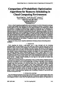
Data link layer is the second layer in the OSI-reference model provides services to network layer and control the physical layer. In resource management, the data link layer is responsible for bandwidth and channel allocation, scheduling, admission control, and network selection. They are described in the following. Admission Control The basic function of admission control is estimating the state of networks and then making decision if a traffic flow can be admitted. The objectives of admission control can be the optimal utility of networks, guarantee the QoE in the networks, load balancing, etc. The wireless access networks can have multiple classes of service, thus the admission control should have capability of distinguishing between them. Then, an appropriate amount of wireless resource can be assigned to the users. Call admission control schemes were mentioned in [57, 58, 43]. A call admission control for IEEE 802.11 single-hop networks with stochastic delay guarantees was proposed in [57]. While stochastic delay can be guaranteed successfully as shown in the performance evaluation, other parameters such as throughput and packet loss were not mentioned. The authors in [58] proposed an admission control scheme that combined with radio interface selection in heterogeneous wireless access networks. In [43], the authors consider call admission and hand-off between cellular and WLAN areas. When a new call occurs, the mobile terminal tries to connect to the cellular networks if there is no available resource in WLAN. For data traffic, the author in [59] proposed a distributed scheme of association in the wireless access networks. The algorithm copes with several different policies in wireless access networks: rate-optimal, throughput-optimal, delay-optimal, and load-equalizing. A degree of load balancing was proposed to switch between policies. To video streaming, the authors in [60] adopted PSQA tool to control flow admission at the AP in IEEE 802.11 networks. When a flow requires a connection, the AP will calculate MOS of ongoing streams. If the MOS of every stream is over the acceptable level plus a threshold, the new connection will be admitted. This is a reactive scheme that only launch if there is request of connection. However, the differentiated priorities of users were not addressed in this paper. Network Selection Different networks can coexist in the same region. When mobile users in an area of overlapping wireless access networks, their devices should detect and select appropriate networks automatically depending on requirements. This scenario has been motivating an enormous number of researches in network selection schemes. A brief summary of existing network selection schemes can be found in [61]. Existing approaches can be broken into three main groups: Multiple Attribute Decision Making (MADM), Game theory-based decision making, and QoE-based decision making. Fig. 1.1 describes the classification of existing network selection schemes. In MADM-based network selection schemes, each user adopts a joint metrics from different parameters to evaluate each network in its range. By comparing joint metrics of different networks, an appropriate network will be selected. Existing solutions in MADM

24

Chapter 1

EĞƚǁŽƌŬƐĞůĞĐƚŝŽŶ ƐĐŚĞŵĞƐ

DDͲďĂƐĞĚ

hƐĞƌƐǀƐhƐĞƌƐ

'ĂŵĞƚŚĞŽƌǇͲďĂƐĞĚ

hƐĞƌƐǀƐ͘ EĞƚǁŽƌŬƐ

YŽͲďĂƐĞĚ

EĞƚǁŽƌŬƐǀƐ EĞƚǁŽƌŬƐ

Figure 1.1: Classification of schemes in network selection problem group are Simple Additive Weighting Method (SAW), Technique for Order Preference by Similarity to Ideal Solution (TOPSIS)[62, 63], Multiplicative Exponential Weighting Method (MEW), Elimination and Choice Expressing Reality (ELECTRE), and Analytic Hierarchy Process (AHP) and Grey Relational Analysis (GRA). In [64], an access technology selection in heterogeneous wireless networks and a hybrid decision method were addressed. The proposed utility function comprises the cost and throughput. In [65], a radio access network selection scheme, which can facilitate seamless communications, joint resource management, and adaptive quality of service, was proposed. The proposed algorithm considers different user satisfaction functions involving resource utilization and the user satisfaction. In [66], an energy-aware utility function for user-centric network selection strategy and multimedia delivery in a heterogeneous wireless environment was proposed. Based on the mobile device type, application requirements, network conditions and user preferences, the proposed function selects a best value network which satisfies the user needs. The MADM group has several advantages such as consideration of multiple criteria and easy implementation. However, each solution is only suitable for a unique type of services. A detailed comparison of solutions in MADM group can be found in [67]. An alternative decision making in network selection is game theory-based approaches. Existing researches in this group can be broken into three types based on the players: users and users [68, 69, 40], networks and users [70, 71], networks and networks [72, 73, 74]. Furthermore, they could be classified according to the strategy of players. There are two strategies: cooperative strategy and non-cooperative strategy. Table 1.1 summarizes existing game theory-based network selection approaches. Scheduling Scheduling is one of the popular methods to distribute resources in wireless access networks. By scheduling, each user is able to access a specific radio resource in a given period of time. The scheduling strategies in wireless networks can be divided into channel-unaware, channel-aware, and energy-aware types. Fig. 1.2 describes the classification of scheduling problems. Firstly, the channel unaware methods are based on the impractical assumptions such as time-invariant and error-free transmission. The resource requested by users can be served

25


Group

Paper

Users vs Users

[68]

Noncooperative X

[69] [40] [70]

X X X

Users vs Networks Networks vs Networks

Cooperative

[71] [72]

X

[73]

X

[74]

X

Utility Number of users at AP and distance from user to AP Fixed Connection fee and bandwidth Linear pricing and bandwidth QoS parameters: delay, jitter, throughput, and packet loss and Cost User and network payoff functions Throughput

X

Datarate, packet delay, and packet dropping rate Bandwidth

Table 1.1: Game theory based network selection schemes

^ĐŚĞĚƵůŝŶŐƐĐŚĞŵĞƐ

ŚĂŶŶĞůƵŶĂǁĂƌĞƐĐŚĞŵĞƐ

ŚĂŶŶĞůĂǁĂƌĞƐĐŚĞŵĞƐ

KƉƉŽƌƚƵŶŝƐƚŝĐƐĐŚĞĚƵůŝŶŐ

ŶĞƌŐǇĂǁĂƌĞƐĐŚĞŵĞƐ

ĞƚĞƌŵŝŶŝƐƚŝĐ^ĐŚĞĚƵůŝŶŐ

Figure 1.2: Classification of schemes in scheduling problems

26

Chapter 1

in First In First Out (FIFO) manner. However, this method is unfair and inefficient in wireless networks, which have different classes of users and services. Another method is the Round Robin (RR). RR offers a fair approach to deliver resource to users. Because of non-deterministic conditions of wireless environment, the throughput of each user can be quite different even though every user is assigned the same amount of time. To address the throughput fairness, the Blind Equal Throughput (BET) was proposed in [75]. The users that had lower throughput than other users will be allocated more frequently than others to achieve better throughput. In the networks with different priorities of users, the resource pre-emption method can be adopted to support QoS flows in which the high priority flows (QoS flows) can occupy the resource of lower priority (non-QoS) flows. An alternative way to embed the priority into the flows is weighted fair queuing where a weight is assigned to each flow corresponding to its service. However, the above methods cannot guarantee the delay that can be required by applications. The earliest deadline first (EDF) and largest weighted delay first (LWDF), which are defined for wired networks and operating systems [76, 77], can be applied to the wireless networks. The next group of scheduling approaches is channel-aware group which takes into account throughput, time, and frequency. This group involves opportunistic scheduling and deterministic scheduling. Time-slots for each transmission in opportunistic scheduling are determined by stochastic approaches while deterministic scheduling provides exact time-slots for each transmission. Table 1.2 summarizes scheduling schemes mentioned in this section. The maximum throughput (MT) strategy aims to maximize the overall throughput of cells. This approach, however, can lead to an unfair resource distribution problem because the users with low quality of wireless channels can be assigned a short period to access the channel. Consequently, a combination of MT and BET, such as proportional fair (PF) scheduling, can be implemented to achieve both high utilization and fairness between users in cells. An optimization problem of assigning scheduling blocks and modulation and coding scheme (MCS) based on PF was proposed in [78]. Based on wireless channels feed-backs, an appropriate MCS and scheduling block will be assigned to the user in order to maximize the throughput in the networks with the PF manner or max-rate manner. However, the high computational complexity of integer linear programming of the proposed algorithm can lead to impractical implementation. Game-based strategies are another promising solutions because of their moderate complexity and high accuracy. In [79], the up-link scheduling in LTE problem was formulated as a cooperative bargaining problem, where user’s goal is to maximize its own utility. A Nash bargaining solution was derived for the resource allocation problem under power transmission constraint. In the proposed game model, centralized scheduling model where the BS was assumed to enforce the cooperative solution was considered. Above scheduling approaches are in deterministic group. Now, opportunistic scheduling methods are discussed. The opportunistic scheduling mechanisms were proposed in [87, 84, 86, 85]. A distributed scheduling for uplink OFDMA was proposed in [84]. Based on their channel state on each sub-carrier, users are broken into three groups with different priority of transmission. The priority of users are given based on channel-state indicator derived from beacon signals. In [85], two modified PF scheduling schemes named proportional fairness in frequency (PFF) and proportional fairness in time and frequency (PFTF) combined with probabilistic interference avoidance scheme for multi-cell OFDMA networks was proposed. The BS are able to shutdown high interference sub-channel opportunistically, thus enhancing

27


Group Deterministic Scheduling

Paper [78, 80] [81] [82]

[79] Opportunistic Scheduling

[83] [84] [85] [86]

Inputs Scheduling blocks and MCS Data rate Channel condition, modulation and coding schemes, and power transmission Resource blocks and transmission power Location channel state Interference and transmission power Channel gain

Objectives maximize throughput Fairness Average packet delay

Maximize utility Maximize utility Fairness and throughput Maximize utility Throughput

Table 1.2: Scheduling schemes average cell throughput and cell energy efficiency. The drawback is the low utilization of wireless resources. In [86], a distributed opportunistic access schemes for single-carrier and OFDMA systems was proposed. By designing a novel back-off scheme utilizing the channel information, the multi-user diversity gain can be achieved. Besides, scheduling is able to enhance energy efficiency in the wireless networks. In LTE networks, enhancing energy efficiency solutions can be deployed at both eNodeB and user equipments (UEs). The authors in [88, 89] considered relationship between traffic, energy consumption, and environment impacts, which showed negative results. Therefore, the green networking have been receiving concerns from both network operators and researchers [90]. Another research confirmed that high data rate transmission can save energy of eNBs by switching them into sleep mode frequently [91].An alternative approach, named Bandwidth Expansion Mode, can be used to enhance energy efficiency of eNB in the low traffic scenarios [92]. Moreover, the energy efficiency can be improved when the resource allocation is implemented in time domain [93]. Bandwidth and channel allocation Recent bandwidth allocation schemes in both homogeneous and heterogeneous networks are discussed in this section. Table 1.3 summarizes existing bandwidth allocation schemes. In [94], the author suggested a resource allocation based on maximizing the weighted sum rate under a total power constraint. This approach does not guarantee fairness, since the users with the best channels get most of the resources. In homogeneous network, a novel allocation sub-channels to users in OFDMA networks were proposed in [95]. The problem were formulated as a cooperative game in which a pair of users will negotiate with each other to achieve an acceptable MOS level. The MOS was calculated based on packet error rate and bandwidth by adopting equations in [96]. Although the efficiency and fairness in the networks was addressed, the reaction of the proposed scheme to congestion was not

28

Chapter 1

studied. Moreover, using the objective approach to measure MOS can be inaccurate. The aforementioned scheme was built up on the assumption that QoE model and the type of traffic are known in advance. However, in incomplete information scenarios, both QoE models and type of traffic can be unknown. To address incomplete information scenarios, the authors in [97] proposed two algorithms based on stochastic analysis. The paper also studied on the unkown playout time. The authors proposed an online-test optimization strategy which spends a period of time at the beginning of streaming to determine QoE model. Then, it will optimize the total MOS of all users during remaining time. The longer time is used for testing, the shorter time is used for optimizing MOS. A new metric, named loss function, was introduced to measure the performance deterioration caused by mismatched QoE model. Consequently, the objective is to find a resource allocation strategy to minimize the supermum value of loss function. The first discussed scenario was that QoE model was given but the parameters was unknown. The author proposed dynamic resource allocation strategy (DRAS) to solve the problem in this scenario. The DRAS consists of 2 phases: test and optimization. In the first phase, the proposed scheme will learn the QoE model of users by testing different allocation resources Rn in test interval tn . Then, in the second phase, DRAS will seek the optimal resource solution. The second scenario was introduced with the assumption of unknown QoE model and playout time. The authors proposed Blind-DRAS(BDRAS) to address the problem. The test domain is larger than DRAS then 2 objectives: the test time must be long enough to have an accurate QoE, and reducing the test time will not lead to reducing accuracy significantly. Through mathematical analysis, the paper determined the upper bound of the loss in case of DRAS and BDRAS. Nowadays, mobile equipment can be equipped with two or more radio interfaces. To overcome the bandwidth bottle-neck, multi-homing is a promising solution. Multi-homing users can connect to different networks simultaneously so that the total bandwidth can be satisfied. In [42], the author proposed two algorithms to allocate bandwidth in heterogeneous networks containing MTs with single-network and multi-homing services. The first one is centralized optimal resource allocation (CORA). Resource management is controlled by a central entity which can be a device of network operator. The second one is decentralized sub-optimal resource allocation (DSRA) in which MTs play active roles in the resource allocation operation whether by selecting the best available wireless network for single-network services or by determining the required bandwidth share from each available network for multi-homing services. However, heterogeneous services and the cost of changing networks were not discussed in this paper. As a result, the paper [44] proposed a distributed algorithm so that each network/bs can perform its own resource allocation to support the MTs according to their services classes for multi-homing in heterogeneous wireless access networks. Each user is associated to a home network. The required bandwidth can be provided through multiple radio interfaces. The utility function was derived from the bandwidth and the cost of the allocated bandwidth. The problem was formulated as a mixed integer linear programming that aims to optimize the total utility function in a given area under constraints of bandwidth of BS/APs. A dual decomposition was adopted to form a distributed solution. Cognitive radio is one of promising solutions for higher radio bandwidth utilization and better quality of wireless applications [98]. A novel channel allocation scheme for the QoE-

29

Network Layer Resource Management

Wireless Networks Cellular networks

Paper

Decision

[94]

Data rate

[95]

Explicit QoE-based functions Implicit QoE-based functions Utility function based (cost and bandwidth) Utility function based (cost and bandwidth) Continuity of channels

[97] Cellular networks and WLANs

[42]

[44]

Cognitive radio networks

[99]

Single network X

Multihoming

Not mentioned Audio, Video, Best Effort Multimedia

X X X

X

Serives

X

Call

X

CBR, VBR

Multimedia

Table 1.3: Bandwidth allocation schemes driven multimedia transmission over the cognitive radio networks was proposed in [99]. The approach incorporates the perception multimedia quality of end users into the channel allocation design for the cognitive radio networks. The analytical and simulation results showed the proposed channel allocation scheme can significantly improve the multimedia QoE performance of the priority-based secondary users with respect to the MOS, PSNR quality, blocking probability, dropping probability and throughput. However, the mobility of nodes was not mentioned.

1.4


The concept of multi-hop networks brings benefits and challenges for applications. Recently, the model of multi-hop networking has been adopted by 5G consortium. Device to Device (D2D) communication is a component of 5G architecture [100]. In the multi-hop networks, the routing algorithms play a decisive role impacted to the performance. As of its importance, the network layer based resource management will be discussed in details in this section and will be the main focus of this thesis. Network layer is responsible for relaying packets from the source to the destination in

30

Chapter 1

multi-hop networks. Resource management schemes in network layer focus on determining the optimal end-to-end paths, which is the responsibility of routing algorithms. The existing routing algorithms could be divided into two groups according to route computation process: centralized and decentralized approaches.

1.4.1

Centralized approaches

In the centralized approach, the network is deployed with a central entity that is responsible for observing network status, determining the optimal or sub-optimal solutions, and enforcing routing decisions. In the following, a review of centralized routing algorithms is provided. Table 1.4 summarizes the centralized routing algorithms presented in this section with regard to technique used (Solution), metrics, support on mobility, cross-layer approach, and objective. The cross-layer column presents whether the proposed approach is a combination of routing and another resource management scheme from a different layer. An optimal joint conflict-free routing and scheduling for real-time traffic in wireless mesh networks was studied in [101]. The problem was formulated as mixed-integer non-linear problem (MINLP) that minimizes delay in the network. Because of high computational complexity of MINLP, the authors proposed a Lagrangian heuristic algorithm. The authors in [102] studied a joint routing and scheduling problems in wireless sensor networks. By adopting effective capacity (EC) model proposed in [110], the problem was formulated as a MINLP. The objective is to minimize channel usage subject to constraints on data rate, delay bound, and delay bound violation probability and restriction of network flow assignment. To overcome high computational complexity, the authors proposed a EC-based Column Generation Algorithm heuristic algorithm. The authors of [103] proposed a joint routing and scheduling for cognitive radio networks under uncertain spectrum supply in order to maximize system throughput. The problem is NP-complete and solved by an Iterative Linear Programming (ILP) based algorithm. A scheme for assigning relay nodes to enhance throughput in cooperative multi-hop networks was proposed in [107]. The objective is to maximize the minimum data rate in the networks by selecting the set of relay nodes. The problem was formulated as mixed integer linear problem (MILP). To address computational complexity, a combination of Branch and Bound - Cutting Plane (BB-CP) and Feasible Solution Construction (FCS) was exploited to achieve solution timely. All aforementioned routing algorithms does not consider multi-path routing which can split a stream among different paths to enhance utilization. To provide multi-path routing, the authors of [108] proposed an optimization architecture for joint multi-path and scheduling problem in wireless mesh networks. The paper adopted multi-commodity flow and time constraints proposed in [111]. Routing solutions are obtained by Proximal Optimization Algorithm. With similar network model, the authors of [109] addressed the video dissemination over hybrid cellular and ad-hoc networks. The problem was a joint routing and scheduling problem in order to maximize video quality. The video quality was computed by Rate-Distortion model [112]. Three algorithms have been proposed to obtain the solutions: Prioritized algorithm, maximum throughput scheduling algorithm, and tree-based heuristic algorithm. Both prioritized algorithm and maximum throughput scheduling algorithm are unable to tackle large-scale problem because they exploit numerical methods to solve optimization problem while tree-based heuristic algorithm can solve the

31


Paper

Solution

Metric

Mobility

[101]

Interference + Time slot Effective Capacity

No No

Scheduling

Minimize delay + maximize channel usage

[103]

Langrangian relaxation based EC-based ColumnGeneration Algo. ILP-based alg.

Cross-layer (Routing+) Scheduling

No

Scheduling

Maximize throughput

[104]

Dijkstra

No

Application

Video quality

[105]

Dijkstra

No

No

Video quality

[106]

Dijkstra

No

No

Video quality

[107]

BB-CP + FSC

Interference + Robustness + Link capacity Bandwidth + delay Throughput, loss rate, jitter, and QoE Interference and length Bandwidth

No

No

[108]

Proximal Optimization Algorithm Prioritized alg., maximum throughput scheduling, and tree-based heuristic algorithm

Bandwidth

No

Scheduling

Maximize minimum data rate Maximize bandwidth

Time slot + Bandwidth

Yes

Scheduling

[102]

[109]

Table 1.4: Centralized Routing schemes

Objectives Minimize delay

Video quality

32

Chapter 1

Network environment aware [114, 115, 116, 117, 118, 119, 120, 121, 122, 123, 124, 125, 126, 127]

Probabilistic [128, 129, 130, 131, 132]

Routing algorithms Graph-based Utility-based [133, 134, 135, 136, 137, 138]

[12, 13, 14, 139, 140, 141, 142]

Learning-based [143, 144, 145, 146, 147, 148, 149, 150]

Table 1.5: Decentralized Routing schemes problem in real-time. The software-define networking paradigm unveil a novel application of centralized routing algorithms [113]. In [104, 105], routing algorithms for streaming SVC over SDN was proposed. In [104], the cost of link consists of the ratio of the required bandwidth and the available bandwidth and the delay. As the required bandwidth for different layers are not the same, the cost of link for different layers are not the same. Subsequently, the end-to-end path for each layer is determined by using Dijkstra algorithm. Similarly, [105] adopted constrained shortest path first to determine the end-to-end paths that satisfy given requirements of throughput, loss rate, and jitters. It is worth noting that the algorithm takes quality of experience (QoE) into account. The value of QoE metric are monitored and a new path is determined when there is degradation of QoE metric. The authors in [106] proposed a routing algorithm that take interference into account. The cost of a path is the ratio of the number of nodes interfere with this path and the number of relaying nodes. The chosen path is the path with the lowest cost.

1.4.2

Decentralized approaches

The centralized schemes have been discussed in the previous section. In this section, decentralized routing algorithms are discussed. Because of the distributed nature of the Internet, decentralized routing algorithms outnumbers centralized routing algorithms. Decentralized algorithms are the routing algorithms in which routing decisions are computed selfishly or cooperatively without coordinating of any central entity. In this section, a comprehensive review of decentralized routing algorithms is provided. They are able to classified into six major categories: Network Environment Aware, Stochastic, Graph-based optimization, Utility-based optimization, and Learning-based optimization. Table 1.5 presents the taxonomy of decentralized routing algorithms. 1.4.2.1

Network Environment Aware routing algorithms

The network environment aware routing algorithms take one or multiple network-related metrics, such as location of node and link quality, into account. This group is able to be divided into two sub-groups: geographic routing and link quality aware routing. Geographic routing computes the routes based on location of nodes in the networks. Meanwhile, link quality aware routing give routing decision based on quality indicators of links.


33

Geographic routing algorithms are dynamic and topology-independence, thus it is suitable for the lack of infrastructure in Ad-hoc networks. In [114], the author proposed Greedy Perimeter Stateless Routing (GPSR). The positions of nodes are exploited to select forwarders. Greedy forwarding algorithm in GPSR guarantees that packets always move towards destinations progressively. When a greedy path does not exist, GPSR recovers by forwarding in perimeter mode. The perimeter mode drives packet to faces of a planar subgraph of the full radio network connectivity graph. When packets reach a node closer to the destination, the greedy forwarding resumes. The authors in [115] proposed another geographic routing algorithm for streaming H.26L video over wireless networks. The algorithm defined the reference line as the straight line between the origin of the virtual coordinate system to the destination, then deviation angle describes how much a path is expected to deviate from the reference line at the origin point. The multiple disjoint paths with lowest deviation angle values facilitates load balancing, bandwidth aggregation, and fast packet delivery. In [116], a geographic opportunistic routing algorithm was proposed. The forwarder selection is selected opportunistically. To begin, the source sends a Request To Forward (RTS) packet broadcast. The neighbors contend to each other by replying a Clear To Forward packet (CTF). CTF packet transmission is scheduled by a distance-based timer. Subsequently, the fist node replying to the source is selected as the forwarder. The aforementioned geographic routing algorithm does not take link quality into account, thus it may not applicable in high traffic wireless networks. To address this drawback, the Cooperative Opportunistic Routing Protocol (CORMAN) proposed in [117] determines routing decision based on the link quality extracted from Received Signal Strength Indicator (RSSI). In essence, the radio transmission range is described by irregular shapes because of the variation of the signal quality. By collecting information from PHY layer, both packet delivery ratio and throughput are better than the conventional geographic routing solutions. A routing algorithm for Internet of Things application was presented in [118]. The idea of Dynamic Forwarding Delay introduced in [151] has been adopted. The source broadcasts the data packet, then all possible forwarders determine DFD timer based on local information. When DFD timer expires, the packet is forwarded. Other forwarders which are aware of the occurrence of relaying cancel the scheduled transmissions for the same packet. The DFD in [118] differs from the original idea, which computes DFD on the distance to the destination. It is determined by a combination of link quality, distance to the destination, and remaining energy. The drawback of geographic routing is that geographic information is not correlated to link status, such as signal strength and length of queue. In fact, the status of a link defines the delivery ratio, then impacting to general performance of the networks. The following routing schemes use a joint metric of location and link quality so as to compute routing decisions. In [119], a new anypath routing scheme for prolonging the path lifetime was proposed. In contrast to unicast routing, the packet will be forwarded to a forwarding set instead of a single neighbor. For each forwarding set, relay priority of a vehicle is determined based on a weighted sum of all paths to destination, which is derived from the packet loss rate and the relative distance of nodes belonging to the paths. The authors of [152] proposed a joint routing and scheduling, named the Multiple access scheduling in Multi-radio Multichannel Mesh networking (M4). The radio and channel schedules are determined by using

34

Chapter 1

compact Latin square in order to achieve efficiency and fairness. For routing aspect, a proposed metric, named forwarding speed, was utilized to evaluate paths. Forwarding speed is the ratio between the geographic distance and the access delay (queuing delay and medium access delay). The path with the greatest forwarding speed is chosen. The drawback of both routing scheme is that they require geographic information of other nodes, which may not be available and has to be obtained by exchanging control messages. To avoid the need of geographic information, some routing schemes compute routes based on other metrics. In [121], each node compute trusts value for each neighbor. Trust value is the ratio of the number of correctly forwarded packets and the number of successful received packets. The routing cost metric of a route is computed by the total delay of a packet and the trust value. A multi-hop multipath heterogeneous connectivity (MMHC) routing algorithm proposed in [123]. Three characteristics including mobility of intermediate nodes, throughput of links, energy of intermediate nodes were considered. The study considered routing with different objectives: shortest path, maximum throughput, energy fairness based on average path energy, and mixed strategy. The proposed algorithm can be extended by adopting the QoE to select the path. In [120], each mesh router is equipped with a E-Mesh route information collector and E-Mesh route selection. E-mesh route information collector module is responsible for gathering data (remaining energy, current load, and node position) extracted from Announcement Traffic Indication Message (ATIM) packets. E-mesh route selection calculates the utility based on information storing in E-mesh route information collector. In [124], the authors proposed a routing scheme for video streaming, named Fieldbased anycast routing (FAR). The selection path algorithm of FAR is inspired from the electrostatic field characteristics where a positive electron moves from a high potential point to a lower one. The potential of each node is determined based on neighbors’ potential and the length of its queue. Each packet, which acts as a positive electron, flows through nodes in the mesh network until it reaches the sink. 1.4.2.2

Probablistic approach

The unpredictable mobility in mobile Ad-hoc networks causes difficulties in selecting the forwarders. Probabilisitc routing algorithms address that challenge by adopting statistical tools to predict the availability and quality of relaying candidates. In [128], the authors proposed Delegation Forwarding, a probabilistic routing protocol for Mobile Ad-hoc networks. By observing the connection of a node, Delegation Forwarding is able to derive the contact rate, then making forwarding decisions. Delegation Forwarding can reduce the number of message replicas compared to greedy forwarding. While Delegation Forwarding generates message replicas statistically based on the encountered node utility, sources in Optimal probabilistic forwarding (OPF) [129] are able to duplicate a given packet and choose multiple relaying node to forward it. The forwarding process was modelled as an optimal stopping rule problem in order to maximize the expected delivery ratio. OPF also defines the forwarding threshold that are a function of remaining hop-count and time-to-live so as to limit the route length. Other variants of OPF, named OOF and OOF-, have been presented in [130]. OOF enhances the computation of the packet delivery probabilities in [129], thus maximizing the expected packet delivery. Meanwhile, OOF- aims to minimize the delay. The expected delay metric, similar to the expected delivery metric, is computed

35


Paper [114]

[116]

Solution Greedy forwarding Greedy forwarding -

[117]

-

[118]

Dynamic forwarding delay

[119]

-

[120]

-

[121]

-

[123]

-

[124] [152]

Field-based Forwarding speed

[115]

Metric Geo. position

Mobility Yes

Cross-layer No

Objectives Geo. distance

Geo. position

Yes

No

Geo. distance

Geo. position + Link quality + Residual energy Hop count + RSSI Geo. position + Link quality + remaining energy Loss rate + geo. distance Geo. position + Current load + remaining energy Delay + Link reliability mobility + throughput + energy queue length Delay + Geo. position

Yes

Scheduling

Geo. distance + Reliability

Yes

No

Yes

No

Overhead + Robustness Reliability + Throughput

Yes

No

Reliability

Yes

No

Video quality

Yes

No

-

Yes

No

Energy + throughput

No No

No Multi-radio + multi-channel + Scheduling

Video quality throughput + delay

Table 1.6: Network environment aware Routing algorithms

36

Chapter 1

Paper [128]

[131]

Analytic tool Optimal stopping theory Optimal stopping theory Optimal stopping theory -

[132]

-

[129] [130]

Metric Quality

Mobility Yes

Cross-layer No

Objectives Delivery ratio

Packet delivery rate Packet delivery rate + delay Geo. position + Tx power ETX + remaining energy

Yes

No

Delivery ratio

Yes

No

Yes

No

Yes

No

Delivery ratio + delay Reliable broadcast Network life time

Table 1.7: Probabilistic routing algorithms based on the inter-meeting times estimates, therefore lower delay can be obtained. In [131], the authors proposed Collision-aware reliable forwarding (CAREFOR) for VANETs. The stochastic broadcast scheme of CAREFOR helps reducing the required number of rebroadcasts in order to forward a packet to a destination. CAREFOR comprises two phases: a collision probability estimation phase and a reliable forwarding phase. To begin with, a source sends a Request-To-Broadcast (RTB) packet, which consists of the position of the node, the density, and the transmission power, to all nodes in its vicinity. A nodes that receives RTB estimates the collision and assesses if it is qualified for reliable forwarding phase. A qualified node sends Clear-To-Broadcast (CTB) packet to the source in order to confirm the qualified rebroadcast forwarder. The authors of [132] proposed a routing algorithm that takes into account both remaining energy and link quality. To assess link quality, Expected tranmission count (ETX) has been adopted, then the forwarding probability is a function of ETX and remaining energy. EEPR can achieve longer network life time compared to AODV. However,both routing setup delay and routing success probability are lower than AODV. 1.4.2.3

Graph-based optimization routing algorithms

In conventional routing protocols, the shortest path among available paths is chosen. The cost can be the number of hops from the source to the destination. Ad-hoc On-Demand Distant Vector (AODV) [133] and Optimized Link State Routing Protocol (OLSR) [134] are the most well-known protocols exploiting this metric. A multipath extension of OLSR was presented in [135]. Multiple end-to-end paths are determined explicitly at the source by Multipath Dijkstra Algorithm. Though the routes in MPOLSR are not computed distributedly, the distributed selection of Multipoint relays (MPRs) puts MPOLSR into decentralized group. Another variant of OLSR, named crosslayer QoS-aware routing protocol on OLSR (CLQ-OLSR), has been introduced in [137]. Two sets of routing mechanisms were implemented, physical modified OLSR protocol (M-OLSR) and logical routing, by constructing multi-layer virtual logical mapping over physical topol-


37

ogy. Physical M-OLSR protocol is responsible for routing table construction and bandwidth estimation on best-effort interface, while logical routing on real-time interfaces computes the optimized logical path from topology and bandwidth information. Every node in CLQ-OLSR estimates the available bandwidth on each associated channel. Each node disseminates information of topology and available bandwidth to other nodes through HELLO and TC messages. The optimized logical path could be computed from the topology and bandwidth information. CLQ-OLSR outperforms OLSR [134] and multichannel-OLSR [153] in terms of average packet delivery rate, delay, and jitter. Multipath versions of AODV were studied in [154, 155, 156, 136]. AOMDV [154] extends AODV to discover multiple link-disjoint paths between the source and the destination in every route discovery. AODV control packets were modified with few extra fields in the packet header such as advertised hop count and route list. The main drawback, which is called "route cutoff" in AOMDV, is that it cannot find both of the reverse paths when there are one or more common intermediate nodes in a pair of link-disjoint paths. It is necessary to search for all of the existing link-disjoint reverse paths in order to reduce route discovery latency. The authors of [155] proposed an optimization AOMDV (OAOMDV) to tackle the "route cutoff" problem in AOMDV. Control packet RREP _ACK, which has been defined in AODV, was redefined in order to form a new reverse path. Although the proposed routing scheme OAOMDV increases an additional routing packet, simulations show that the routing overhead is decreased. Packet loss, route discovery frequency, and average end-toend delay also has been improved. An extension of AOMDV for multi-interface and multichannel networks, named (Extended AOMDV for Multi-Interface Multi-Channel networks) EAOMDV-MIMC, has been studied in [136]. The algorithm starts with estimating the average queuing delay for each channel. Based on that estimation, the forwarder is selected. That algorithm outperforms conventional AOMDV. The aforementioned routing algorithms are designed for general data networks. Next, we are going to introduce some video-aware routing algorithms. A reactive QoS-aware routing was proposed in [138]. The routing algorithm introduced an estimation of video session bandwidth which is broadcast by route request messages. When a node receive a request message, it will check if it can provide the required bandwidth and inform it the sender. This routing algorithm also supports multiple paths in order to alleviate route failures. A QoS-based routing for video streaming over SDN was proposed in [122]. The cost metric is a weighted combination of packet loss and delay variation. The proposed algorithm is to find out the minimum cost route satisfying a given maximum delay variation. By separating a network into multiple domains, the complexity of proposed algorithms solely depends on the number of border nodes. 1.4.2.4

Utility-based optimization routing algorithm

In this section, the routing problems are formulated into optimization problems in which the objective is to optimize the utility function. The optimization problem could be solved by adopting optimization tools, such as optimization programming and game theory. In [12], a resource allocation in network layer for surveillance camera application was proposed. A monitoring system including multiple cameras deployed over flexible and lowcost multi-hop wireless networks was considered. Three approaches were proposed including

38

Chapter 1

Paper [133] [134] [135] [136] [137] [138] [122]

Analytic tool Bellman-Ford Dijkstra Multipath Dijkstra Bellman-Ford Dijkstra

Metric Hop-count Hop-count Hop-count

Mobility Yes Yes Yes

Cross-layer No No No

Queuing delay Bandwidth

Yes Yes

No No

Dijkstra Constrained Shortest Path

Bandwidth packet loss + delay

Yes No

No No

Objectives Shortest path Shortest path Multiple disjoint paths Multiple paths Multiple paths + bandwidth Video quality Video quality

Table 1.8: Graph-based routing algorithms a centralized optimization, a decentralized game-theoretic, and a distributed greedy ones. Performances of proposed approaches were compared through four metrics: total video quality, computational complexity, and control information overhead, timely adaptation to the network and source variation. In [13], routing problems are formulated as bi-criteria routing games in which players want to optimize both congestion and path lengths. C+D games, Quality of Experience (QoE) games, and max games were studied. The C + D have games instances that do not stabilize. Quality of Routing (QoR) games stabilize and their equilibria provide good approximations to the C + D optimization problem. Max games stabilize and have price of stability 1, the best possible, however the price of anarchy may be large. Time efficiency of proposed solutions, however, was not mentioned in the paper. In [14], a routing problem for video surveillance in vehicular sensor networks was formulated in the form of Bayesian coalition game. The players in the game are learning automata stationed on the vehicles. Through the cooperation between players, the optimal number of video flows can be achieved. The authors of [140] formulated the routing problem as a utility maximization problem. A game-theoretic approach has been adopted to optimize routing decisions and rate allocation for multiple flows. Source nodes were formulated as both cooperative and selfish players. Each player performs local optimization and derives the iterative rules, which indicates the encoding and broadcast rates to be assigned to the source and relaying nodes. While selfish players attempt to optimize their own payoffs, the objective of cooperative players is to optimize social payoff through a decentralized bargaining algorithm. Similar to [140], the routing problem was formulated as a utlity maximization problem. Each relay in [139] is assigned a Residual Expected Network Utility (RENU) value, which is a function of the benefit of successful packet delivery and transmission cost. The routing algorithm, subsquently, attempts to maximize the utility so as to maximize the reliability of the networks. The authors in [141] studied the routing problem in multiple simultaneous sessions. This problem was formulated as a convex optimization problem. The utility is an increasing strict concave function of allocated information rate. The proposed algorithm, named Consort, is a message passing algorithm. The original problem is broken into subproblems by using Lagrangian method. Consequently, each node can solve its own sub-

39


Paper [12]

Analytic tool Game theory

Metric Bandwidth

Mobility No

Cross-layer No

[13]

Game theory

Queue length + Bandwidth

No

No

[14]

Game theory

Bandwidth

Yes

No

[139]

Exhaustive serach Game theory

Residual utility

No

Scheduling

Geo. distance

No

Lagrangian method Floyd Warshall algo. Lagrangian method

Bandwidth

No

Network coding + scheduling No

Delivery delay

Yes

No

Energy + Link quality

No

No

[140] [141] [142] [150]

Objectives video quality + overhead Reduce congestion and path length Number of video flows Reliability Maximize data rate Delay Energy efficiency + bandwidth

Table 1.9: Utility-based routing algorithms problem with its local information and updated Lagrange multiplier, then exchanging the solution with others to obtain a consensus. Consort [141] outperforms Dice [140] in terms of fairness and node load violation ratio. To address delay-sensitive applications, the authors of [150] proposed a joint routing and power control scheme. The goal of proposed scheme is to enable a node to choose a forwarder that offers a higher successful transmission rate. To address the delay, the authors of [142] proposed a Time-sensitive Opportunistic Utility-based Routing Protocol (TOUR) for Delay Tolerant Networks. TOUR is able to forward a packet through a short-delay yet costly path statistically. Each packet is assigned with a initial benefit that are up to its important. This benefit degrades with time. The utility for each packet is the gap between the benefit and the transmission cost. The algorithm also introduces the concept of time-varying optimal forwarding in order to tackle the time varying benefits and dynamic topology. 1.4.2.5

Learning-based optimization routing algorithm

The aforementioned algorithms do not mention time-varying link quality, which impacts directly to forwarder selection. It is assumed that the probability model of wireless connections and local network topology are known precisely. Learning theory is a prospective approach that lets the wireless node adapt their routing decision to dynamically environment efficiently. The authors of [146] proposed a reinforcement learning geographic routing scheme that increases packet delivery rate and network lifetime in wireless sensor networks. A node selects

40

Chapter 1

Paper [146]

Analytic tool RL

[148]

MARL

[147] [149]

MARL + decay function MDP

[143] [145]

RL Nash-Q learning

Metric Expected retransmission Mobility + Congestion + Buffer Link stability

Mobility No

Cross-layer No

Objectives Reliability

Yes

No

Reliability

Yes

No

Reliability

Residual energy

No

No

PDR Residual energy + PDR

No Yes

No Scheduling

Delay-sensitive applications Reliability Delivery ratio + Energy efficiency

Table 1.10: Learning-based routing algorithms a forwarder according to the expected number of retransmission along a route. The authors of [143] proposed, AdaptOR, an adaptive routing protocol. The objective is to minimize the average per packet routing cost without knowledge of network topology and link quality. The probabilistic model in AdaptOR are learned dynamically using a reinforcement learning. The learning process depends on the exchanging control packet process, thus the loss of control packet degrades the performance of AdaptOR. In [149], a Markov Decision Process (MDP) model Q-routing approach, named QELAR, was proposed in order to reduce and balance energy consumption. A node selects a relaying node according to the residual energy. The rewards represent transmission energy and residual energy incurred for forwarding the packet. Above routing algorithms provide local optimization regardless of the global performance, thus they are not appropriate to obtain global optimization. Multi-agent reinforcement learning (MARL) can overcome this drawback by enabling neighbors to exchange local observed information. Through collaboration, the global optimization can be achieved. In [148], a MARL based routing algorithm, named Adaptive reinforcement-based routing (ARBR), was proposed. The objective of ARBR is to select a reliable forwarders among neighbors. Three main factors (node mobility, congestion level, and buffer utilization) were taken into account. The collaboration is done by exchanging reward value with one-hop neighbors. Instead of reward value exchange, the MARL-based routing algorithm in [147], named SAMPLE, adopted decay function concept. Neighbors cooperate through exchanging route cost advertisements. The route cost comprises a decay function and rewards. The rewards represent the link stability while the decay function increases if it is not updated within a time window. A joint directional routing and scheduling for vehicular delay tolerant networks, named directional routing and scheduling scheme (DRSS), was proposed in [145]. The Nash-Q learning approach was utilized to find the optimal routes with the unknown network environment. The simulation results showed that both energy efficiency and delivery ratio could be improved.

Conclusions

41

Numerous research works have been conducted in routing over wireless networks for multimedia streaming, nevertheless the users’ experience has not been considered appropriately. Consequently, a routing protocol that takes real users’ experience into account has been considered in this thesis.

1.5

Conclusions

The objective of this section is to provide a brief summary of existing resource management solutions, especially on network layer. We divided into two groups: upper-layer and lower-layer. In upper-layer group, solutions are to manage cache memory and congestion window. Meanwhile, the lower-layer group control resources by enforcing data-link layer and network layer. Motivated by the advantages of WMNs, this thesis focuses on network layer resource management scheme. One of the most important components of network layer resource management scheme is the routing algorithm. The existing routing algorithms can be classified into two major groups: centralized and decentralized. In the centralized group, a central entity is responsible for determining the routing decisions after collecting network status from other nodes. In contrast, the decentralized group consists of algorithms in which each node gives decision selfishly based on its awareness. Although a number of studies have been conducted to manage resources in wireless networks, most of them are based on QoS metrics to control resources and evaluate performance. However, it has been demonstrated that the QoS metrics may not correlate well with the experience of users. As a result, QoE-based resource management schemes attract interest from both researchers and engineers. Consequently, this thesis adopt QoE assessment as routing metric instead of or in addition to other network-oriented metrics.

42

Chapter 1

Chapter 2

QoE models and estimations 2.1

Introduction

In this dissertation, QoE metric is exploited to compute routing decisions. Consequently, it is important to provide details of the models that are used for an accurate and online estimation of QoE metric. A brief background of video coding standards and quality assessment methods are presented in this chapter. Nowadays, H.264 video coding standard and its variations are one of the most popular video codecs used in video streaming services. The standardization of H.264 was completed in 2003. Then, an important extension of H.264, Scalable video coding (SVC), was introduced in 2007. This dissertation focuses on H.264 and its extension SVC. Therefore, both of them are reviewed in this chapter. Later in this chapter, quality assessment methods are discussed in order to provide the motivations for using QoE into routing algorithms. QoE models are presented in implicit mathematical forms, then their approximations are proposed. The characteristic of approximations are also provided in this chapter. The remaining of this chapter is organized as follows. The chapter begins with a brief review of H.264 video coding in Section 2.2. Subsequently, existing quality assessment methods are discussed in Section 2.3. It is followed by approximations of PSQA models described in Section 2.4 and Section 2.5. The conclusions of this chapter is provided in Section 2.6

2.2 2.2.1

Video Coding H.264

H.264 is an open, licensed standard that provides the efficient video compression techniques. As compared to previous codecs, it allows streaming and storage of videos while taking less bandwidth as well as less storage space without attenuating image quality. Fig. 2.1 shows that the bit rate generated by H.264 encoder is up to 50%, 70%, and 80% lower than MPEG43

44

Chapter 2

Figure 2.1: Bit rate generated by H.264 baseline profile, MPEG-4, and Motion JPEG [157] 4 encoder with motion compensation and without motion compensation and MotionJPEG encoder, respectively. A video codec has a pair of algorithms that are responsible for compressing and decompressing a given video. Note that different video codec standards are not compatible with each other. An important feature of H.264 is enabling multiple profiles and levels that support different goals and devices. H.264 has seven profiles and eleven levels. While a profile defines the feature set used by the encoder and the complexity of the decoder, a level defines the bitrate and the encoding rate for various resolutions. There are three main types of frames in H.264: I-frames, P-frames, and B-frames as shown in Fig. 2.2. Moreover, the encoder can send Instantaneous Decoder Refresh (IDR) frame, which is a special type of I-frame in order to specify that no frame after the IDR frame can reference any frame before it. This frame helps to seek the H.264 file easier and more responsive in the player [158]. The ratio between different types of frames is up to the profile. • I-frame, or intra-coded frame, is a self-contained frame and can be decoded independently. It marks the starting point for new viewers or the re-synchronization point in case the transmitted bitstream becomes corrupted. I-frames use many more bits than other frames. • A P-frame, or predictive inter frame, uses prior I and/or P-frames as references, thus requiring the decoding of previous pictures to decode itself. P-frames consume fewer bits than I-frames, but they are sensitive to losses. • A B-frame, or bi-predictive inter frame, uses both an earlier and a future frame as

45

Video Coding

Figure 2.2: A sequence of H.264 frames [157]

Figure 2.3: Difference encoding [157] references. H.264 utilizes temporal redundancy elimination by encoding only the delta, or the difference, between the current frame and the referenced frame. Only pixels that have changed with respect to the reference frame are encoded. Fig. 2.3 depicts the principle of this type of encoding and lets call it as difference coding. However, difference coding may not significantly compress a video when there is a lot of motion in the video. In such cases, block-based motion compensation can be exploited. Block-based motion compensation (BMC) technique divides a frame into macroblocks. A new frame can be predicted by looking for the matching block in a reference frame even if it moved to a different location in the current frame. The motion vector shows the moving of the block. The motion vector consumes fewer bits than coding the content of the block. Fig. 2.4 depicts the operation of BMC.

2.2.2

Scalable video coding

Recently, H.264 has been extended to enable scalable video coding (SVC). This allows the deployment of advanced applications, such as scalable video streaming and universal multimedia access. In SVC, a high quality video bitstream can be encoded to contain one or more sub bitstreams. A sub bitstream, also called as a layer, can be derived by discarding packets from the higher bitstreams. The quality of video is dependent on the number of received layers.

46

Chapter 2

Figure 2.4: block-based motion compensation [157]

Figure 2.5: SVC scalabilities [159]

Quality assessment

47

There are three types of scalabilities in SVC: spatial, temporal, and encoding quality as shown in Fig. 2.5. SVC videos consist of a base layer and multiple enhancement layers. The base layer is H.264/AVC compliant so as to enable backward compatibility. Spatial and temporal enhancements can be obtained by receiving enhancement layers with improved picture size (spatial resolution) or frame rate (temporal resolution), respectively. The encoding quality enhancement can be achieved by receiving enhancement layers with a finer quantization step-size than the base layer. One or multiple enhancement layers can be be removed in order to adapt to the bandwidth limitations in wireless networks.

2.3

Quality assessment

In recent years, there is an increasing recognition that QoE metrics are more pertinent to evaluate the quality perceived by users. While the network-oriented parameters, such as delay, jitter, packet loss, etc. are the fundamental metrics in QoS schemes, the QoE is based on feelings of users. Although a better network QoS can lead to better QoE, fulfilling all QoS parameters may not guarantee a satisfied user. Moreover, even with a bad QoS metrics, good QoE, in fact, can be achieved [160]. Subsequently, QoE attracts significant attention from both industry as well as academy. As a result, ITU standardization bodies spent a significant effort to the QoE and related issues. The ITU-T Study Group 12 (SG12) develops international standards on performance, QoS and QoE. It defines a large number of high priority questions that are being addressed in collaboration with several ICT (Information and Communication Technologies) partners. QoE has been defined by ITU as follows: "QoE is a measure of the overall acceptability of an application or service, as perceived subjectively by end-user". Thus, QoE considers factors related to both the services and users. The service factors include availability, reliability, set-up and response times, type of terminals, etc. Meanwhile, the users’ factors consist of emotions, experience, motivation, and goals. The QoE measure has a distinct meaning according to the specificity of each application. A positive QoE measure in voice services, for example, signifies that the call is characterized by an excellent voice transmission quality and low probability of blockage. Nevertheless, a positive QoE measure in Web surfing applications can be achieved when good quality graphics and pictures are downloaded within an acceptable period of time. The video quality measurement can be done using either objective or subjective approaches. In the objective approaches, explicit functions of measurable parameters can be exploited to evaluate satisfaction of users. Meanwhile, the subjective methods are based on evaluations given by humans based on their perceptions under proper definitions and conditions. The main drawback of objective approaches is that they may be uncorrelated with human perception. The mean square error (MSE) or peak signal-to-noise ratio (PSNR) are popular objective approaches. Furthermore, other computationally intensive methods for objective evaluation such as the moving picture quality metric (MPQM) and the normalized video fidelity metric (NVFM) were proposed. Recently, the initial waiting time and probability of interruption in video streaming were taken into account for QoE measurement [47]. On the subjective quality-assessment methods, the mean opinion score (MOS) recommended by the ITU is the common tool for video quality measurement. Even though

48

Chapter 2

MOS studies have provided fundamental concepts for analyses through signal processing, still there are significant limitations: very stringent environments are required, the process cannot be automated, and it is very costly and time consuming. Consequently, MOS evaluation is impossible to be conducted in real-time. To address the above limitations for MOS evaluation in real-time, Pseudo-Subjective Quality Assessment (PSQA) is a promising solution. PSQA is based on statistic learning using random neural network (RNN), as proposed in [161]. The methodology used by PSQA for QoE evaluation can be found in [18].

2.4

Loss rate and mean loss burst size-based QoE model

A hybrid method for measuring MOS, named Pseudo-Subjective Quality Assessment (PSQA), was proposed in [18]. PSQA uses random neural networks to determine a mapping between network-oriented metrics and MOS. The two QoS metrics are end-to-end loss rate (LR) and mean loss burst size (MLBS). Mean loss burst size is the mean of the numbers of consecutive loss packets in a stream. Let us denote U () is the implicit function of the PSQA model. Two arguments of U () are the loss rate Λ(d) and the mean loss burst size M (d) , where d is the stream index. In other words, the MOS of stream d can be determined by Ψ(d) = U Λ(d) , M (d) . (2.1) Estimations of the arguments and the implicit function U () are discussed in the following parts.

2.4.1

Estimation of the arguments

Each stream corresponds to a destination, so the stream index and the destination index can use interchangeably. Consider a path i from source s to destination d, Pi (s, d), which consists of several different nodes. The loss rate is measured every τ (window length). We have the LR over Pi (s, d) during window k can be given as follows. Y (1 − LRv (k)). (2.2) LRe2e Pi (s,d) (k) = 1 − v∈Pi (s,d)

The LR in two-hop can be derived in every window, however it is non-trivial to derive the end-to-end LR. To measure the end-to-end LR, the source node has to collect LR information of all intermediate nodes in the paths which is infeasible in wireless mesh networks. From (2.2), we have e2e LR2hops Pi (s,d) (k) ≤ LRPi (s,d) (k),

(2.3)

where LR2hops Pi (s,d) (k) is the first two-hop LR. Beside LR, the mean loss burst size (MLBS) is one of the input metrics impacting the MOS. The Gilbert model (see Fig. 2.6) was adopted to express the burst loss on a link em with pem and qem are the probability of link em changes from good to bad state and vice versa, respectively.LRem and GRem are distributions of bad and good states of link em .


49

Also, the Gilbert model was utilized to model the burst loss of outgoing packets at node i with pi and qi are the probability of the transmission changes from good to bad state and vice versa, respectively. LRi and GRi are distributions of bad and good states of node i. Assuming that there are n packets at node i. A packet a was successfully forwarded on link em . There are two situations can happen to the next packet b. • The next packet is going to be forwarded on the same link em . The next packet will be corrupted if the link em switches to the bad state. The probability of this situation is X sem →em pem (2.4) em

where sem →em is the probability of packet a forwarded on em and b forwarding on the same link. • The next packet is going to be forwarded on another link ek . The next packet will be corrupted if a loss happens on link ek . X X sem →ek LRek

(2.5)

em ek 6=em

where sem →ek is the probability of packet a forwarded on em and b forwarding on ek Then, we have the probability of transmission at node i changes from good state to bad state as follows   X X sem →em pem + (2.6) pi = sem →ek LRem  em

ek 6=em

Similarly, we have the probability of transmission at node i changes from bad state to good state as follows   X X sem →em qem + qi = sem →ek GRem  (2.7) em

ek 6=em

The distribution of bad and good states of node i are LRi (k) = πi0 (k) =

qi (k) , pi (k) + qi (k)

(2.8)

GRi (k) = πi1 (k) =

pi (k) , pi (k) + qi (k)

(2.9)

where πi0 (k) and πi1 (k) are steady-state distributions of bad and good state, respectively. In multihop scenario, the end-to-end path keeps the good condition when every hop in the path keeps their good states. The probability of the end-to-end path keeps the good condition can be determined as follows.

50

Chapter 2

p Packet lost Good transmission 1-p

Good (1)

Bad (0)

Packet lost 1-q

Good transmission q

Figure 2.6: Gilbert model

1 − pe2e (Pi (s, d), k) =

Y

(1 − pj (k)).

(2.10)

j∈Pi (s,d)

is

Therefore, the probability of the end-to-end path changing from good to bad condition

pe2e (Pi (s, d), k) = 1 −

Y

(1 − pj (k)).

(2.11)

j∈Pi (s,d)

The probability of the end-to-end path switching from bad to good state can be determined as follows GRe2e × pe2e . (2.12) qe2e = 1 − GRe2e The mean loss burst size for end-to-end path can be calculated as follows. M LBS e2e =

1 qe2e

(2.13)

From the (2.12) and (2.13), determining MLBS for end-to-end stream requires the information of LR of every link on the path, the probability of selecting a specific link, and the probability of changing status of the link. However, obtaining all this information from the ad-hoc networks requires a huge of computational complexity and overhead. An alternative solution is deriving the upper-bound of MOS which will be described as follows. Firstly, we consider the impact of LR and MLBS to MOS as described in the Fig. 2.7. The quality of video increases when the MLBS increases and decreases when the LR increases. This is because with the same LR, higher MLBS means that the number of loss events is lower which is more preferred by users. The upper-bound of MOS at the two-hop neighbours is determined as follows. e 2hops (k) = U (LR2hops (k), ∞) ≥ U (LRe2e (k), ∞), Ψ Pi (s,d) Pi (s,d) Pi (s,d)

(2.14)

e2e where U (LR2hops Pi (s,d) (k), ∞) and U (LRPi (s,d) (k), ∞) are the best cases MOS at 2-hop neighbour and destination of stream. We expect that the quality of video stream at the destination

51


PSQA

10 9 8 7

Q

6 5 4 3 2 1 0 10

0.2 8

0.4 6

0.6

4

0.8 1

2

MLBS LR

Figure 2.7: MOS vs Loss rate and MLBS is higher than a specific threshold which can be described as follows. e2e M OS(LRe2e Pi (s,d) (k), M LBSPi (s,d) (k)) ≥ ΨT H

(2.15)

e2e e2e U (LRe2e Pi (s,d) (k), ∞) ≥ U (LRPi (s,d) (k), M LBSPi (s,d) (k))

(2.16)

Moreover, we have

The LR threshold and MOS threshold can be selected arbitrarily. From (2.14), (2.15), and (2.16), the upper-bound MOS at the two-hop neighbour should be higher than the MOS threshold which is the condition to select the path in the proposed scheme. Note that the PSQA has been validated with different configurations of MLBS from 1 to 10. Practically, the reason of selecting this range of MLBS is that the percentage of MLBS’ values less than 10 is over 95% when the LR varies from 0% to 80% [162]. Consequently, the upper-bound of MOS at two-hop neighbour can be selected as U (LRe2e Pi (s,d) (k), 10).

2.4.2

Estimation of PSQA function

In the previous section, the estimation of arguments was discussed. In this section, we introduce the estimation of PSQA function. This estimation can provide an mathematical form of implicit PSQA function in order to use in finding the optimal solution. For each Λ(d) , M OS (d) will attain the lower bound when M = 1 [18]. Moreover, the case of M LBS = 1 occurs more frequently than others, up to 70 % as shown in [162]. The lower bound of MOS, Ulb , of streams d can be described mathematically as Ulb (Λ(d) ) = inf U (Λ(d) , M (d) ) = U (Λ(d) , 1). M (d)

(2.17)

52

Chapter 2

However, Ulb () is an implicit function so that it is infeasible to use this function, as it is, in optimization. Moreover, the relation between MOS and end-to-end LR is non-linear which can lead to high computational complexity. In this section, we provide a simplification of the implicit function derived from PSQA tool. Obviously, the MOS function can be described as a decreasing function in terms of end-to-end loss rate. A specific MOS value can be retrieved at a particular end-to-end loss rate value. In this section, we divide MOS value into M levels, q0 , ..., qM −1 , with a given constant step. That means |qk − qk+1 | are same for all k. Each MOS level corresponds to a specific end-to-end loss rate, thus there are M end-to-end loss rate levels, h0 , ..., hM −1 . Without loss of generality, we assume that q0 ≥ q1 ≥ ... ≥ qM −1 . Consequently, the order of loss rate levels is h0 ≤ h1 ≤ ... ≤ hM −1 . There are two steps to obtain the piece-wise linear function. First, we discretize the loss rate with equal interval 1. Each discrete loss rate, ai , corresponds to a MOS value M OS(ai ). Fig. 2.8 shows the discrete MOS with the interval 10−6 of loss rate. Then, in the second step, we find the discrete loss rate value, hk , from the set of ai that is nearest to the specific MOS level qk , thus hk can be described as follows. hk = arg min | M OS (ai ) − qk | i

(2.18)

The gap between M OS(hi ) and qi , ∆e,i , is shown in Fig. 2.9. When the end-to-end loss ^ rate is in [hk , hk+1 ), the MOS estimation, (M OS), is qk . We prove the following lemmas that will be useful for our heuristic search algorithm presented in the later section. Lemma 2.1 The maximum total error, ∆max , by using piece-wise linear estimation can be determined as follows. ∆max = ∆q + max ∆e,k , (2.19) k

where ∆q =| qk − qk+1 | Proof: Denote x ∈ [0, 1) as the end-to-end loss rate. The MOS value obtained by using PSQA function is M OS(x). Without loss of generality, assume that the range of x is ^ hk ≤ x < hk+1 , then the estimated MOS of x is M OS(x) = qk . Moreover, MOS is a monotonic function of loss rate, then M OS(x) → M OS(hk+1 ) if and only if x → hk+1 . Besides, M OS(hk+1 ) = qk+1 ±∆e,k+1 . Thus, the maximum gap between estimated MOS and the original MOS is ^ ∆max = max M OS(x) − M OS(x) = max |qk − M OS(x)| = |qk − max M OS(x)| = |qk − M OS(hk+1 )| = |qk − qk+1 ∓ ∆e,k )| = ∆q + max ∆e,k+1 k

The lemma has been proved.

By Fig. 2.9, we have max ∆e,k = 6 × 10−5 . Practically, k

two different qualities of videos can be distinguished if their MOS gap is at least 0.5. To achieve ∆max ≤ 0.5, we have to select the gap between two adjacent MOS levels which is ∆q = ∆max − max ∆e,k ≤ 0.5 − max ∆e,k . In this study, we select ∆q = 0.25, thus there are k

k

17 levels for MOS range from 1 to 5. Note that we can choose the smaller gap but it will increase the number of integer variables in optimization problems.

53


As aforementioned, if the end-to-end loss rate Λ(d) is in [hk , hk+1 ), the estimation lower flb Λ(d) = qk . We, therefore, can describe the lower bound MOS of stream d is qk or U bound MOS of stream d with multiple levels of quality qk as flb (Λ(d) ) U

=

M −2 X

u(Λ(d) − hk ) − u(Λ(d) − hk+1 ) qk +

k=0

+ u Λ(d) − hM −1 qM −1 ,

(2.20)

where u Λ(d) − hk is the step function. When Λ(d) ≥ hk , u Λ(d) − hk = 1. Otherwise, u Λ(d) − hk = 0. For instance, u Λ(d) − hk = 0 for k > k0 and u Λ(d) − hk = 1 for flb Λ(d) = qk . We denote binary variables k ≤ k0 if hk0 ≤ Λ(d) < hk0 +1 . Consequently, U (d) vk = u(Λ(d) − hk ), k = 0, ..., M − 1 to describe the quality of stream d. In other words, (d) vk0 = 1 when the quality of stream is greater or equal to level k0 . Eq. (2.27) can be re-written as follows. flb (Λ(d) ) U

(d)

= vM −1 qM −1 +

M −2 X

(d) (d) vk − vk+1 qk

k=0

= q0 v0 −

M −1 X

(2.21)

∆q vk

k=0

(d)

Lemma 2.2 The feasible solution should have the vector v whose elements satisfy vk (d) vk+1 .

≥

Proof: (d)

• When vk = 0, we have u(Λ(d) − hk ) = 0 which means 0 ≤ Λ(d) < hk . Moreover, hk < hk+1 , so 0 ≤ Λ(d) < (d) (d) (d) hk+1 . Then, vk+1 = 0 and vk ≥ vk+1 is satisfied. (d)

(d)

(d)

(d)

• When vk = 1, we have vk ≥ vk+1 since vk ∈ {0, 1} (d)

(d)

Generally, we can say that vk ≥ vk+1 . (d)

Lemma 2.3 The MOS level of stream d is qk0 if and only if we have vk = 0, ∀k > k0 and (d) vk = 1, ∀k ≤ k0 . Proof: • If stream d has MOS level qk0 , we have Λ(d) ∈ [hk0 , hk0 +1 ) ⇒ Λ(d) − hk0 ≥ 0. (d) (d) Consequently, vk0 = u Λ(d) − hk0 = 1. By Lemma 2.7, vk = 1, ∀k ≤ k0 . In (d) contrast, Λ(d) < hk0 +1 ⇒ vk0 +1 = u Λ(d) − hk0 +1 = 0. By Lemma 2.7, we have (d)

vk = 0, ∀k > k0 .

54

Chapter 2

5

4.5

4

3.5

MOS

3

2.5

2

1.5

1

0.5 0

0.02

0.04

0.06 0.08 End−to−end Loss Rate

0.1

0.12

Figure 2.8: Loss rate vs MOS −5

6

x 10

5

∆e

4

3

2

1

0 0

0.1

0.2

0.3

0.4 0.5 0.6 End−to−end Loss Rate

0.7

Figure 2.9: The variation of ∆e

0.8

0.9

1

55


(d) (d) (d) • Let vk = 0, ∀k > k0 and vk = 1, ∀k ≤ k0 . Since vk = u Λ(d) − hk , we have hk0 ≤ Λ(d) < hk0 +1 . As a result, stream d has MOS level qk0 . Lemma2.4 The relationship between end-to-end loss rate (Λk ) and levels of quality of (d) streams vk is (d)

(d)

(2.22)

hk vk ≤ Λ(d) < hk + (1 − hk )vk . k = 0, ...M − 1 and d = 1, ..., D

Proof: The statement can be re-claimed as follows. A given stream d has lower bound MOS (d) (d) qk0 if and only if Eq. 2.22 satisfies with vk = 0, ∀k > k0 and vk = 1, ∀k ≤ k0 . • If stream d has the lower bound MOS qk0 , we have (2.23)

hk0 ≤ Λ(d) < hk0 +1 Note that when k0 = M − 1, hk0 +1 = 1. By Lemma 2.8, we have (d)

vk = 1, for 0 ≤ k ≤ k0

(2.24)

(d) vk

(2.25)

= 0, for k0 < k ≤ M − 1

On one hand, by Eq. 2.24, we have hk = vk hk and 1 = hk +(1−hk )vk , with k = 0, ..., k0 . On the other hand, by Eq. 2.23, we have hk0 ≤ Λ(d) < hk0 +1 < 1. Substitute hk by (d) vk hk and 1 by hk + (1 − hk )vk , we have vk hk ≤ Λ(d) < hk + (1 − hk )vk . (d)

(d)

For M − 1 ≥ k > k0 , we have hk = hk + (1 − hk ) vk and 0 = hk vk . Since the quality (d) of stream is qk0 , we have 0 ≤ Λ(d) < hk . Substitute hk by hk + (1 − hk ) vk and 0 by (d) (d) hk vk , we have vk hk ≤ Λ(d) < hk + (1 − hk )vk . (d)

(d)

(d)

(d)

• If hk vk ≤ Λ(d) < hk + (1 − hk ) vk and vk = 0, ∀k > k0 and vk = 1, ∀k ≤ k0 , we have hk ≤ Λ(d) < 1, ∀k = 0, ..., k0 and 0 ≤ Λ(d) < hk , ∀k = k0 + 1, ..., L − 1. Thus, hk0 ≤ Λ(d) < hk0 +1 , so the MOS level of stream d is qk0 . (d)

Lemma 2.5 v0

is always 1. (d)

(d)

Proof: By Lemma 2.9, we have h0 v0 ≤ Λ(d) < h0 + (1 − h0 ) v0 . With h0 = 0, (d) (d) we have 0 ≤ Λ(d) < v0 that can be satisfied only with v0 = 1. In order to consider multiple factors influencing QoE, we can linearize the relation between MOS and each factor separately. Note that the number of levels of factors after linearization must be consistent. (d) (d) (d) Then, eq. (2.22) will transform to multiple dimensional one as Hk vk ≤ Λ(d) < hk + n oT ∗(d) (d) (d) (d) Hk vk , where Λ(d) = Λ1 , ..., ΛF is the vector of factors’ values (F factors of n o (d) (d) (d) ∗(d) QoE). hk = h1,k , ..., hF,k is the vector of linearized factors at level k and hk = n o (d) (d) h1,u − h1,k , ..., hF,u − hF,k where hf,u is the upper bound of factor f . For example, hf,u = (d)

1.0 when the factor is loss rate. Hk (d)

∗(d)

∗(d)

and Hk

are F × Fn diagonal matrices with main o (d) (d) (d) = v1,k , ..., vF,k is the vector of

diagonal is the vector hk and hk respectively. vk binary variables of F factors at level k.

56

Chapter 2

5

4.5 5 4.5

4

MOS

4 3.5

3.5

3 2.5 3 2 30

1.5

2.5

20 15

30 40

2 7.5

FPS

QP

Figure 2.10: MOS vs QP and FPS

2.5

Layer-based QoE model

In SVC, a video can be decoded into different layers. Each layer is characterized by two technical metrics: quatisation parameter (QP) and frames per second (FPS). In [163], the authors proposed a PSQA tool for SVC that can derive MOS based on QP and FPS of a video. Fig. 2.10 describes the variation of MOS in terms of QP and FPS. Moreover, the bit-rate of m-layer videos can be determined as proposed in [164]. rm = rmax

q(m) qmin

−α

×

F P Sm F P Smax

β ,

(2.26)

QP m −4

where α ∈ [0.9, 1.3] and β ∈ [0.4, 0.7]. q(m) = 2 6 and qmin = q(mmin ). Obviously, different videos having different spatial and temporal characteristics have different bit rates; consequently, we consider the maximum video bit rate of m-layer videos. Let us denote γm as the maximum bit rate of m-layer videos. When the network can admit stream d with bandwidth b(d) ≥ γm = sup rm , m layers of any video can be transmitted. Table 2.1 shows α,β

the maximum video bit rate under different QP and FPS. Without loss of generality, we assume γ0 < γ1 < ... < γM corresponding to QoE level q0 < q1 < ... < qM . Note that (h0 = 0, q0 = 1) means that no layer can be transmitted. In our study, we choose M = 7 for numerical analysis. Table 2.1 shows the relation between MOS, maximum bit rate, QP, and FPS in our simulation.

57

Layer-based QoE model

m

QP

FPS

1 2 3 4 5 6 7

44 42 36 36 28 28 22

7.5 7.5 7.5 15 15 30 30

Maximum bit rate (hm ) 1.375 1.693 3.159 4.168 9.576 12.636 23.579

MOS (qm ) 2.451 2.748 3.194 3.602 3.959 4.791 5

Table 2.1: QoE levels, Maximum bit rate, QP and FPS When the network allows a stream d with the data rate b(d) ∈ [γk , γk+1 ), only k layers of the video can be transmitted. As a result, the client will receive a video with quality qk . The quality of stream d can be defined as follows. Ψ(d)

=

M −1 X

u(b(d) − γk ) − u(b(d) − γk+1 ) qk +

k=0

+ u b(d) − γM qM ,

(2.27)

where u() is the step function. The step function u(x) it will be 1 if x ≥ 0, otherwise will be 0. The quality of video will be qk if u b(d) − γk = 1 and u b(d) − γk+1 = 0. For instance, if QoE level of the video is qk0 , u b(d) − γk = 1 for k ≤ k0 and u b(d) − γk = 0 (d) for k > k0 . Consequently, Ψ(d) = qk . We denote binary variables zk = u(b(d) − γk ), k = 0, ..., M . Eq. (2.27) can be re-written as follows. Ψ(d)

(d)

= zM qM +

M −1 X

(d) (d) zk − zk+1 qk

k=0

= q0 z0 +

M X

(qk+1 − qk ) zk

k=1

= q0 z0 +

M X

∆k zk

(2.28)

k=1

where ∆k = qk+1 − qk > 0. (d)

(d)

Lemma 2.6 zk ≥ zk0 with k ≤ k 0 Proof: (d)

• When zk = 0, we have u(b(d) − γk ) = 0 which means 0 ≤ b(d) < γk . Furthermore, γk < γk0 (k ≤ k 0 ), so (d) 0 ≤ b(d) < γk0 . Then, zk0 = 0 and the claim is correct.

58

Chapter 2

(d)

(d)

(d)

(d)

• When zk = 1, we have zk ≥ zk0 since zk ∈ {0, 1} (d) (d) Generally, we can say that zk ≥ zk0 . (d)

Lemma 2.7 The MOS level of stream d is qk0 if and only if we have zk = 0, ∀k > k0 and (d) zk = 1, ∀k ≤ k0 . Proof: • If stream d has MOS level qk0 , we have b(d) ∈ [γk0 , γk0 +1 ) ⇒ b(d) − γk0 ≥ 0. Con (d) (d) sequently, zk0 = u b(d) − γk0 = 1. By Lemma 2.6, zk = 1, ∀k ≤ k0 . In con (d) trast, b(d) < γk0 +1 ⇒ zk0 +1 = u b(d) − γk0 +1 = 0. By Lemma 2.6, we have (d)

zk = 0, ∀k > k0 . (d) (d) (d) • Let zk = 0, ∀k > k0 and zk = 1, ∀k ≤ k0 . Since zk = u b(d) − γk , we have γk0 ≤ b(d) < γk0 +1 . As a result, stream d has MOS level qk0 . (d) Lemma 2.8 The relationship between video bit-rate of stream d b and levels of quality (d) zk can be expressed as follows. (d)

(d)

(2.29)

γk zk ≤ b(d) < γk + (γu − γk )zk , where γu = γM + and 1.

Proof: If stream d has the MOS level is qk0 , we have γk0 ≤ b(d) < γk0 +1 . Note that when (d) (d) k0 = M , γk0 +1 = γu . We have zk = 1, 0 ≤ k ≤ k0 and zk = 0, k0 < k ≤ M . (d)

(d)

For 0 ≤ k ≤ k0 , γk = zk γk and γu = γk + (γu − γk )zk . Moreover, γk ≤ b(d) < γu . (d) (d) Thus, we have zk γk ≤ b(d) < γk + (γu − γk )zk . (d)

(d)

For k0 < k ≤ M , we have γk = γk + (γu − γk ) zk and 0 = γk zk . Since the quality of (d) (d) stream is qk0 , we have 0 ≤ b(d) < γk . Thus, zk γk ≤ b(d) < γk + (γu − γk )zk . (d)

(d)

(d)

(d)

If γk zk ≤ b(d) < γk + (γu − γk )zk with zk = 0, ∀k > k0 and zk = 1, ∀k ≤ k0 , we have γk ≤ b(d) < γu , ∀k ≤ k0 and 0 ≤ b(d) < γk , ∀k > k0 . Thus, γk0 ≤ b(d) < γk0 +1 , so the MOS level of stream d is qk0 . (d)

Lemma 2.9 z0

is always 1 (d)

(d)

Proof: By Lemma 2.8, we have γ0 z0 ≤ b(d) < γ0 + (γu − γ0 )z0 . With γ0 = 0, we (d) (d) have 0 ≤ b(d) < γu z0 that is satisfied only with z0 = 1. These lemmas provide fundamental characteristics of the estimations of PSQA models which will be intensively exploited in Chapter 3 and Chapter 4.

Conclusion

2.6

59

Conclusion

This section provided a discussion on video coding, quality assessment methods, and integration of Pseudo-Subjective Quality Assessment (PSQA) into routing algorithms. Two video coding techniques were discussed: H.264 and its extension Scalable Video Coding (SVC). The PSQA model for H.264 derives MOS from the Loss Rate (LR) and Mean Loss Burst Size (MLBS). Meanwhile, PSQA of SVC determines MOS based on the QP and FPS. The implicit mathematical forms of these models and the difficulties in estimating some arguments prevented them from applying in the routing optimization problem. To address these challenges, The approximation of both models and its arguments were introduced in this section. To the first PSQA model, it is necessary to estimate the LR and MLBS on all available paths. The estimation of LR can be determined by measuring the LR of links on the path. On the contrary, the estimation of MLBS is non-trivial. Therefore, the upper-bound of the model is utilized. Furthermore, the PSQA model is approximated by a step function in order to obtain an explicit mathematical form which can be exploited in formulating an optimization problem. The mathematical form of the second PSQA model are derived in a similar way. Additionally, a convex approximation of this model was introduced.

60

Chapter 2

Chapter 3

QoE-based centralized routing algorithms 3.1

Introduction

Users’ experience is the key to gaining competitive advantages for Internet service providers. Consequently, the need of QoE-based management scheme for wireless networks is emerging. This chapter addresses that need by proposing a centralized QoE-based routing algorithm for wireless mesh networks. The appearance of software-defined networking enables practical implementations of the proposed algorithms. The routing problem is formulated under a bandwidth allocation problem by adopting multi-commodity flow model. For simplicity, an ideal channel assignment algorithm is assumed at first. That means links sharing no common nodes can simultaneously transmit data. There are different routing algorithms for different PSQA models. The goal of the algorithms is to obtain a good solution within acceptable calculation time. Subsequently, the problem is extended to bandwidth and channel allocation problem by slightly modifying the network model. This chapter is organized as follows. The bandwidth allocation problem will be discussed in Section 3.2. It is followed by an extended bandwidth and channel allocation problem in Section 3.3. The conclusions will be provided in Section 3.4.

3.2 3.2.1

Bandwidth allocation problem Network model

The network topology is represented by a directed graph G = (N , A). The set of nodes N consists of N nodes, labeled n = 1, ..., N . They can send, receive, and relay data from sources to sinks. Any given link is labelled as integer l = 1, ..., L. We denote the destination nodes and the source nodes as d = 1, ..., D and s = 1, ..., S, where D ≤ N and S ≤ N . A model called multicommodity flow model has been adopted in the previous literature of routing and optimization [165]. In this model, each node can send data to different des61

62

Chapter 3

Notation N A S D L N A (d) xl (d) x∗,l (d) sn (d) s∗,n I(n) O(n) L(n) cl b(d) Ψ(d)

Definition Set of nodes Set of arcs (links) Set of sources (gateway) Set of destinations Number of directed links in the networks Number of nodes in the networks node-link incident matrix amount of flow in bit per second to destination d through link l amount of flow in packet per second to destination d through link l amount of flow in bit per second to destination d originated at n amount of flow in packet per second to destination d originated at n the set of incoming links at node n the set of outgoing links at node n the set of links originated or terminated at n capacity of link l video bit-rate of stream d MOS of stream d Table 3.1: Definition of notations

tinations and receive data from several sources in unicast manner. Each flow is identified by its destination; hence, the flows with the same destination are considered as a commodity, regardless of their sources. Only links having common nodes interfere with each other. This assumption is valid when there are several channels available and where nodes in a neighborhood utilize different frequencies for transmission [166, 111, 167]. This scenario is common for standards using 5GHz band where several non-overlapping channels are available. A video streaming in wireless mesh-networks with multiple gateways is one of practical applications of this model [168]. 3.2.1.1

Without lossy links

With a given transmission power, the losses in a link occur depending on total noise, which comprises background noise and interference. We propose to eliminate the links with heavy losses by setting a threshold of signal to noise ratio, so that only links with signal to noise ratio measurements over that threshold are considered. Furthermore, the channel assignment scheme at MAC layer can reduce the interference and, thus, increase the number of available links [169]. Consequently, the amount of a flow from a sender to a receiver can be conserved. A node-link incident matrix AN ×L consists of entries anl which are determined as follows.

anl

 if n is the start node of link l  1, −1, if n is the end node of link l =  0, otherwise

(3.1)

63

Bandwidth allocation problem

I(n) Link 1 Link 2

O(n) Stream 0

Link 4

AA

BB

EE

Link 5 N N

Link 3

Link 6

FF

Stream 1 CC

G G

Figure 3.1: Flows in multi-hop networks We denote O(n) and I(n) as the sets of links outgoing from and incoming to node n, and L(n) = O(n) ∪ I(n) is the set of links of node n. Fig. 3.1 is an example of flows in the networks. (d) We denote xl ≥ 0 as the amount of flow of stream d in bps. At each node n, components of the flow vector and source-sink vector with the same destination satisfy X (d) X (d) xl − xl = s(d) (3.2) n . l∈O(n)

l∈I(n)

From Eq. (3.2), we have

(3.3)

Ax(d) = s(d) , d = 1, ..., D 

where x(d)

(d)

x  1(d)  x = 2  ... (d) xL

   . The video bit-rate of stream d can be determined as follows  b(d) =

X

(3.4)

s(d) n .

n∈S (d) (d)

Since it assumes that there is no loss on links, we have sd = −b(d) . Furthermore, if the (d) streams can only originate from the set of sources S, we have sw = 0 for w ∈ / S. We adopt time-constraints model proposed in [111]. This model has been used extensively in recent works [108, 109]. In a given unit of time, a node with a single transmitter using D D (d) (d) P P P P xl xl a link l with capacity cl can spend cl for receiving data and cl for l∈I(n) d=1

sending data. At node n in the network, we have D X (d) X xl ≤ ρ, cl d=1 l∈L(n)

l∈O(n) d=1

(3.5)

64

Chapter 3

where ρ should be less than

2 3

[170] for the MAC protocol to be feasible. For instance, in

Fig. 3.1, two streams pass through node N , so the time-constraint at node N is

(1)

+

x3 c3

+

(1)

(0)

x4 c4

(0)

x1 c1

+

x6 c6

3.2.1.2

≤ ρ. With lossy links

The aforementioned model assumes that there is no loss on the link. However, the above model can be modified slightly in order to consider lossy links in the networks. Eq. (3.2) can be reformulated as follows so as to adopt lossy links in the networks. X l∈O(n)

(d)

xl

−

X

(d)

xl

(3.6)

× (1 − λl ) = s(d) n ,

l∈I(n)

where λl is the PER of link l. Then, Eq. (3.3) can be re-written as (3.7)

A0 x(d) = s(d) , d = 1, ..., D The entry of row n and column l of matrix A0 is determined as  1 , if n is the start node of link l  λl − 1 , if n is the end node of link l a0nl =  0 , otherwise

(3.8)

Since there are lossy links, the absolute bit-rate value received at a destination should be less than the total initial bit-rate of the stream d originated from its sources. Note that sources of stream d, S (d) , should be the subset of set of sources S. Moreover, the total video bit-rate originated from all sources should be less than or equal to the original video bit-rate. Eq. (3.4) becomes X (d) s(d) , ∀d (3.9) n ≤b n∈S (d) (d)

s

d The end-to-end packet error rate of stream d, Λ(d) , can be determined as Λ(d) = 1 + b(d) . P (d) (d) As a result, the relation between Λ(d) and sd is linear with a given sn .

n∈S (d)

The air-time constraints (3.5) are still valid in this case.

3.2.2

LR-based QoE model optimization

3.2.2.1

QoE sub-optimal problem

In this section, we will formulate the optimization problem and propose a heuristic algorithm to enhance the speed of searching feasible solutions. The objective of the optimization problem is to maximize the total MOS in the network under air-time and routing constraints.

65


The problem, P, itself can be described as follows.

3.2.2.2

max

P e Ulb (Λd )

s.t

(3.7), (3.9), (3.5), (2.22) x(d) 0, s(d) d 0, ∀d (d) vk ∈ {0, 1} , ∀k, d

d∈D

(3.10)

Problem complexity

Theorem 3.1 For any > 0, problem (3.10) has no (1 − 1/e + ) approximation algorithm unless P = N P Proof: We show that a special case of problem (3.10) is equivalent to generalized maximum coverage problem. Generalized Maximum Coverage Problem (GMC) [171]: Given a budget L, a set E of elements, a set of bins B, a positive profit P (b, e) and a non-negative weight W (b, e) for each tuple (b, e), and overhead of using bin b as W (b), find a triple S = (β, η, f ), where β ⊆ B, η ⊆ E, and f is an assignment function from η to β guaranteeing that each P P element e is assigned to a unique bin b. The weight of selection is W (S) = W (b) + W (f (e), e). e∈η

b∈β

This weight P is limited by the budget L, such that W (S) ≤ L. The profit of selection is P (S) = P (f (e), e). e∈η

Let us consider a special case of our problem where there are ND + 2 nodes containing a source, a relaying node, and ND destinations as shown in Fig. 3.2. We consider M loss rate levels and M is the set of loss rate levels. Now, this special case of problem (3.10) is equivalent to GMC. Consider that the set of loss rate levels M and the set of destination D correspond to B and E in GMC. Each destination corresponds to a stream. Each stream can have only one loss rate level, so function f of GMC is automatically satisfied. At the relaying node, the utilization, in terms of node occupancy in time, to forward stream d at loss rate level k (hk ) is (1 − hk ) b(d) τ (k, d) = (1 − λR,d )

1 cR,d

+

1 (1 − λS,R )cS,R

.

(3.11)

Note that the node occupancy constraint at the relaying node consists of all the other node occupancy constraints. Further, the weight of tuple (b, e) in GMC corresponds to τ (k, d). Overhead of using bin b is 0. Consequently, the budget L in GMC corresponds to ρ in our problem. The profit P (b, e) in GMC will be P (k, d) = q0 − ∆q k which is the MOS of stream d. Thus, this special case of the problem (3.10) can be directly mapped to GMC. In [171], e since it holds the authors showed that the upper-bound approximation ratio of GMC is e−1 MC as a special case. Moreover, GMC is NP-hard problem. The special case of problem (3.10) has one-to-one relationship with the GMC problem, so the problem (3.10) is at least as hard as the GMC.

66

Chapter 3

1

S

R

2

ND nodes

... ND

Figure 3.2: Special case of the problem 3.2.2.3

QoE-aware sub-optimal routing algorithm - QSOpt

A relaxed problem of P (RLP) can be obtained by eliminating integer constraints in the (d) original problem, e.g. vk ∈ R+ . Let us denote (ˆ x, vˆ) as the optimal solution h of RLP, wherei (0)

(D−1)

x ˆ is the vector of variables describing the amount of flows over links and vˆ = vˆ0 , ..., vˆM −1 is the vector of variables describing the level MOS corresponding to the end-to-end loss rate of streams of relaxed problem. The fractional entries of vector vˆ have properties as follows. Lemma 3.1 If the relaxed problem has an optimal solution (ˆ x, vˆ), its fractional entries are (d) Λ(d) −hk vˆk = 1−hk . (d)

Proof: From constraint (2.22), we have vˆk

≥

Λ(d) −hk 1−hk .

On one hand, assuming that (d )

the optimal solution of relaxed problem has at least one fractional entry, vˆk00 , such that D P PM −1 Λ(d) −h (d ) (d) vˆk00 > 1−hk k0 and the objective value is z = q0 − k=1 ∆q vˆk . 0

d=1

∗(d)

On the other hand, we define a new solution vˆ∗ such that vˆk ∗(d0 )

and vˆk0

(d)

=

Λ

−hk0 1−hk0

(d)

= vˆk , ∀(d, k) 6= (d0 , k0 )

. The solution vˆ∗ is a feasible solution since all entries satisfy constraint ∗(d0 )

(2.22). Moreover, the objective value z ∗ of solution vˆ∗ is greater than z 0 because vˆk0

Λ(d) ≥ hk . A solution is feasible when each entry satisfies all constraints of P. Note that the vector x ˆ of relaxed problem is feasible for P. (d)

(d)

If we round a fractional entry of vector vˆ to 1, for example vˆk0 , the constraint hk0 vˆk0 ≤ (d)

Λ(d) < hk0 +(1−hk0 )vk0 is substituted by hk0 ≤ Λ(d) < 1 which is correct as aforementioned. In brief, when we substitute a fractional entry of vector vˆ by 1, the new entry will satisfy all constraints of problem P. As a result, the vector vˆ0 obtained by rounding all fractional values of vˆ to 1 will satisfy all constraints of P, thus (ˆ x, vˆ0 ) is the feasible solution of problem P. By Eq. (2.21), when an integer entry in the solution changes from 1 to 0, the objective function will increase. Consequently, the proposed algorithm tries to assign as much as (d) possible the number of zero-entries. We denote g(ˆ vk ), named distance to zero (D2Z), as the reduction of loss rate of stream g when the entry k is set to 0. (d)

(d)

g(ˆ vk ) = vˆk (1 − hk )

(3.13)

68

Chapter 3

Algorithm 1: QoE-aware sub-optimal routing algorithm - QSOpt 1 2 3 4 5 6 7 8 9 10 11 12 13 14 15 16 17 18 19 20 21 22 23 24 25

Input: QoE optimal problem P Output: Solution (x∗ , v ∗ ) while 1 do Solve relaxed problem of P → (ˆ x, vˆ); if All entries of vˆ are integer then (x∗ , v ∗ ) ← (ˆ x, vˆ); break; Calculate lower bound of objective function zLB ← vlb ; Loop: (d)

(d)

Add constraints vk = vˆkd to P for all vˆk ∈ {0, 1} ; Find the least D2Z entry vˆ → vˆkd00 ; (d )

Add constraint vk00 = 0 to P; Solve relaxed P and determine new lower bound, zLB 0 , of objective function; if relaxed P has optimal solution vˆ0 and zLB 0 ≥ zLB then if All entries of vˆ are integer then (x∗ , v ∗ ) ← (ˆ x, vˆ); break; 0 vlb ← vlb ; zLB ← zLB 0 ; (ˆ x, vˆ) ← (ˆ x0 , vˆ0 ); jump Loop;

else (d ) (d ) Substitute constraint vk00 = 0 by vk00 = 1; for k < k0 do (d ) Add constraint vk 0 = 1;

Now we propose a heuristic algorithm to solve the MILP and the proposed algorithm is shown in Algorithm 5. In Alg. 5, the first step from line 4 to 7 corresponds to solving the relaxed problem of the original problem P, then checking if vˆ of the solution is integer. The algorithm will stop when all entries of vˆ are integer. In line 8, the integer solution obtained by rounding all fractional entries to 1 is denoted as lower bound solution, vlb . Indeed, that lower bound solution is feasible as proven in Lemma 3.9. The value of objective function corresponding to the lower bound solution, vlb , is named lower bound objective value - zLB . The stream that contains the least D2Z entry is denoted as the least D2Z stream. There are different levels of loss rate corresponding to different levels of MOS. The least D2Z stream has the least distance to the lower loss rate level (better MOS) among all streams. With (d) (d) k ≥ k 0 , we have hk ≥ hk0 , then by combining with Lemma 3.8 we have g(ˆ vk ) ≤ g(ˆ vk0 ). Let (d) us denote vˆmin is the least fractional entry of stream d. Consequently, the stream having (d)

the least g vˆmin among all streams is also the least D2Z stream. From line 10 to 13, the

69


(d )

proposed algorithm sets the least D2Z entry (k0 , d0 ) to 0 by adding the constraint vk00 = 0 to P, then finding the optimal solution of the relaxed problem. In case that there is optimal solution for the above relaxed problem, the solution will be checked as shown from line 15 to 17. If the solution is feasible for the original problem, the algorithm will stop. Otherwise, we update the lower bound and the current solution as shown from line 18 to 20, then the algorithm will return to line 10 and will proceed to round the next least D2Z entry. If there is no optimal solution or the new lower bound, zLB 0 , is worse than the existing one, the proposed algorithm will set that entry to 1. By Lemma 2.7, all previous entries in that stream are also set to 1. These steps are from line 23 to 25 in the algorithm. After that, the algorithm returns to line 4 to solve the new relaxed problem. Approximation ratio of QSOpt: In the following lines, weoprovide a theoretical analysis of n (d) the approximation ratio of QSOpt. Let S = (k, d)|vk = 0 be a solution set with levels k of the streams identified by their destinations d. Recall that the algorithm QSOpt iteratively (d) sets some vk variables to 0. We define l as the number of successful iterations of setting (d) some variables vk = 0 until reaching the sub-optimal solution. From Eq. (4.13), the profit of the problem increases ∆q after every iteration. Let S ∗ be the set of levels in the optimal ∗(d) solution be the level of loss rate of stream d in the optimal solu of the problem and k (d) ∗(d) tion vk = 0, ∀k ≥ k ; consequently, hk∗(d) −1 ≤ Λ∗(d) < hk∗(d) . The total loss rate of ( ) P (d) P (d) ∗∗ streams corresponding to the set of levels S is Λ . Let S = arg min ∗ Λ . P (S)≤P (S )

d,S

d,S

There is no sub-optimal solution that has the total loss rate less than the total loss rate of S ∗∗ . Let Si be the solution after ith iteration and S0 be the first initial lower bound solution derived by solving the relaxed linear programming problem. We define L as the loss rate gap between S ∗∗ and S0 . QSOpt starts from S0 , then it attempts to increase the profit, or overall QoE, by rounding the least D2Z entry in each iteration. We denote gi as the l P decrease in the value of overall loss rate during the ith iteration, so gi ≤ L. We define i=1 l l P P Gi = min gi , min (hi − hi−1 ) , then Gi ≤ gi ≤ L. i=1,...,M −1

i=1

i=1

Lemma 3.4 For i = 1, .., l + 1, the following holds P (Si ) − P (Si−1 ) ≥

Gi (P (S ∗ ) − P (Si−1 )) L

(3.14)

Proof: At ith rounding, the least D2Z entry is selected and rounded to 0. The amount of decrease in the value of overall loss rate is gi . After each rounding, the profit of the problem increases by ∆q . Assume that the round i − 1 has finished and now we are starting the round i. If we are to reach the optimal solution S ∗ from this point then we need to round many variables and increase j k the levels. From this point on-wards we can at most increase the number of levels by GLi . For sake of clarity, we introduce an example described in Fig. 3.3. It includes 3 streams. The gap in loss rate between optimal solution and solution after

70

Chapter 3

>ϭ >ϭΖ >Z;ϭͿ

>Ϯ

>ϮΖ

>Z;ϮͿ

>ϯ

>ϯΖ

>Z;ϯͿ ŚŬΎ;ϮͿ ŚŬΎ;ϭͿсŚŬΎ;ϯͿ

Őŝ >ŽƐƐƌĂƚĞŽĨ^ Ϭ >ŽƐƐƌĂƚĞŽĨ^ Ύ >ŽƐƐƌĂƚĞŽĨ^ ŝͲϭ

Figure 3.3: Example of QSOpt algorithm (i − 1)th rounding is L01 + L02 + L03 . This amount is less than or equal to the gap in loss rate between optimal solution and S0 . In other words, L01 + L02 + L03 ≤ L1 + L2 + L3 ≤ L. Stream 3 has the least D2Z, then QSOpt will round its least fractional entry to 0. The enhancement in loss rate after rounding is gi which is also D2Z. The dotted lines are the levels and a level is enhanced each time the loss value is decreased such that it crosses the dotted line. For any stream to enhance one level, it at least requires to decrease the loss rate value by {min (gi , min (hi−1 − hi ))}. the number of levels that can be increased should j Consequently, k L be less than or equal to Gi . Then, we have P (S ∗ ) − P (Si−1 ) ≤

L ∆q Gi

Moreover, ∆q = P (Si ) − P (Si−1 ). Thus, P (Si ) − P (Si−1 ) ≥

Gi L

(P (S ∗ ) − P (Si−1 )).

Lemma 3.5 For i = 1, ..., l + 1, the following holds " # i Y Gk P (Si ) ≥ 1 − 1− P (S ∗ ) L

(3.15)

k=1

Proof: We prove this by induction. By Lemma 3.4, we have P (Si )−P (Si−1 ) ≥ For i = 1, we have P (S1 ) − P (S0 ) ≥ P (S1 ) ≥ ≥

Gi L

(P (S ∗ ) − P (Si−1 )).

G1 (P (S ∗ ) − P (S0 )) L G1 G1 P (S ∗ ) + 1 − P (S0 ) L L G1 P (S ∗ ) L

The lemma has been proved with i = 1. We are going to prove this lemma for 2 ≤ i ≤ l + 1.

71


i−1 Q Assume that P (Si−1 ) ≥ 1 − 1− k=1

P (Si )

Gk L

P (S ∗ ). We have

= P (Si ) − P (Si−1 ) + P (Si−1 ) Gi ≥ (P (S ∗ ) − P (Si−1 )) + P (Si−1 ) L " # i−1 Y Gk Gi Gi ∗ 1− P (S ∗ ) P (S ) + 1 − 1− ≥ L L L k=1 " # i Y Gk ≥ 1− P (S ∗ ) 1− L k=1

This completes the proof. Theorem 3.2 QSOpt achieves an approximation ratio of large enough N and M . Proof: Let

l+1 P

eα eα −1

for the problem (3.10) with

Gi ≥ αL, α ∈ R+

i=1

l+1 Q By Lemma 3.5, we have P (Sl+1 ) ≥ 1 − 1− k=1

Gk L

P (S ∗ ). Moreover, the following

property was introduced in [171]. Given two positive numbers b and A. A sequence numbers a = a1 , a2 , ..., an+1 of positive n+1 n+1 n+1 P Q ak b such that ak ≥ bA. Then, 1 − 1− A ≥ 1 − 1 − n+1 > 1 − e−b achieves k=1 k=1 bA . Substituting A = L, b = α, and ak = Gk , we have P (Sl+1 ) ≥ 1 − e1α P (S ∗ ) at ak = n+1 When S ∗ = ∅, the total MOS in the network is N since each stream gets 1 in MOS. For each entry in S ∗ the total MOS increases by ∆q . So, we have P (S ∗ ) = |S ∗ |∆q + N . Moreover, P (Sl+1 ) = P (Sl ) + ∆q . Then, 1 P (Sl ) ≥ 1 − α P (S ∗ ) − ∆q e 1 ∆q ≥ 1− α − ∗ P (S ∗ ) e |S |∆q + N ! 1 1 ≥ 1− α − N P (S ∗ ) ∗| e + |S ∆q 1 ∆q P (S ∗ ) ≥ 1− α − e N (3.16) α

The R.H.S of (3.16) shows that the approximation ratio is asymptotic to eαe−1 with large e enough N , and M . When α → 1 and large N and M , the approximation factor is e−1 . A good algorithm will have α → 1. Apart from this theoretical proof, an empirical analysis e will be presented in Section 3.2.2.4 to show that QSOpt is asymptotic to e−1 in most cases.

72

Chapter 3

50

25 20 15

Data Rate PER

10 5

30 PER

Data Rate (Mbps)

40

20

10

0 0

10

20

30

40 SNR

50

60

70

80

Figure 3.4: SNR vs Data Rate and PER 3.2.2.4

Numerical Results

In this section, we provide a comparison between proposed scheme (QSOpt) and the conventional scheme (Shortest path first - SPF). The simulation runs on a Intel Core i7-3540M computer with 16GB of RAM and Linux OS. The GLPK 4.55 is utilized to solve MILP and linear optimization. We adopt IEEE 802.11a standard for medium access control (MAC) and physical (PHY) layers. The ITU indoor path-loss model with log-normal shadowing is applied [172]. L(d) = 20 log f + N log d + Pf (n) + Xσ − 28,

(3.17)

where f = 5200(MHz) is the frequency, d is the distance between transmitters and receivers (in m), N = 31 is the path loss coefficient, Pf (n) = 16dB is the floor penetration loss factor (dB), and Xσ is log-normal shadowing which is 12dB. All values are selected to fit with office environment at 5.2 GHz and one floor. In the PHY layer, the simulation of relation between SNR, PER, and data rate is verified by MATLAB. The IEEE 802.11a PHY model in MATLAB includes convolutional coding and puncturing with 1/2, 2/3, and 2/4 code rate, data interleaving, and BPSK, QPSK, 16-QAM, and 64-QAM modulations. It supports all mandatory and optional data rates: 6, 9, 12, 18, 24, 36, 48, and 54 Mbps. OFDM transmission consists of 52 sub-carriers, 4 pilots, 64-point FFTs, and a 16-sample cyclic prefix. Physical layer convergence protocol preamble modeled as four long training sequences. A Viterbi decoding and receiver equalization are also in the system. We assume the transmission power is 20dBm. The noise floor value Pn is −100dBm. Fig. 3.4 shows the variations of data rate and packet error rate corresponding to SNR. When the signal is adequate (SN R ≥ 30dB ), the PER is around 2%. Otherwise, the adaptive modulation scheme will change to more robust modulation, but lower data rate leading to low PER. However, PER will increase rapidly if the SNR is lower than 10dB when the most robust modulation has been reached already. We consider different simulation scenarios. Each of them is characterized by 3-tuple parameters including terrain size, the number of nodes, and the number of streams. N nodes are distributed uniformly over a square of x meters, then D streams are active in this network. The sources and destinations of streams are randomly selected from the set of N nodes. In this section, the terrain size is x meters meaning that the network is distributed

73


0.8

Average Connectivity

0.7

0.6

0.5

0.4

0.3

0.2 100

110

120

130

140 150 160 Terrain size (m)

170

180

190

200

Figure 3.5: Connectivity vs Terrain size

over x × x (m2 ) area. The number of source nodes is 4 and original video bit-rate, b(d) , is 2 Mbps for every stream. All videos are available at the source nodes, so users can download from them. Each scenario is run 30 times with different seeds of node distribution, then the results are the average of them. We use a 95% confidence interval. To assess the connectivity in the networks, we use the connectivity metric, which is calculated by number of existing links over the total number of links. The total number of directed links in the network is N (N − 1), so we have the connectivity metric D which is calculated as D = N (NL−1) . The higher D means a node in the network can connect directly to a greater number of other nodes. Fig. 3.5 shows the variation of connectivity metric in terms of terrain size. When the terrain size is 100m, each node can connect to 80% other nodes in the networks. It means that most streams use single hop communications. Conversely, the density as low as 20% when the terrain size increases, so the streams may have to be forwarded through relaying nodes before reaching the sinks. We conduct a simulation with 50 nodes with different number of streams and terrain size. Fig. 3.6 describes the variations of MOS corresponding to number of streams and terrain size. When the network has low traffic load, e.g. one stream, MOS does not vary significantly in terms of terrain size. However, MOS is more sensitive to terrain size in case of high traffic load. The lack of connections when the terrain size increases leads to less number of end-to-end paths. Each link may also have more traffic, so the link capacity constraints limit the performance. Moreover, each node may have to forward more streams, then the time-constraints cause a decrease in MOS. Next, we run another simulation when the terrain size is 150m × 150m. With this terrain size, connectivity metric is about 25% which means that most of streams have to be forwarded through multi-hop connections. Fig. 3.7 describes the relation of number of nodes, traffic load, and MOS in fixed terrain size. When the number of nodes increases, the MOS increases because the number of paths from source to destination increases even the connectivity metric is kept as shown in Fig. 3.5. Generally, the acceptable average MOS level can be obtained when the number of nodes is over 30. On one hand, the video

74

Chapter 3

5 4.5

MOS

4 3.5 3 1 2

2.5 100

3 4

120

5

150

6

170

7 8

200

Terrain size (m)

Number of streams

Figure 3.6: MOS vs traffic load and terrain size

5 4.5

MOS

4 3.5 3 2.5 2 50 40 30 20

8

7

6

5

4

3

2

1

Number of streams

Number of nodes

Figure 3.7: MOS vs traffic load and number of nodes quality at destination will degrade when the number of streams increases. It is caused by the lack of bandwidth in the networks. Moreover, the size of optimization problems also increases when the number of streams increases; hence, the optimal solution may not be reached in limited time. On the other hand, the average MOS declined when the number of nodes decreases. Each node or link has the limitations (capacity and time-constraints). Consequently, when the number of nodes and links is not adequate for all streams in the networks, streams cannot be forwarded or forwarded through bad quality paths and lead to low MOS performance. Besides total MOS, the fairness is also an important factor in the network. To measure fairness, we adopt Jain’s fairness index calculated by J (x1 , ..., xn ) =

n X i=1

!2 xi

/ n

n X i=1

! x2i

.

(3.18)

75


1

0.95

Fairness index

0.9

0.85

0.8

0.75

0.7

0.65 100

110

120

130


170

180

190

200

Figure 3.8: Jain’s fairness index The simulation runs with different terrain sizes. The number of streams is 8 and the number of nodes is 50. Generally, the proposed algorithm has good fairness values from 70% to 98% as shown in Fig. 3.8. Thus, the proposed algorithm fairly treats all streams in the network. It attempts to assign more resources to the least D2Z (distance to zero) stream since it is easier to satisfy that stream’s requirements. If the network can satisfy these requirements, then all integer variables of that stream will be rounded. After that the other streams will then be considered. The fairness index decreases when the terrain size increases because of the reduction in the number of connections. When the number of connections is high, the order of resource allocation procedure will not impact fairness. However, when the number of connections becomes low, assigning resources to a given stream can impact the remaining streams in a negative way. In the following simulations, the approximation ratio of the proposed algorithm will be studied. Since the approximation factor solely does not illustrate the quality of the proposed algorithm, we pay attention to the approximation ratio as well as its distribution. We set up the simulation scenarios as follows • Number of streams from 1 to 8 • Terrain size: 100, 120, 150, 170, and 200 • Number of nodes: 30, 40, and 50 • Node distribution: uniform We run each scenario 100 times with different seeds. The total number of simulations is 12000. Fig. 3.9a shows the scatter plot of approximation ratio. The inverse of approximation ratio (IAR) is considered. In other words, the ratio equals to 1 means that the solution found is the optimal solution. The ratio of less than 1 means that the solution found is sub-optimal and the ratio of its objective to the optimal solution is represented by the value of the ratio.

76

Chapter 3

Empirical CDF 1

1

0.8

0.9

0.6

IAR

F(x)

1.1

0.8

0.4

0.7

0.2

0.6 0

Minimum IAR 2000

4000 6000 8000 Simulation ID

10000

12000

(a) Scatter plot of approximation ratio

0

0.65

0.7

0.75

0.8 0.85 x − IAR

0.9

0.95

(b) CDF of approximation ratio

Figure 3.9: Emperical Analysis of approximation ratio

The results show that the lower bound of IAR is 1 − 1/e ≈ 0.632, so α of QSOpt is very close to 1. Fig. 3.9b shows empirical CDF of approximation ratio. Over 90% of all scenarios have the approximation factor greater than 0.95. Thus, in around 90% of cases, our algorithm found a solution very close to the optimal solution. Practically, the period of searching the solution is important since destinations have to wait for it before receiving data from the sources. Consequently, we consider the calculation time of QSOpt under different number of nodes, number of streams, and terrain sizes. First, the scenario with 50 nodes in the network is studied. The calculation time of the proposed algorithm, QSOpt, under different terrain sizes and number of streams is presented in Fig. 3.10. The increase in number of streams causes the increase in problem size, therefore the time for searching the solution is longer in high number of streams scenarios. The calculation time intensifies significantly when the number of streams grows in small terrain scenario. It is because the greater number of links in the small terrain sizes as compared to others with the same number of nodes. Consequently, the time for solving the relaxed problem is lengthened. Second, we study 150m × 150m scenarios with variations in number of nodes and number of streams as shown in Fig. 3.11. The increase in either number of nodes or number of streams leads to the growth of calculation time. When the number of streams or number of nodes is high, the calculation time increases more rapidly because both complexity of relaxed problem and the number of integer variables increase. In the next simulation, we compare the performance of QSOpt and Branch-and-Cut with Feasibility Pump (BC-FP). Fig. 3.12 shows the MOS achieved by QSOpt and FP in 200m × 200m scenarios. Obviously, the optimal solution obtained by BC-FP is better than the solution of QSOpt. However, the gap between the optimal solutions and the ones obtained by QSOpt is unnoticeable. Moreover, BC-FP costs a significant amount of time for reaching the optimal solution as shown in Fig. 3.13. For instance, BC-FP takes about 60s to find out the optimal solution for 6-streams and 50 node scenarios while QSOpt takes under 1s.

77


3

Calculation Time (s)

2.5

2

1.5

1

0.5

0 100 120 140 160 180 200

1

2

4

3

8

7

6

5

Number of streams

Terrain size (m)

Figure 3.10: Calculation time vs number of streams and terrain size


1 0.8 0.6 0.4 0.2 0 8 50

6 40

4 2 Number of streams

30 20 Number of nodes

Figure 3.11: Calculation time vs number of nodes and number of streams

5 BC−FP QSOpt 4.5

MOS

4

3.5

3

2.5

2 1

2


5

6

Figure 3.12: MOS of QSOpt and FP when the terrain size is 200m

78

Chapter 3

2

10

BC−FP QSOpt 1


10

0

10

−1

10

−2

10

1

2


5

6

Figure 3.13: Calculation time of QSOpt and FP when the terrain size is 200m

As we aforementioned in Introduction, the routing algorithms can be divided into 2 groups: shortest-path and optimization-based ones. In the first group, Dijkstra is the most well-known algorithm. In the following simulations, we investigate the performance of BCFP, QSOpt, and Dijkstra algorithm (with two metrics: the number of hops, called DijkstraHop, and the loss rate, called DijkstraLR) in 150m × 150m scenarios. By Fig. 3.10, the calculation time of QSOpt in both scenarios are lower than 1s, thus we set the time limitation of BC-FP to 1s, named BC-FP1000 algorithm. Fig. 3.14 depicts the MOS obtained by three algorithms - QSOpt, BC-FP1000, DijkstraLR, and DijkstraHop. When the number of nodes increases, algorithms increase in performance. It is because there are more paths in the networks, so the stream can be forwarded through more different paths or a better path can be found. QSOpt has the best average MOS while the Dijkstra has the worst one. The number of nodes in the networks impacts insignificantly to performance of Dijkstra algorithm because Dijkstra selects the best path in terms of end-to-end loss rate or the hop count. For the number of nodes under 40, the MOS obtained by BC-FP1000 grows when the number of nodes increases. However, in 50-node scenario, the performance of FP1000 degrades since BC-FP1000 cannot find a good solution in high complexity scenarios during 1000 milliseconds. Meanwhile, QSOpt shows a good performance even in case of high complexity since it only searches for a solution in the feasible space. In the next simulation, we study the variation of MOS under different numbers of streams as shown in Fig 3.15. A higher number of streams in the network means a higher complexity of the problem, thus the performance of BC-FP1000 and QSOpt decreases when the number of streams increases. As we aforementioned, the BC-FP1000 performance degrades when the complexity of the problem increases. For instance, the performance of BC-FP1000 decreases significantly when the number of streams is over 4 in 150m × 150m scenario. Among the routing algorithms considered, DijkstraHop shows the worst performance since DijkstraHop forwards the packets to the farthest neighbors to minimize the hop counts and these links can have the greater loss rate than other links. Moreover, the number of streams does not impact significantly to the average MOS of DijkstraHop since the shortest-path of streams

79


5

4.5

BC−FP1000 QSOpt DijkstraLR DijkstraHop

4

MOS

3.5

3

2.5

2

1.5 20

30

40

50

Number of nodes

Figure 3.14: MOS vs number of nodes 5

4.5

MOS

4

3.5

3

BC−FP1000 QSOpt DijkstraLR DijkstraHop

2.5

2 1

2

3


6

7

8

Figure 3.15: MOS vs number of streams can be separated. Meanwhile, the performance of DijkstraLR depends on the number of streams. For example, Fig. 3.16 shows the difference between DijkstraHop and DijkstraLR with two streams S1 → D1 and S2 → D2. We assume that the path S1 → R2 → R3 → D1 and S2 → R2 → R3 → D3 have lower loss rate than other paths. By using DijkstraHop, two streams use different paths S1 → R1 → D1, S2 → R4 → D2 to relay their data. Since these paths have the greater loss rate, the video quality at the receiver can be lower than a stream forwarded through R2 and R3. Meanwhile, by using DijkstraLR, two streams have to share the path R2, R3. Consequently, the video quality can be degraded by the congestion on that path.

3.2.3

Layer-based QoE model optimization

In the previous section, a LR-based QoE optimization routing problem was discussed. The optimization problem was formulated on PSQA model for H.264 video, which takes into account LR and MLBS. In this section, the optimization problem is based on PSQA model

80

Chapter 3

R1

DijkstraHop DijkstraLR S1

D1

R2

R3

S2

D2

R4

Figure 3.16: DijkstraHop vs DijkstraLR for SVC videos in which a video is encoded into multiple layers and the video quality is up to the number of received layers. Two objectives are considered in this section: Maximize Average MOS (MAM) and Maximize the number of Qualified Streams (MQS). 3.2.3.1

Maximize Average MOS - MAM problem

The objective of this optimization problem is to maximize the total MOS in the network under constraints of time (see Eq. (3.5)). It can be described as follows. max s.t

P

Ψ(d)

d∈D

(3.3), (3.4), (3.5), (2.29) x(d) 0, ∀d (d) zk ∈ {0, 1} ∀k, d

(3.19)

Theorem 3.3 For any > 0, problem (3.19) has no (1 − 1/e + ) approximation algorithm unless P = N P Proof: Similar to theorem (3.1) Hence, we propose a heuristic algorithm to find the solution. Before discussing the proposed algorithm in detail, some helpful mathematical lemmas are proved below. A relaxed problem can be obtained by eliminating integer constraints in the original problem. Let us denote zˆ = zˆ(1) , ..., zˆ(D) as the solution of the relaxed problem. There are several properties of that solution as follows. Lemma 3.6 If the relaxed problem has an optimal solution (ˆ x, zˆ), the fractional entries of (d) (d) vector zˆ are zˆk = sγk , k = 1, ..., M

81


Proof: From constraint (2.29), we have (d)

zk ≤

b(d) , k = 1, ..., M γk

(3.20)

(d)

Moreover, the relaxed constraint of integer variables is zk ∈ [0, 1] , k = 1, ..., M . Therefore, (d) (d) (d) b zk ≤ min γk , 1 . Since the objective function is the total of zˆk with positive weight (d) (d) (d) (d) ∆k , zˆk = max zk = min bγk , 1 to maximize the total MOS. There are two cases of zˆk as follows • If

b(d) γk

≥ 1, zˆk = 1.

• If

b(d) γk

< 1, zˆk =

(d)

zˆk

(d)

(d)

b(d) γk .

(d)

(d)

is fractional ⇔ zˆk ∈ (0, 1). Thus, zˆk =

b(d) γk . (d)

Lemma 3.7 Two fractional elements, zk and zk0 (k ≥ k 0 ), of vector zˆ k ≥ k 0 satisfy zˆk ≥ (d) zˆk0 Proof: By Lemma 3.6, we have (d)

b(d) γk

(d)

b(d) γk0

zˆk = zˆk0 = Since k ≤ k 0 , γk ≤ γk0 . Therefore, zk ≥ zk0 .

Lemma 3.8 The solution obtained by rounding all fractional entries of zˆ to 0 is feasible. (d)

Proof: Let denote zˆk

as a fractional entry of zˆ. By Lemma 3.6, we have (d)

b(d) = zˆk γk < γk .

(3.21)

A solution is feasible when it satisfies all constraints of the original problem. Let us denote (ˆ x, zˆ) as the solution of the relaxed problem. This solution satisfies all non-integer constraints (d) of the original problem. We keep x ˆ and round all fractional entries zˆk to 0. We denote ∗ ∗ that rounded vector as zˆ . Now, we have to prove that (ˆ x, zˆ ) is feasible. Since x ˆ remains unchanged, (3.3),(3.4), and (3.5) are satisfied. The constraints (3.3) and (3.4) show that (d) b(d) can be described in terms of xl , thus b(d) also remains unchanged and satisfies (3.21) (d) if zˆk is fractional. With zˆ∗ , the set of constraints (2.29) becomes 0 ≤ b(d) < γk and matches with the value range of b(d) in (3.21). Consequently, the solution obtained by rounding all fractional entries of zˆ to 0 is feasible. To enhance the speed of finding a good feasible solution, we propose a heuristic rounding algorithm (Alg. 2), named QoE-aware Routing for SVC video streaming over Ad-hoc networks (Q-RoSA). The proposed algorithm starts by solving the relaxed problem as shown in

82

Chapter 3

line 3. In line 4, the solution of relaxed problem (SRP) will be checked if it is feasible for the original problem. If all entries of zˆ are integers, the algorithm will stop and that solution will be used as the solution of the original problem (SOP). Otherwise, an initial solution is determined by rounding all fractional values to 0 as shown in line 5 to line 11. By Lemma 3.8, that integer solution, (x∗ , z ∗ ), is feasible and the objective value is z ∗ . In line 11, we (d) (d) (d) add constraint zk = zˆk for each integer entries of SRP. If zk is fractional, by Lemma (d) (d) (3.6) we have zˆk = bγk . We define the gap required bandwidth (GRB) metric to evaluate the status of streams as follows. (d)

(d)

(d)

gk = γk − b(d) = (1 − zˆk )γk , ∀ˆ zk ∈ (0, 1)

(3.22)

Algorithm 2: QoE-aware Routing for SVC Video Streaming over Ad-hoc Networks (Q-RoSA) 1 2 3 4 5 6 7 8 9 10 11

12 13 14 15 16 17

Input: QoE-based optimization problem - P Output: Feasible solution (x∗ , z ∗ ) Solve relaxed problem of P → (ˆ x, zˆ) while all entries in vector zˆ are not integer do foreach d ∈ D do for k = 1 to M do (d) if 0 < zˆk < 1 then ∗(d) zk ← 0; else ∗(d) (d) zk ← zˆk ; (d)

(d)

Add constraint zk = zˆk

to P;

o n (d) (k0 , d0 ) ← min gk ; (d )

Add constraint zk00 = 1 to P; Solve relaxed problem of P (RLP); if there is no optimal solution for RLP then ∗(d ) zk0 0 = 0; (d )

(d )

Substitute constraint zk00 = 1 by zk00 = 0 ; (d )

19

foreach zk 0 , M ≥ k > k0 do (d ) Add constraint zk 0 = 0 to P;

20

Solve relaxed problem of P (RLP);

18

(d)

Obviously, the stream with higher gk requires more bandwidth to transmit layer k and it can be more difficult to request adequate bandwidth as compared to other streams. Consequently, the algorithm, in line 12, finds the least GRB entry, (k0 , d0 ), among all fractional values. Note that, by Lemma 3.7, the least GRB entry of stream d is also the greatest fractional entry of d. That value will be set to 1 while other values have the value copied from the current integer solution. If the new solution is feasible and its objective

83


value is greater than the current objective value, the objective value and the solution will be updated. Otherwise, we continue considering other streams until all streams are tested. The algorithm will stop when all streams are tested. 3.2.3.2

Maximize the number of Qualified Streams - MQS Problem

In this section, we discuss a practical issue at a network-operator controlled site. We consider that the given network has different classes of services where the users in higher classes may have better quality than the users in lower classes. We denote streams that have the video quality matched to the quality thresholds in their classes as qualified streams. Consequently, the operators may prefer to maximize the number of qualified streams. We name this problem as Maximize Qualified Streams (MQS). For stream d, we denote a binary variables t(d) to describe if MOS of d is over its given quality threshold θ(d) . We have (3.23)

Ψ(d) ≥ t(d) θ(d)

Intuitively, t(d) = 1 when Ψ(d) ≥ θ(d) and t(d) = 0 vice versa. The MQS optimization problem can be formulated as follows. P (d) max t s.t

d∈D

(3.3), (3.4), (3.5), (2.29), (3.23) x(d) 0, ∀d (d) (d) zk , t ∈ {0, 1} ∀k, d

(3.24)

The relaxed problem has properties as follows. Lemma 3.9 If the relaxed problem has an optimal solution x ˆ, zˆ, tˆ , the fractional entries (d) of vector zˆ and tˆ are zˆk =

b(d) γk , k

= 1, ..., L − 1 and tˆ =

q0 +

M P

zk ∆k

k=1 θ (d)

.

Proof: From constraints (2.29) and (3.23), we have zˆk

(d)

≤

tˆ(d)

≤

b(d) , k = 1, ..., M − 1 γk M P (d) q0 + zˆk ∆k k=1 θ(d)

(d)

Moreover, the relaxed integer constraints of z and t are zk ∈ [0, 1] and t(d) ∈ [0, 1]. Conse  M P (d) q0 + zˆk ∆k (d) quently, zˆk ≤ min bγk , 1 and tˆ(d) ≤ min  k=1 , 1. θ (d) (d)

The objective function is the total of tˆ(d) and tˆ(d) is the total of zˆk

with positive weight   M P

∆k . Therefore, to obtain the maximal number of qualified streams, tˆ(d) = min 

q0 +

zˆk ∆k

k=1 θ (d)

, 1

84

Chapter 3

(d) zˆk

and = min is fractional.

b(d) γk , 1

. If

(d) zˆk

is fractional,

(d) zˆk

is

b(d) γk .

Similarly, tˆ(d) =

q0 +

M P

zk ∆k

k=1 θ (d)

if tˆ(d)

Lemma 3.10 (Extension of Lemma 3.8) The solution obtained by rounding all fractional entries of zˆ and tˆ to 0 is feasible

(d)

Proof: By Lemma 3.9, fractional entries zˆk are similar to ones of MAM problem. Thus, (d) from Lemma 3.8, the solutions obtained by rounding all or some fractional entries zˆk are feasible. For tˆ, if we round tˆ(d) to 0, (3.23) will be Ψ(d) ≥ 0 which is always true. We propose a heuristic routing algorithm for MQS objective function, namely Q-RoSAMQS. For each stream d, a required QoE level is defined as follows.

kr,d = argmin q0 + k∈K

k X

! qi − θ

(d)

(3.25)

i=1

where K = k | Ψ(d) ≥ θ(d) . To become a qualified stream (quality more than the threshold θ), stream d requires an amount of additional bandwidth which is the GRB of stream d at QoE level kr,d . (d) (d) gkr,d = 1 − zˆkr,d γkr,d

(3.26)

Intuitively, it is relatively easier for a stream with smaller GRB to attain the required (d) bandwidth. Therefore, tˆ(d) with least gkr,d is rounded to 1 before other streams. Q-RoSAMQS begins by solving the relaxed problem as shown in line 3. From line 7 to line 10, a stream with least GRB is determined and then tested if it can be qualified by adding constraints as shown in line 8 and 10. If the problem with the new constraints is feasible, the quality of that stream can be over the threshold. Otherwise, the additional constraints should be eliminated. This process will finish when all streams are tested. In the end of this process, a feasible vector t and some entries of vector z (which are related to qualified streams) are determined. To determine remaining integer variables, the Q-RoSA algorithm is used. By using Q-RoSA, the average MOS can be enhanced.

85


Algorithm 3: Maximize number of Qualified Streams objective Q-RoSA (Q-RoSAMQS) 1 2 3 4 5 6 7 8 9 10

Input: Maximize number of Qualified Streams problem - PM QS Output: Feasible solution (x∗ , z ∗ , t∗ ) Solve relaxed problem of PM QS → x ˆ, zˆ, tˆ ; Set of not yet checked streams D0 ; D0 = D; while D0 6= ∅ do (d) d0 ← stream with least gkr,d , d ∈ D0 ; Add constraint tˆ(d0 ) = 1 to PM QS (*); foreach k ≤ kr,d0 do (d ) Add constraint zk 0 = 1 to PM QS (**);

14

if PM QS is infeasible then Eliminate constraints (*) and (**); t∗(d0 ) = 0; Add constraint t(d0 ) = 0;

15

D0 \ {d0 };

11 12 13

16

(d)

Run Alg. 2 to round remaining integer variables zˆk ;

3.2.3.3

Numerical Results

In this section, we provide simulation results of proposed algorithm Q-RoSA and Q-RoSAMQS under different conditions. The simulation setup is similar to Section 3.2.2.4. Q-RoSA In the first simulation, we consider the performance of Q-RoSA in 50-node scenario and different terrain sizes and number of streams. Fig. 4.12(a) depicts the variation of MOS under different scenarios. Generally, the average MOS decreases when the number of streams and the terrain size grow. The greater terrain size with a given number of nodes causes an increase in inter-node distance between the nodes. Thus as a result, it reduces the quality of links in general. Moreover, an increase in number of streams can cause congestion at the sources since each source can connect to a number of neighbors. Deploying additional gateways in the networks can solve the above problem. All scenarios have the MOS value over 3 - the fair quality in 5-scale MOS. The calculation time in these scenarios are shown in Fig. 4.12(b). All solutions in these scenarios are found under 1s using the heuristics. Note that the problem has to be resolved only when there are changes in the networks (e.g. a new stream or a broken link occurs). The calculation time falls-off when the number of streams decreases as this in turn decreases the number of integer variables v. Consequently, the time complexity of the heuristics is reduced. In scenarios with smaller terrain sizes, each node can have a greater number of neighbors and the complexity of problem is higher, thus taking more time for calculation. In the second simulation, we fix the terrain size as 150m × 150m and the variation of average MOS under different number of streams and number of nodes is studied. Fig.

86

Chapter 3

4.8

0.7

4.6

0.6


4.4

MOS

4.2 4 3.8 3.6

0.5 0.4 0.3 0.2

3.4 0.1

3.2 3 1

2

100 3

4

120 5

140 6

160 7

0 100 120 140 160 180

180 8

200

200 Terrain size(m)

Number of streams

1

2

3

4

5

6

7

8

Number of streams Terrain size(m)

(a) MOS

(b) Calculation Time

Figure 3.17: Performance of Q-RoSA under different terrain sizes and traffic load 3.18(a) and Fig. 3.18(b) show the variation of average MOS and calculation time with different numbers of streams and numbers of nodes. The average MOS decreases when the number of streams increases since this increases the traffic in the network which in turn does not allow all streams to be transmitted with good quality. Contrastingly, an increase in number of nodes pushes the average MOS up because a higher number of nodes in the networks leads to higher number of links as well as better link quality. The calculation time values of these scenarios rise when the number of nodes grows since the increase in number of links increases the complexity of the optimization problem. In the next simulation, we compare the performance of Q-RoSA and Branch-and-Cut solver with Feasibility Pump algorithm (BC-FP) in terms of average MOS and calculation time. Feasibility Pump is a well-known and an effective heuristic algorithm for solving MILP problems [173, 174]. The terrain size is still 150m×150m. Fig. 3.19(a) compares the average MOS values obtained by Q-RoSA and BC-FP. As shown in the figure, the MOS gap between Q-RoSA and the optimal solutions is insignificant and not noticeable to human eyes (when the gap is less than 0.5 in terms of MOS). However, the calculation times of two algorithms are much different as shown in Fig. 3.19(b). For example, in 6-stream and 50-node scenario, the calculation time of BC-FP is about 165 times than that of Q-RoSA. In the previous simulations, we showed the performance of Q-RoSA under different scenarios with moderate traffic - up to 8 streams. Now, we demonstrate the performance of Q-RoSA in heavier traffic scenarios. Fig. 3.20 depicts the average MOS and calculation time when the number of streams increases from 10 to 20 in 150m and 50-node networks. The results show that the average MOS in the network is still better than the fair quality (MOS=3) when the number of streams is less than 19. The calculation time of the solution is less than 1s. These results can be used to set up networks by administrators. For example, the administrator can set the maximum number of streams to 19 to have the average fair quality in the networks with an average of calculation time less than 1s. Q-RoSA-MQS

87


0.3

4.2

0.25


4.4

4

MOS

3.8 3.6 3.4 3.2

0.2 0.15 0.1 0.05

3 2.8 50

0 8

1 2 40

50

6

3 30

2

6 7 20

8

40

4

4 5

Number of streams

30 20

Number of streams

Number of nodes

Number of nodes

(b) Calculation time

(a) MOS

Figure 3.18: Performance of Q-RoSA under different number of nodes and traffic load

2

4.6

10

BC−FP GFERA

BC−FP GFERA

4.5 4.4

1

10


4.3

MOS

4.2 4.1 4

0

10

3.9 −1

10 3.8 3.7 3.6 1

−2

2


(a) MOS

5

6

10

1

2


5


Figure 3.19: Performance of Q-RoSA and BC-FP in 150m × 150m scenarios

6

88

Chapter 3

3.7

1.1

3.6

1

3.5

0.9

3.4

0.8

3.3

0.7

3.2

0.6

3.1

0.5

3

0.4

2.9 10

11

12

13

14 15 16 Number of streams

17

18

19


MOS

MOS Calculation Time

0.3 20

Figure 3.20: MOS and Calculation time under heavy traffic In these simulations, we evaluate Q-RoSA-MQS performance under different conditions, then compare them to Q-RoSA and BC-FP-MQS (BC-FP of MQS problem). Note that different thresholds can be assigned for different streams. However, without the loss of generality, we assign the threshold quality, θ(d) = 3, for every stream which represents the fair quality in these simulations. First of all, we consider Q-RoSA-MQS performance under different terrain sizes and number of nodes in the networks with 8 streams. The percentage of qualified streams (PQS) declines in two cases: (1) a decrease in number of nodes and (2) an increase in terrain size as shown in Fig. 3.21. When terrain size is 100m, a total of 20 nodes are appropriate to relay all video streams in the networks; thus, PQS does not change significantly in terms of number of nodes. Meanwhile, in the larger scale networks such as having 200m of terrain size, the number of nodes impacts the PQS noticeably since these networks require a greater number of nodes to provide an adequate amount of bandwidth for videos. For instance, PQS falls down from 75% to around 40% when the number of nodes reduces from 50 to 20 in 200m-terrain size simulations. Besides PQS, the calculation time is another important metric for evaluating Q-RoSAMQS performance. Fig. 3.22(a) shows the calculation time of 8-stream scenarios. The worst calculation time is with 100m and 50-node scenario since there are more links in this scenario than others. Note that the worst calculation times of MQS in these simulations are less than about two times of the calculation times of MAM even though MQS problem has more integer variables and constraints than MAM problem. This is because Q-RoSA-MQS only considers the set of feasible solutions that increases the PQS, meanwhile Q-RoSA has to consider all cases which can increase the total MOS. Also, we consider MOS performance in these simulations since Q-RoSA-MQS contains two steps: (1) optimize the percentage of qualified streams, then (2) optimize the average MOS. Fig. 3.22(b) describes the average MOS achieved by using Q-RoSA-MQS algorithm. Intuitively, the average MOS decreases when the terrain size increases or the number of nodes declines because the links become

89

Percentage of qualified streams (%)


1 0.9 0.8 0.7 0.6 0.5 0.4 50 100

120

40 140

160

180

30 20

200

Number of nodes

Terrain size (m)

Figure 3.21: Percentage of qualified streams

4.5

0.35 4

3.5

0.2

MOS


0.3 0.25

0.15

3

0.1 2.5

0.05 0 100

50 120

140

40 160

180

30 200

20 Number of nodes

2 50

100 45

120 40

35

140 30

Terrain size (m)

160 25

180 20

200 Terrain size (m)

(a) Calculation Time

Number of nodes

(b) MOS

Figure 3.22: Performance of Q-RoSA-MQS in different network sizes

90

Chapter 3

1

0.95

BC−FP−MQS Q−RoSA−MQS


0.9

0.85

0.8

0.75

0.7

0.65

0.6

0.55 20

25

30

35 Number of nodes

40

45

50

Figure 3.23: Percentage of qualified streams scarce in the network. The interesting point is that the MOS performance gap between Q-RoSA-MQS and Q-RoSA is insignificant. In the next simulations, we compare performance of Q-RoSA-MQS and BC-FP with MQS objective (BC-FP-MQS). Fig. 3.23 shows PQS achieved by Q-RoSA-MQS and BCFP-MQS in terms of number of nodes. Generally, PQS increases when the number of nodes increases. The results obtained by Q-RoSA-MQS are similar to BC-FP-MQS’s ones. Nevertheless, the calculation time of Q-RoSA-MQS is much less than BC-FP-MQS as shown in Fig. 3.24(a). At 50 nodes, the calculation time of BC-FP-MQS is roughly 6 times than that of Q-RoSA-MQS. Moreover, the gradient of Q-RoSA-MQS’s line is lower than BC-FPMQS’s one. Besides the above metrics, we also compare the average MOS of Q-RoSA-MQS and BC-FP-QMS. In Q-RoSA-MQS, the remaining integer variables will be rounded so that the average MOS is optimal after attempting to enhance the number of satisfied streams. Consequently, the average MOS of Q-RoSA-MQS is better than BC-FP-MQS as shown in Fig. 3.24(b). In the previous simulations, we consider low to moderate traffic scenarios. In the following simulations, heavier traffic scenarios of Q-RoSA-MQS and Q-RoSA are discussed. First, PQS variations in terms of number of streams are considered. PQS reduces when the number of streams increases as shown in Fig. 3.25. As Q-RoSA-MQS is designed for optimizing the number of qualified streams, its performance is much better than Q-RoSA. The gap between Q-RoSA-MQS and Q-RoSA can be up to 40% in the scenario with 20 streams. It means Q-RoSA-MQS can obtain 8 more qualified streams than Q-RoSA, and the average number of qualified streams of Q-RoSA-MQS is almost double of Q-RoSA. Moreover, the average MOS of Q-RoSA and Q-RoSA-MQS is not much different as shown in Fig. 3.26(a) even though Q-RoSA optimizes the total MOS. The maximum gap of average MOS between Q-RoSA and Q-RoSA-MQS is less than 0.5 and declines when the number of streams decreases. Both previous figures can provide useful information for the network administrators. For instance, if the requirement of PQS is over 90% and the average MOS is over 3, the number of streams should be limited to 14. Besides average MOS and PQS, we also show the calculation times of Q-RoSA-MQS and Q-RoSA. Fig. 3.26b shows the calculation time of Q-RoSA-MQS and

91


1.4

3.8 BC−FP−MQS Q−RoSA−MQS

BC−FP−MQS Q−RoSA−MQS

3.6

1.2

3.4

3.2 MOS

0.8 3

0.6 2.8 0.4 2.6

0.2

0 20

2.4

25

30

35 Number of nodes

40

45

50

2.2 20

25

30

35 Number of nodes

(a) Calculation Time

(b) MOS

Figure 3.24: Q-RoSA-MQS vs BC-FP-MQS

1 Q−RoSA Q−RoSA−MQS 0.9



1

0.8

0.7

0.6

0.5

0.4

0.3

0.2 10

11

12

13


17

18

19

20

Figure 3.25: Percentage of qualified streams

40

45

50

92

Chapter 3

5 Q−RoSA Q−RoSA−MQS

Q−RoSA Q−RoSA−MQS 1.2

4


MOS

1

3

0.8

0.6

2 0.4

1 10

11

12

13


17

18

19

0.2 10

20

11

12

13


17

18

19

20


(a) MOS

Figure 3.26: Q-RoSA-MQS vs Q-RoSA

Q-RoSA in heavy traffic scenarios. The calculation time of Q-RoSA-MQS is less than QRoSA’s ones although MQS problem has more integer variables and constraints than MAM.

3.3 3.3.1

Bandwidth and channel allocation problem Interference model

In this section, we extend the above problem by considering the interference. We adopt an interference model for packet transmission in wireless networks [175]. We adopt the method proposed in [108] in order to determine the set of links interfering to each other. First, an interference graph is an undirected graph formulated based on the interference between links. In the interference graph, each vertex corresponds to a link. Two interfere links are characterized by a connection in the interference graph. Fig. 3.27 shows an example of interference in WMNs. Transmission from node A to node B interferes with the communication between node C and node D since node C is in the interference range of node A. The interference graph of the example is shown in Fig. 3.28 and the maximal cliques are {AB, BC, CD, BE} and {AB, BC, EF, BE}. Then, maximal cliques are derived from the interference graph. Each maximal clique comprises links interfering to each other. The conventional air-time constraints (3.5) can be extended as follows. D (d) XX x l

l∈C d=1

where C is a maximal cliques.

cl

≤ρ

(3.27)

93

Bandwidth and channel allocation problem

D’s interference zone

D C ``

B E

A A’s interference zone

F

Figure 3.27: Interference in wireless mesh networks

&

Figure 3.28: Interference Graph

94

Chapter 3

3.3.2

QoE-based suboptimal algorithm

The objective of this optimization problem is to maximize the total MOS in the network under constraints of time (see Eq. (3.27)). It can be described as follows. P (d) max Ψ s.t.

d∈D

(3.3),(3.4),(3.27),(2.29) x(d) 0 ∀d (d) ζk ∈ {0, 1} ∀k, d

(3.28)

The above problem itself is a multidimensional mixed knapsack problem (MMKP) which can be formulated as mixed-integer linear programming (MILP). MMKP is NP-hard based on the proof provided in [176]; hence, we propose a heuristic algorithm to find a near-optimal solution with shorter calculation time. 3.3.2.1

Filtering Heavy Interference Links

Before discussing the proposed algorithm, we propose a pre-processing procedure to reduce the size of the problem. As mentioned in previous section, links in the same clique cannot transmit simultaneously, as they interfere with each other. We define a link parameter, called fair rate (FR), that is the amount of data which can be transmitted or received on the given link in a single unit of time, if every link in the same clique has equal air-time shares. υl,C =

ρcl |C|

(3.29)

The minimum FR (MFR) of a link l is defined as υlmin = min {υl,C }. We define a MFR ∀C

threshold Υ so that link l is banned if υlmin < Υ. That means that link will not be used for forwarding packets between nodes. As a result, the complexity of the problem can be decreased because of the reduction in the number of cliques. In this section, we consider three values of Υ: 0.00 Mbps, 0.02 Mbps, and 0.05 Mbps. Although this scheme can eliminate heavy interference links to reduce the problem size, it also lessens available capacity in the network. An appropriate value of Υ will be discussed in Section 3.3.2.3. 3.3.2.2

Q-SWiM

To enhance the speed of finding a good feasible solution, we propose a heuristic rounding algorithm (Alg. 4), named QoE-based Routing for SVC Video Streaming over Wireless Mesh Networks (Q-SWiM). We define utilization of air-time over MOS (UAM) metric to decide the priority of a stream at(d) U AM (d) = , (3.30) M OS (d) where at(d) is total air-time utilized by stream d and M OS (d) is the QoE value of d. Obviously, the stream with lower at and higher M OS is more preferable. As a result, the stream with least UAM has the highest priority in a resource allocation procedure. The proposed


95

algorithm consists of two steps: (1) finding stream with least UAM - d0 and (2) finding ζ of d0 . Q-SWiM begins by solving the relaxed problem Prlx , which is derived from original problem P. In line 6, the algorithm finds the least UAM stream - d0 . This is the end of step 1. In step 2, the algorithm attempts to find a feasible ζ (d) by adding constraints to Prlx . If (d ) (d ) ζˆk 0 is fractional, the constraint ζˆk 0 = 0 is added into the relaxed problem. By lemma 3.8, it does not change feasibility of the relaxed problem. At the end of step 2, stream d0 will be removed from the set of remaining streams and the algorithm continues checking other streams in that set. Algorithm 4: QoE-based routing for SVC video streaming over Wireless Mesh networks - Q-SWiM 1 2 3 4 5 6 7 8 9

Input: QoE-based optimization problem - P Output: Feasible solution (x∗ , ζ ∗ ) remainingStream = {1, ..., D} while |remainingStream| > 0 do Solve relaxed problem of P (Prlx ) → x ˆ, ζˆ ; Find the least UAM stream −→ d0 ; (d ) foreach ζˆk 0 do (d ) if ζˆk 0 is integer then (d ) (d ) Add constraint ζk 0 = ζˆk 0 to Prlx ; else (d) Add constraint ζk = 0 to Prlx ;

10 11 12

Remove d0 from reaminingStream ;

3.3.2.3

Numerical Results

In this section, we provide simulation results of proposed algorithm Q-SWiM under various terrain sizes (500 × 500m to 600 × 600 m, numbers of nodes (20 to 50 nodes), and numbers of streams (1 to 5). We compare our results against Coin-Or Branch and Cut (CBC) with multi-threading and feasibility pump. We recall here that our proposed algorithm runs serially (single thread, single core) whereas the MILP solver CBC runs in parallel (multithreading: 10 threads and 10 cores). The simulation runs on the cluster Bermuda of IGRIDA grid. We assume the IEEE 802.11g standard for the MAC and PHY layers. The receiver sensitivities of a commercial IEEE 802.11g card, SSD30AG [177], were adopted and they are shown in Table 4.3. The transmission power is 15 dBm. We adopt exponential path loss model with log-normal shadowing. The path loss exponent is n = 3 and log-normal shadowing standard deviation σ = 9.0 for outdoor environment [178]. Numbers of channels are 1 and 3. The carrier sensing range is equal to the maximum communication range. A link la interferes to another link lb if the transmitter of la creates a signal with power Pi ≥ (mRx − 10dBm) at the receiver of lb , where mRx is the minimum receiver sensitivity of the receiver [179]. If not specified otherwise, the terrain size is 500m × 500m, the number

96

Chapter 3

Signal strength -93 dBm -88 dBm -85 dBm -83 dBm -77 dBm -74 dBm -72 dBm

Data Rate 6 Mbps 12 Mbps 18 Mbps 24 Mbps 36 Mbps 48 Mbps 54 Mbps

Table 3.2: Receiver Sensitivity 4

5

10 CBC−FP Q−SWiM−ϒ=0.02

4.5

3

Calculation time (s)

10

4 MOS

CBC−FP Q−SWiM − ϒ=0.02

3.5 3

2

10

1

10

0

10

2.5 2 1

−1

2


(a) MOS

5

10

1

2


5


Figure 3.29: MOS and Calculation time between optimal and QSWiM of streams is 5, and the number of nodes is 50. First, we look at the performance of Q-SWiM in terms of MOS as well as the speed of the algorithm vs. the conventional MILP solver. Fig. 3.29 shows the MOS and calculation time of Q-SWiM and CBC-FP (coin-or branch and cut - feasibility pump). MOS values of Q-SWiM with Υ = 0.02 are approximately close to that of CBC-FP. Meanwhile, the calculation time of Q-SWiM is much shorter than that of CBC-FP. The calculation time of CBC-FP is 100 times that of Q-SWiM even though it uses parallel processes. Next, we verify the impact of Υ and number of channels on MOS values and calculation times of Q-SWiM. Fig .4.12 illustrates the MOS and calculation times when the number of nodes is 50 and number of streams is 5. Generally, MOS is higher when there are more channels in the network. The gap is over 0.5 in MOS, which is noticeable to human’s eyes. In the multi-channel scenarios, the number of links is lowest when Υ = 0.05. Although the impact of interference is reduced, the reduced number of links are not enough to provide a good video quality to users. However, we still obtain an acceptable MOS (>3) and greater MOS than all single channel scenarios. With the lower values of Υ, MOS of Υ = 0.00 is

97


2

10

F=3, ϒ=0.00 F=3, ϒ=0.02 F=3, ϒ=0.05 F=1, ϒ=0.00 F=1, ϒ=0.02 F=1, ϒ=0.05

MOS

3

2.5

2 500

525


(a) MOS

F=3, ϒ=0.0 F=3, ϒ=0.02 F=3, ϒ=0.05 F=1, ϒ=0.0 F=1, ϒ=0.02 F=1, ϒ=0.05 575 600


3.5 1

10

0

10

−1

10

500

520

540 560 Terrain size (m)

580

600


Figure 3.30: MOS and Calculation time under different terrain sizes and Υ

same as with Υ = 0.02 while the calculation time is much greater. Indeed, after filtering, there are more links in Υ = 0.00 scenarios, so the complexity of the problem is higher than Υ = 0.02 scenarios. However, these additional links do not provide any benefit for the streams because they are highly interfered. In next simulations, we select Υ = 0.02 to reach a compromise between MOS and calculation time. Fig. 3.31 illustrates performance of Q-SWiM under various terrain sizes and numbers of nodes. When the terrain size increases, both quantity and quality of links decline. Consequently, MOS performance decreases. Similarly, the decline in number of nodes causes the same sequel. The same tendency is observed for the calculation time. In general, the calculation time is less than 1s. Similarly, the increase in number of streams leads to the decrease in MOS as shown in Fig. 3.32(a). The smallest value of MOS observed is 3.4 when the number of streams is 5 and the terrain size is 600. Indeed, the increase in number of streams can reduce the amount of bandwidth available for each stream. However, the fair quality level, i.e. M OS = 3, can be achieved with an adequate number of nodes in the network, that is 50 nodes in this simulation. Besides MOS, the calculation time also reduces when terrain size increases as shown in Fig. 3.32(b). The calculation time is higher when the terrain size is 500 × 500m since the number of links in this case is higher than other terrain sizes. Finally, a change in number of streams also has a significant impact. The MOS decreases when the number of streams increases since the streams have to share the airtime and the calculation time increases since there are more streams for computation.

98

Chapter 3

2

10 Calculation time (s)

3.6

MOS

3.4 3.2 3 2.8 2.6 2.4 50

0

10

−2

10 500

50

525 40

30

550

20 600

500

30

575

Terrain size (m)

Number of nodes

40


(a) MOS

600 20

Number of nodes


Figure 3.31: MOS and Calculation time - 5 streams

4.2 Calculation time (s)

1

MOS

4 3.8 3.6 3.4

10

0

10

−1

3.2 500 550 Terrain size (m)

600 5

4

(a) MOS

3

2

1

Number of streams

10 500 525 550 575 600 1 Terrain size (m)

2

3

5

Number of streams


Figure 3.32: MOS and Calculation time - 50 nodes

4

Conclusions

3.4

99

Conclusions

In this section, several centralized QoE-based routing algorithms were considered. The multicommodity flow model has been adopted to model routing constraints in Wireless Mesh Networks (WMNs). The air-time constraints were exploited to describe the interference in WMNs. Two models of interference are considered. In the first one, it is assumed that there is no interference between links, called "no interference", unless they share common nodes. In other words, the interference range is equal to the maximum communication range. This assumption reduces the complexity of the problem. In the latter one, the interference range is larger than the maximum communication range. In the optimization problem, without considering interference, two PSQA models are studied: (1) H.264 with LR and MLBS and (2) SVC with QP and FPS. For utilisation of the H.264 PSQA model, the loss rate is discretized into levels and each level corresponds to a given MOS value. The discretization of loss rate is presented under binary variables. Then, relations between binary variables and MOS are presented under unequal constraints in the problem. The similar process is applied to bandwidth in SVC PSQA model. These optimization problems are NP-hard. We also derived the approximation bounds for our algorithms. The numerical results confirm the performance of proposed routing algorithms. The optimization problem was extended in order to consider interference between links. A joint channel allocation and routing problem was studied. Due to the enormous complexity of the problem, a pre-processing procedure was proposed so as to reduce the size of the problem. Then, a QoE- based heuristic routing algorithm was proposed. The numerical results confirm a better performance of the proposed algorithm as compared to existing mixed integer linear programming solver.

100

Chapter 3

Chapter 4

QoE-based distributed routing algorithms 4.1

Introduction

Centralized schemes can provide better solutions, yet they require high computational resources and calculation times. Moreover, the central entity may not be available in some cases. Therefore, distributed schemes are promising alternative solutions. This section is dedicated to QoE-based distributed routing algorithms. Generally, distributed routing algorithms can be classified into (1) non-cooperative distributed and (2) cooperative distributed. The non-cooperative distributed algorithms are involved in many conventional routing protocols such as OLSR and AODV where each node takes routing decisions in a selfish manner. Meanwhile, nodes in cooperative distributed algorithms cooperate to achieve the global optimal solution which is usually better than that of the non-cooperative algorithms. To distribute a problem, a well-known method is Alternating Direction Method of Multipliers (ADMM) [180]. The major advantage of ADMM is its adaptability in various large-scale distributed problems. However, the slow convergence of ADMM prevents its application to dynamic wireless networks. Recently, a new ADMM-based algorithm, the so-called AD3 (Alternating Directions Dual Decomposition) has been proposed in the realm of the machine learning literature [181]. Besides obtaining faster convergence speed than ADMM, AD3 has further interesting features in front of other message-passing algorithms in the machine learning literature: it reaches consensus faster than other algorithms such as TRBP [182], or PSDD [183]; it does have neither the convergence problems of MPLP [184] nor the instability problems of Norm-Product BP [185]; and its anytime design allows to stop the optimization process whenever a pre-specified accuracy is reached. Furthermore, as reported in [181], AD3 has been empirically shown to outperform state-of-the-art messagepassing algorithms on large-scale problems. Besides these features, AD3 also provides a library of computationally-efficient factors that allow to handle hard constraints within an optimization problem (e.g. as shown in [186]). This opens the possibility of employing AD3 to approximate constrained optimization problems in general. Notice that this goes beyond 101

102

Chapter 4

approximating the Maximum a Posteriori (MAP), which is the core problem tackled by the above-mentioned message-passing algorithms. Notice also that message-passing algorithms, such as AD3 , have been shown to outperform modern LP solvers such as CPLEX (e.g. [187]) in approximating large-scale MAP problems in a wide variety of application domains (e.g. computer vision, natural language processing). In practice, AD3 is an iterative three-step algorithm designed to approximate an objective function encoded as a special graph-based structure, a so-called factor graph. A factor graph contains two types of nodes: factors (to represent the objective function and constraints) and variables (representing decision variables). Each factor is linked to its variables by means of edges. A key aspect of AD3 is that it separates the optimization problem into independent sub-problems that progress to reach consensus on the values to assign to primal and dual variables. Thus, during the first step, the optimization problem is split into separate subproblems, each one being distributed to a factor. Thereafter, each factor locally solves its local sub-problem. During the second step, each variable gathers the sub-problems’ solutions of the factors it is linked to. Finally, during the third step, the Lagrange multipliers for each sub-problem are updated. Employing AD3 to approximate an optimization problem poses several challenges. A first challenge is to represent an objective function by means of a factor graph that solely contains computationally-efficient factors. This must be done to guarantee the fast computation of the messages exchanged by AD3 . Furthermore, given that AD3 solves an LP relaxation of an optimisation problem encoded as a factor graph, a further challenge is to design a decoding algorithm that builds a feasible solution from the solution to the relaxed problem obtained by AD3 . Finally, a final, and fundamental challenge in this section, is to run AD3 in a distributed environment as we require. Notice that although AD3 is amenable to parallelization [181], it has been mostly employed in a centralized manner. In wireless mesh networks, there are two routing scenarios: (i) a multipath scenario where a flow can be split and distributed over different paths (this scenario can be formulated by multicommodity flow model) and (ii) a singlepath scenario where a flow is an unsplittable entity [188]. Section 4.2 discusses on the multipath scenario while Section 4.3 focuses on the singlepath scenario.

4.2 4.2.1

Bandwidth allocation problem Heuristic approach

In this section, a combination of QoE and MPOLSR [135], named QoE-aware MPOLSR (QMPOLSR), is presented. QMPOLSR adopts the route recovery and loop detection schemes of MPOLSR. In [18], the author described the relation between MOS and loss rate (LR) and mean loss burst size (MLBS). Fig. 2.7 shows the impact of LR and MLBS on MOS. Since the MOS of the end-to-end path is used as an input of proposed scheme, the end-to-end LR and MLBS should be measured. Theoretically, we show that the end-to-end LR and MLBS can be determined when all information of intermediate nodes on the path is known. However, it is costly and complicated to achieve every intermediate node information in real-time. Subsequently, the real-time upper-bound of MOS derived from two-hop


103

information is exploited. This boundary is then utilized by a low complexity algorithm for path selection. The path ith between a source s and a destination d is Pi (s, d). The objective is finding a path P ∗ (s, d) in order to achieve an acceptable MOS while keeping the load balancing in the networks. In OLSR, every node in the network broadcasts periodically Hello packets, which contain state of links and neighbour interface addresses, to its neighbours. When this process is done, each node has information of its two-hop neighbours that will be used to determine the multipoint relays (MPRs) from the set of one-hop neighbours. The set of MPRs has to reach every two-hop neighbours. Next, each node announces its MPRs lists to its onehop neighbours through Hello packets. When receiving these packets, each node will form a MPR Selectors set that will be broadcast throughout the networks in Topology control (TC) packets. Every node bases on the information in TC packets to perform the routing table for every destination in the network. This procedure will be processed periodically or when a link is broken. To integrate QoE into OLSR, the MOS value at the destination and the LR of intermediate nodes (MPR in OLSR) should be known by the source. In this context, we present the modification of Hello and TC packets to convey the LR and MOS information from the MPR and destination to the source. Although there is a bit for signaling the link loss in the conventional TC and Hello packets, it is not adequate for estimating the loss rate which is a fractional value. Fig. 4.1 describes the modified TC and Hello packets. At every node in the network, the LR of local links and its MOS are announced to the neighbours by inserting two fields in the Hello packet: Link Loss Rate and MOS as described in Fig. 4.1a. Every node can extract the LR in two-hop and the MOS of its one-hop neighbours after receiving Hello packets. Meanwhile, each MPR uses TC packets to convey the MOS of its selectors and the LR of links to the selectors through two fields: MPR Selector MOS and Loss Rate as shown in Fig. 4.1b. The LR and MOS have to be measured every T second(s) and sent to the source for routing process. We consider that period as a window. Since these values can be conveyed in Hello and TC packets, we select the Hello packet interval as window time. Note that the TC interval is much longer than Hello interval, thus the feedback information provided by TC is not up-to-date compared to Hello interval. 4.2.1.1

Event-triggered TC packets and Blacklisted links

The TC packet is necessary for source node to monitor the MOS at the destination and the LR of nodes out of two-hop range. Consequently, we propose two types of event-triggered TC packets. 1. Loss Rate trigger: When a MPR detects the LR of a link over a threshold θ, a TC will be sent to the source to inform about that lossy link. When the source node receives TC packets, it will add the lossy links into a blacklist B. Every path that contains a link in B is assigned the worst MOS to avoid forwarding traffic over that link. The MPR will measure the LR again in the next window and send the TC if the LR is still over the threshold. Otherwise, no TC will be sent until the TC timer expires. At the source, the link will be automatically excluded from the blacklist in the next window if there is no updated information from MPRs.

104

Chapter 4

4B

6B

4B

Neighbor Interface Neighbor Link info tuple #1 Addr. #11 ... interface Addr. #N

Header

MOS 2B

Link code Reservered 1B

Link message size

Link Loss Rate

2B

2B

1B

(a) Modified Hello packet 12 B

2B

8xN B

Common message header

Sequence number

MPR Selector tuples

MPR Selector Addr. #1 4B

MPR Selector Loss Rate #1 MOS #1 ... 2B

MPR Selector Addr. #N

MPR Selector Loss Rate #N MOS #N

2B

(b) Modified TC packet

Figure 4.1: Modified control packets 2. MOS trigger: Thanks to Hello packets, the MPR can monitor the MOS of its selectors. When the MOS of a selector is lower than a threshold M OST H , a TC will be triggered to inform the source node using the same procedure of LR triggered TC. From the Fig. 2.7, we select the threshold of LR (θ) to 0.1 because the MOS at this LR level is always less than 6 over ten-scale corresponding to 3 over five-scale. The MOS threshold, M OS T H , is selected as 3 corresponding to the fair level. 4.2.1.2

QoE-aware routing for multi-hop WLANs

At the destination of stream d, the MOS of video stream at window k, Ψd (k), is measured by PSQA. This value will be inserted in the field MPR Selector MOS. The source node of the stream uses both MOS at the destination and upper-bound MOS estimation at the two-hop neighbours to select an appropriate path by using the Alg. 5. When a packet p is generated by the video streaming application and sent to the routing component, a set of paths is determined based on multipath Dijkstra algorithm. If the path e 2hops , will be does not include any link in the blacklist B, the upper-bound two-hop MOS, Ψ j e 2hop is better than the threshold, this path will be added into calculated for this path. If Ψ j the set of candidate paths P ∗ (s, d) which will be used in the next phase. In the next phase of the proposed algorithm, when the set of candidate paths is empty which means that there is no path with acceptable MOS, the packet should be forwarded randomly on different paths. The low MOS at two-hop neighbours means that the links between these nodes are unstable and can be broken in the next window time. Consequently, if the packet is forwarded through only one path, it will lead to high probability of congestion and LR. On the other hand, when the set of candidate paths is not empty, there is at least one path that is in good state. If the MOS at the destination is higher than threshold, the packet can be forwarded through one of the candidate paths; otherwise, the packet should

105


Algorithm 5: QoE-aware routing alogrithm 1 2 3 4 5 6 7 8 9 10 11 12 13 14 15 16 17

18 19

Input: G(N , A), packet p from source s to destination d, and Ψd (k) Output: P ∗ (s, d) First phase: Determine the set of good paths P(s, d) ← Multipath Dijkstra over G foreach path j ∈ P(s, d) do e 2hop Estimate MOS in 2 hop Ψ j

if ∃v ∈ B and v is a link in path j then e 2hop = 1 Ψ j e 2hop ≥ ΨT H then if Ψ j P ∗ (s, d) ← path j Second phase: QoE-based path selection if P ∗ (s, d) 6= ∅ then foreach j ∈ P ∗ (s, d) do if Ψd (k) ≥ ΨT H then path j will be chosen with probability else e 2hop path Choose the best Ψ j else Choose the path randomly

1 |P ∗ (s,d)|

106

Chapter 4

Parameter CWmin CWmax Slot SIFS DIFS Header Duration Physical Data Rate Max. number of paths Hello Interval/Window-Time TC Interval MOS threshold Terrain size Number of nodes in the networks Maximum buffer length Length of video

Value 15 1023 9 µs 10 µs 28 µs 20 µs 54 Mbps 3 1s 5s 3 1500m × 1500m 100 4s 30 s

Table 4.1: Parameters of simulation be forwarded through the best upper-bound 2-hop MOS path. 4.2.1.3

Simulation results

We validate the performance of the proposed mechanism using network simulator (NS) version 2.35. The simulation scenario parameters are given in Table. 4.1. The MAC layer in simulation is IEEE 802.11g without RTS/CTS. The video streaming scenario is considered in this simulation. Four servers are deployed at different location in the network as follows: Server 1 (375,1125), Server 2 (1125,1125), Server 3 (375,375), Server 4 (1125,375). A client requests a video from one of four servers. The MOS at the destination is measured every window time. • Number of clients and MOS In this part, we discuss the relation between the performance of proposed scheme and the number of clients in the network. The number of clients varies from 1 to 8. Each node in the network moves with the speed 1 m/s. To evaluate the performance of proposed scheme, we consider the percentage of time that MOS over the threshold which is denoted as user satisfaction period. The average user satisfaction period is presented in the Fig. 4.2. When the number of clients is small (less or equal to 3), the OLSR outperforms other. The OLSR uses the shortest paths to forward the packets to destinations, while the MPOLSR exploits up to three different paths to forward a stream to a destination. The more different paths are used, the more interference the network has. Our proposed scheme, QMPOLSR, can detect the interference by two-hop LR measurement and blacklisted links, then these high LR link will be excluded. When the number of clients increases, the

107


1 QMPOLSR MPOLSR OLSR

User satisfaction period (%)

0.9 0.8 0.7 0.6 0.5 0.4 1

2

3

4 5 Number of clients

6

7

8

Figure 4.2: Average user satisfaction period vs number of clients performance of OLSR degrades significantly because it does not have load-balancing function. Meanwhile, the MPOLSR distributes the load over different paths, so the congestion and loss packet can be mitigated. Although both MPOLSR and OLSR protocols can detect the lossy links in the networks, they cannot differentiate broken links from heavy congested ones. Note that the overhead in QMPOLSR is higher than other protocols, however, the extra-overhead is event-triggered and its impact is insignificant. Beside the user satisfaction period, the average MOS is considered in this simulation. Fig. 4.3 shows the relation between the average MOS and the number of clients in the networks. Although the user satisfaction period of QMPOLSR is better than others as shown in the aforementioned part, its average MOS is not the best one. This is because the number of available paths is reduced by blacklisted links. Although the paths comprising of links in the blacklist are unable to provide the required MOS, streams that forward a part of traffic over them could achieve better delivery ratio at the destinations. Therefore, the MOS value could be improved. However, MPOLSR cannot detect the congestion on the specific paths leading to the low MOS at the destination. Meanwhile, by detecting the congestion path, QMPOLSR can avoid this problem. More importantly, the average MOS obtained with QMPOLSR is always higher than 3.5. Note that 3 in MOS corresponds to the fair quality. • Speed and MOS In this part, the impact of speed on MOS is considered to show that the proposed mechanism can support mobility in the networks. The number of client is 4. The speed of each node in the network is 1,2,3,4, and 5 m/s respectively. Fig. 4.4 presents performance when the speed of nodes changes. When the speed in the network is low (1 m/s), the performance of MPOLSR and OLSR is the same. The gap between QMPOLSR and MPOLSR and OLSR is explained in the previous subsection. When the speed of nodes increases, the OLSR’s performance degrade rapidly because of loops in the network. QMPOLSR can detect the links that are not yet broken but have the

108

Chapter 4

5 MPOLSR OLSR QMPOLSR

Average MOS

4.5

4

3.5

3

2.5 1

2

3

4 5 Number of clients

6

7

8

Figure 4.3: Average MOS vs number of clients 1 QMPOLSR MPOLSR OLSR

User Satisfaction Period (%)

0.9 0.8 0.7 0.6 0.5 0.4 0.3 0.2 1

1.5

2

2.5

3 3.5 Speed (m/s)

4

4.5

5

Figure 4.4: Average user satisfaction period vs speed of clients loss rate over the threshold. Meanwhile, OLSR and MPOLSR can detect only the broken links. Consequently, the QMPOLSR has better percentage of user satisfaction period because it can detect when the LR increases, then re-selecting the path actively. • Mobility In this section, simulations with higher mobility are considered in order to evaluate performance of proposed scheme. The simulation configurations are similar to previous ones, except those are given in Table. 4.2. The BonnMotion tool [189] is used to create the Manhattan Grid scenario. To assess the video quality at the receiver, we introduce two novel metrics: user satisfaction percentage (USP) and mean dissatisfaction period (MDP). The USP is the percentage of time that MOS is over the threshold. Although higher USP means that the higher number of good windows is received at the destination, the distribution

109


Parameter Network topology MAC Protocol Number of vehicles Mean speed Simulation time

Value Manhattan Grid 802.11p 50 10 m/s 300 s

Table 4.2: Parameters of simulation of loss ("good") windows may impact to the user’s perception. For example, if the loss windows appear continuously, user may not understand the content of the video. Consequently, the MDP is proposed to measure the distribution of loss windows. Fig. 4.5 depicts the relation between the packet loss rate of three routing mechanisms when the number of streams increases. The number of video streams is varied from 1 to 8 and different metrics are studied to assess the performance of AODV, MPOLSR, and QMPOLSR. When the number of streams is small (less than 3), three routing mechanisms have the same performance. However, when the number of streams is over than 3, the packet loss rate of OLSR is higher than others, up to 15%. It is because the OLSR does not have any load balancing scheme. Moreover, the OLSR can make loops in the networks leading to the high loss rate. Meanwhile, the MPOLSR distributes the traffic over three paths, reducing by this way the congestion. The route recovery and loop detection schemes of MPOLSR help to re-routing via new routes when the topology changes in VANETs. Our QMPOLSR scheme has both load balancing scheme and loss-rate detection schemes. The high loss rate links are feedbacked to the source in a real-time manner. Consequently, the paths that contain these links will be excluded in the path selection algorithm. Fig. 4.6 shows the relation between USP and number of video streams. When the number of video streams increases, QMPOLSR outperforms the others. The OLSR has the lowest performance because of its high loss rate. The performance of QMPOLSR is better than MPOLSR, up to 15% at 4 video streams. However, when the number of video streams increases, the gap between MPOLSR and QMPOLSR is reduced. The explanation is that, when the traffic increases, the interference increases leading to a high loss rate on all available paths. Moreover, in our QMPOLSR scheme, when there is no path that satisfies the requirements, the source forwards packets randomly over available paths, in the same manner as in MPOLSR. As a result, the performances of MPOLSR and QMPOLSR in the heavy traffic are not so different. Fig. 4.7 depicts the average MOS in three routing mechanisms. Their average MOS values have a significant gap, especially in case of heavy traffic. The OLSR has the lowest average MOS because of the high loss rate. Our scheme shows the best performance when there are more than five video streams. It is because the proposed mechanism informs the source when a link cannot provide the required MOS, while other mechanisms will select the new paths only when the link is broken. Moreover, the average MDP of three routing mechanisms has a significant gap, as it can be seen

110

Chapter 4

60

Packet loss rate (%)

50

40

30

20

10

0 1

QMPOLSR MPOLSR OLSR 2

3

4 5 6 Number of video streams

7

8

Figure 4.5: Average packet loss rate vs number of video streams in Fig. 4.8. The OLSR has the highest MDP meaning that the continuous dissatisfaction period is longest among three mechanisms. However, the QMPOLSR with the event-triggered TC can help the source avoiding forwarding the packets over bad condition paths. Therefore, the MDP can be reduced up to 50%.

4.2.2

ADMM-based distributed Algorithm

In the previous section, we proposed a non-cooperative distributed algorithm to deal with the bandwidth allocation problem. As we mentioned in Section 4.1, a cooperative distributed algorithm is able to provide a better global optimal solutions. In this section, we adopt the well-known ADMM method to distribute the optimization problem (3.28) presented in Section 3.3.2. 4.2.2.1

Problem Formulation

The network model presented in 3.3.2 is reused in this section. The MOS function, Ψ(d) , can be modeled by using step functions as shown in [24]. That step function is a non-convex function and the optimization problem is NP-hard [24]. To simplify the problem, a convex curve is utilized to approximate the MOS function. The MOS function is a monotonic increasing step function with the range from 1 to 5. So, its complimentary function is (d) (d) Ψ0 = M OS max − Ψ(d) where M OS max is the maximum of MOS scale. Then, Ψ0 can be approximatedby a convex curve by using least-square polynomial curve fitting method. (d) (d) (d) We denote Ψa −sφd as the approximated convex function of the Ψ0 . Fig 4.9 shows the MOS function and its approximate convex curve. The curve closely follows the same trend as that of the complimentary MOS function, until when the total received data rate

111


1 OLSR MPOLSR QMPOLSR

0.9

USP (%)

0.8

0.7

0.6

0.5

0.4

1

2

3


7

8

Figure 4.6: Average USP vs number of video streams exceeds 14 Mbps. Then, it increases while the complementary function stays unchanged. As a result, it appears that streams prefer the total receiving bandwidth of 14 Mbps than higher bandwidths. Consequently, the result obtained by using approximate convex function is suboptimal one. However, the MOS at 14 Mbps is 4.791 which can be considered as having the same quality as that with a MOS value of 5, since users cannot distinguish the gap under 0.25 in MOS. In this section, we focus on distributed optimization, thus, finding a better fitting convex curve is left for future; however, the complexity of the convex curve should be kept in mind. Our objective is to maximize the total MOS, considering network constraints. It is equivalent to minimizing the total complimentary functions of MOS. It can be formulated as follows. P (d) (d) min Ψa −sφd d∈D (4.1) s.t. (3.3),(3.4),(3.27) x(d) 0 4.2.2.2

∀d

ADMM-based distributed algorithm

First, we break the centralized problem into sub-problems that can be solved by individual nodes in the network. Then, we adopt the alternating direction method of multipliers (ADMM) [180] to coordinate the flows through consensus. ADMM is a well-known method for distributed cooperative optimization because of its ability in tackling any distributed convex optimization problem. In (4.1), the nodes are coupled through the variables x, and the shared constraints D (d) P P xl (d) (d) , we propose a local variable x ñ for cl ≤ ρ. To remove the coupling through x l∈C d=1

112

Chapter 4

5

OLSR MPOLSR QMPOLSR

4.5

Average MOS

4

3.5

3

2.5

2 1

2

3


7

8

Figure 4.7: Average MOS vs number of video streams n o (d) (d) ˜l : l ∈ I(n) . To each node n consisting of incoming flows related to node n, x ñ = x guarantee consistency between the local variable of each node n and coupling variables, we add the constraints (d) x ˜(d) , ∀d (4.2) n = Bn x (d)

where Bn is a binary matrix mapping the local vector x ñ to the subvector of x(d) . So, the entry bi,j of Bn is 1 when i = j and link i belongs to L(n). The equation (3.3) can be rewritten as follows. (d) An x ˜(d) (4.3) n = sn , ∀n, d The problem (4.1) can be reformulated as follows. P (d) (d) min Ψa −sφd s.t

d∈D

(3.27), (4.2), (4.3) (d) (d) (d) x(d) 0, x ñ 0, sn ≥ 0, sφd ≤ 0

(4.4)

ADMM In this section, we adopt ADMM method in order to solve the optimization problem. We use the augmented Lagrangian function as follows X X (d) (d) (d) (d) Laug sn , x ñ , x = Ψ(d) −sφd + pn Bn x(d) , x ˜(d) (4.5) a n ∀n,d

∀d

d∈D

n∈N

where pn are penalty functions ω 2 pn Bn x(d) , x ˜(d) = λTn Bn x(d) − x ˜(d) + kBn x(d) − x ˜(d) n n n k 2

113


120 OLSR MPOLSR QMPOLSR

100

MDP (s)

80

60

40

20

0 1

2

3


7

8

Figure 4.8: MDP vs number of video streams As the consistency constraints are relaxed, the coupling with penalty terms draws the in(d) consistency terms Bn x(d) − x ñ to zero. The dual variable λn , indeed, plays a role of consistency prices and ω is the fixed quadratic penalty parameter. We can adopt ADMM method to solve the problem iteratively and alternatively. At each iteration i, the local (d) (d) ñ , the coupling variables x(d) and the dual variables λn are sequentially variables sn , x updated using the following steps: Step 1: (i+1,d) (i+1,d) th At (i + 1) iteration, the local variables sn ,x ñ can be found by solving ∀n,d

argmin Laug

Fn ,∀n

s(d) ˜(d) n ,x n

∀n,d

, x

(i,d)

∀d

,

(4.6)

where x(i,d) is the global variable derived at ith iteration. ñ ) ) The local variables (sn , x ( (4.3) belong to a set Fn = (sn , x ñ ) : . Note that the above problem (d) (d) x ˜ 0, sn ≥ 0, sφd ≤ 0 is decomposable. Thus, each node is able to update its local variables independently by solving argmin Laug Fn

s(d) ˜(d) n ,x n

∀d

, x(i,d)

∀d

.

(4.7)

Note that the penalty functions appear only in the augmented Lagrangian function at the nodes which are not destination nodes. Therefore, the objective functions are convex. At (d) (d) the destination, Ψa −sφd is a convex function. As a result, the objective functions are convex as well.

114

Chapter 4

4 Approximate convex curve Complimentary MOS function

3.5

MOSmax−Ψ(d)

3

2.5

2

1.5

1

0.5

0 0

2

4

6 8 10 12 14 Total Receiving Data Rate (Mbps)

16

18

Figure 4.9: Approximate convex curve of the MOS function (d)

Then, the value x ˜l is sent to nodes interfering with link l. These are the nodes connected through a given link k which interferes with l. Step 2: When a node receives all required local solutions from interfering nodes, it starts calculating the global variables x(i+1,d) by solving the following problem: (i+1,d) (d) argmin Laug s(i+1,d) , x ˜ , x (4.8) n n D P P l∈C d=1

(d) x l cl

≤ρ,C∈C(n)

Step 3: When the global solution at iteration i is available, the consistency price λm will be updated as follows: (i) (i+1) (i+1) λ(i+1) = λ + ω B x − x ˜ (4.9) m n m m The algorithm continues until all nodes fulfill stopping criteria. The criteria based on (i) (i) (i) the primal and dual residuals of the optimization problem are ep,n = xn − x ñ and (i) (i) (i−1) ed,n = −ω x ñ − x ñ . According to [180], the algorithm is terminated when ||e(i) p,n ||2 (i)

||ed,n ||2

n o p |L(n)|∗ + 0 max ||x(i) ||2 , ||˜ x(i) ||2 , ∀n p ≤ |L(n)|∗ + 0 ||BTn λ(i) n ||2 , ∀n ≤

(4.10)

We select ∗ = 0.01 and 0 = 10−3 . Fig. 4.10 shows an example of steps in an iteration of ADMM. At the beginning of iteration i+1, as shown in the figure, we assume that the values of global variables and the consistency prices are known. These values may not be same on

115


>ϭ

^

x1(i )λ1( i )

Zϭ

>Ϯ

(i ) ( i ) 2 2

x λ

x3(i) λ3(i ) ~ x3( i )

(i) x2( i ) λ 2 ~ x2(i)

x1(i ) λ1( i ) ~(i) x

~ x1(i)

>ϯ

ZϮ

(i ) 3

(i ) 3

x λ

2

~ x3( i )

(a) Calculate the local solutions

^

>ϭ

Zϭ

>Ϯ

>ϯ

΂ǆϮ΃͕΂^͕Zϭ΃ ΂ǆϮ͕ǆϯ΃͕΂Zϭ͕΃

΂ǆϭ͕ǆϮ΃͕΂^͕ZϮ΃ ΂ǆϮ΃͕΂ZϮ͕΃

΂ǆϭ ΃͕΂Zϭ͕ZϮ΃

ZϮ

΂ǆϯ΃͕΂Zϭ͕ZϮ΃

DĂǆŝŵĂůĐůŝƋƵĞƐ͗΂>ϭ͕>Ϯ΃ĂŶĚ΂>Ϯ ͕>ϯ ΃ (b) Exchange local solutions

^

>ϭ

x1(i+1)λ1( i +1)

Zϭ

>Ϯ

ZϮ

x1( i+1) λ1( i +1)

x2(i+1)λ(2i +1)

x2(i+1) λ(2i+1)

x3(i+1) λ(3i+1)

>ϯ

x3(i+1) λ(3i+1)

(c) Update global variable and consistency prices

Figure 4.10: Steps in a iteration different nodes. Then, each node is able to determine the local variables independently as shown in Fig. 4.10a. The maximal clique {L1 , L2 } appears at node S, R1, R2; meanwhile the maximal cliques {L2 , L3 } appear at node R1, R2, D. Sequentially, the local solutions of S and D are sent to R1, R2. At node R1, the local solution of link L1 is sent to S and one of L2 is sent to R2, D. Similarly, the local solution of link L2 at node R2 is sent to S and one of the link L3 is sent to R1, D as shown in Fig 4.10c. After exchanging local solutions, nodes can update global variables and consistency prices. In (4.8), the number of variables can be enormous. Therefore, it may be in-feasible to implement it in some hand-held devices. To overcome this challenge, we adopt Decompose Quadratic Programming (DQP) algorithm [190]. The convergence of DQP was proved in [190]. 4.2.2.3

Numerical Results

We provide simulation results of proposed algorithm under various terrain sizes (280m×280m to 340m × 340m, numbers of nodes (70 to 130 nodes), and numbers of streams (1 to 5). The quadratic programming solver is CPLEX 12.6. The simulations are run on IGRIDA grid.

116

Chapter 4

Signal strength -93 dBm -88 dBm -85 dBm -83 dBm

Data Rate 6 Mbps 12 Mbps 18 Mbps 24 Mbps

Signal strength -77 dBm -74 dBm -72 dBm

Data Rate 36 Mbps 48 Mbps 54 Mbps

Table 4.3: Receiver Sensitivity We assume the IEEE 802.11g standard for the MAC and PHY layers. The receiver sensitivities of a commercial IEEE 802.11g card, SSD30AG [177], were adopted and they are shown in Table 4.3. The transmission power is 15 dBm. We adopt exponential path loss model with log-normal shadowing. The path loss exponent is n = 4 and log-normal shadowing standard deviation σ = 9.0 for outdoor environments [178]. We adopt the results in [191] to determine the optimal ω value. The maximum number of iterations is 100. First of all, we study the quality of solutions obtained by the proposed scheme. The number of streams is fixed to 5. Fig. 4.11a shows the average MOS of streams under various terrain sizes and numbers of nodes. Note that as the number of nodes increases, the nodes get connected better. As a result, there are more end-to-end paths from gateways to destinations and the amount of data received at the destination improves significantly. For instance, the average MOS increases from 2.8 to 3.2 when the number of nodes grows from 70 to 130 with the terrain size of 280m × 280m. In the next simulation, we keep the terrain size unchanged at 300m × 300m and consider the average MOS performance vs. number of streams and number of nodes. The result is shown in Fig. 4.11b. Again, the average MOS performances are improved when the number of nodes increases because more links are available in denser networks. Moreover, the increase in number of streams may impact the average MOS negatively because of growth of traffic load. There is a slight increase in average MOS when number of streams increases from 2 to 3. It can be explained by spatial diversity. In other words, the additional streams may have good connections to gateways, then they can have higher MOS than others. Therefore, the average MOS becomes better. The optimization problem can be modeled exactly by using step functions as shown in [24] and solved by using a centralized MILP solver. However, its computational complexiy is very high as that problem is NP-hard. So, we substitute the exact function of MOS by an approximate convex function. In return, the quality of solution may not be as good as using the exact model. For comparing exact MOS function (solved by centralised algorithm) vs. approximate MOS convex function (solved by the proposed distributed algorithm), we conduct simulations with 5 streams in 280m × 280m terrain size and varying number of nodes. Fig. 4.11c compares the average MOS obtained by two different methods. The gap between the two methods is between 0.2 to 0.3 in MOS. In our simulations, the proposed scheme was found to at least achieve 85% of optimal solutions. We also compared this distributed algorithm with our previous work that proposed centralized algorithms [26, 24]. We found that, in terms of average MOS, we loose approx. 10% due to decentralization. We also study the convergence speed of the proposed scheme. The smallest (280m × 280m) and largest (340m × 340m) terrains are considered. The number of streams are 5. The number of iterations varies from 40 to 80 when the number of nodes increases from 70

117


Average MOS

3.2 3 2.8 2.6 2.4 2.2 120

100

80

340

Number of nodes


(a) Average MOS vs. terrain size & number of nodes

Average MOS

3.5

3

2.5 120 100 80 Number of nodes

5

3

4

1

2

Number of streams

(b) Average MOS vs. number of nodes and streams

Average MOS

4 3.5 3 2.5 2 70

Approximate Convex Function Optimal 80

90 100 110 Number of nodes

120

130

(c) Optimal solution vs. sub-optimal solution of approximate convex function

Figure 4.11: Performance of proposed algorithm

118

Chapter 4

to 130 as shown in Fig 4.12a. The variation in the number of iterations is not noticeable in the smaller terrain size scenario while it is quite different in the larger scenario. In the smaller scenario, the number of links contributing to a stream may not increase although the number of links per node, L(n), may increase, such as some destination may have a direct connection to gateways. As a result, the number of iterations may not increase. However, the number of destinations having direct connections to the gateways may be much lower in larger scenarios. Therefore, the increase in the number of nodes may create novel sufficient paths and cause an increase in number of iterations. Fig 4.25 shows the calculation time for each iteration vs. various number of nodes. Increasing number of nodes lead to growing number of variables, which increases the computational complexity. Nevertheless, when the number of nodes is small or moderate, this increase does not significantly affect the calculation time because of low interference in the network. Otherwise, the calculation time gets high when the number of nodes is high, for example with 130 nodes. The high interference in the network may lead to a huge number of entries in maximal cliques and high calculation time at step 2.

4.3

Layer allocation problem

In this section, we study SVC video streaming problems in which a layer of a stream is unsplittable. This can help to reduce the probability of out of order delivery of packets and Round-trip time variations [192]. A video which comprises multiple layers can be streamed to a destination through multiple paths (each layer is assigned a separate path).

4.3.1

Problem Formulation

This section considers video streaming over WMNs with multiple gateways (GWs). A usecase of this scenario is video streaming in rural areas, where the cellular networks may not be available or unstable. The dwellings in rural area may be equipped with high speed connections thanks to wide-spread availability of wired networks. Hence, it is assumed that GWs are fixed nodes with wired high speed connections. Meanwhile, other nodes are equipped with a 802.11n wireless card and are mobile with low to moderate speeds (0m/s to 3m/s). For video streaming, we consider scalable video coding in which video is encoded into different layers. The combination of multiple layers can enhance quality of received videos. A layer of requested video can be streamed to a destination from a single gateway, however, a multiple-layer video can be downloaded from multiple GWs (each GW for a layer). We interchangeably use sources and gateways. Signal to Interference and Noise Ratio In this section, we adopt the physical interference model to depict the interference suffered by links in the network. By defining in this model, a communication between nodes is successful when the SINR (signal to interference and noise ratio) at the receiver above a threshold θ. Note that this threshold is up to desired characteristics of transmissions. Let us denote the received signal strength of a packet from node i to node j as Pi→j . So, the SINR of link l from i to j is defined as follows Pi→j P , (4.11) SIN Rl = PN + Pk→j k6=i

119


Number of iterations

100 80 60 40 20 70

280m x 280m 340m x 340m 80


120

130

(a) Number of iterations for fulfilling stopping criteria in 5 stream scenarios 0

Calculation time per iteration(s)

10

1 stream 5 streams

−1

10

−2

10

70

80


120

130

(b) Calculation time per iteration in 280m × 280m scenarios

Figure 4.12: Convergence speed and calculation time

120

Chapter 4

MCS SINR(dB)

0 5.0

1 7.8

2 12.3

3 14.0

4 19.0

5 21.7

6 24.0

Table 4.4: MCS and SINR mapping [193] where PN is the background noise and

P

Pk→j is the total interference impacting the links

k6=i

i to j. In 802.11n, the SINR corresponds to a couple of MCS and PER. In other words, it means that the data rate is a function of SINR with a given PER. A capacity of a link can be determined as cl = f (SIN Rl ). For example, the map between SINR and MCS in order to obtain PERĂǇĞƌϭŽĨƐƚƌĞĂŵϭ >ĂǇĞƌϮŽĨƐƚƌĞĂŵϭ >ĂǇĞƌϭŽĨƐƚƌĞĂŵϮ >ĂǇĞƌϮŽĨƐƚƌĞĂŵϮ

^ĞƌǀĞƌηϭ

ĞƐƚŝŶĂƚŝŽŶηϮ

^ĞƌǀĞƌηϮ

,ŝŐŚƐƉĞĞĚǁŝƌĞĚĐŽŶŶĞĐƚŝŽŶƐ tŝƌĞůĞƐƐĐŽŶŶĞĐƚŝŽŶƐ ĞƐƚŝŶĂƚŝŽŶηϭ

Figure 4.13: Wireless mesh networks with multicommodity flow where ∆k = qk+1 − qk > 0. A layer of a video should be injected into the network from a single gateway. This can be described in the following constraint X

(d)

(4.14)

sn,k ≤ 1, ∀k

n∈S

Moreover, the layer k + 1 is transmitted after receiving the layer k, which is X

(d)

sn,k ≥

n∈S

X

(d)

(4.15)

sn,k+1 , ∀k

n∈S

(d)

We denote binary variables xl,k as the indicators if layer k of stream d is conveyed by link (d)

(d)

l. If link l is utilized to convey layer k of stream d, xl,k = 1. Otherwise, xl,k = 0. We have X l∈O(n)

(d)

xl,k −

X

(d)

(d)

xl,k = sn,k

(4.16)

l∈I(n)

(d)

To avoid negative value of sn,k when n = φd , the above equation at φd is modified as follows X (d) X (d) (d) xl,k − xl,k = sφd ,k (4.17) l∈I(φd )

l∈O(φd )

122

Chapter 4

Notation (d) xl,k (d)

sn,k γm qm I(n) O(n) L(n) S D Ψ(d) yi,j zα,j bi,α (d)

χl,k

Definition binary variable indicates layer k of stream d is conveyed by link l binary variable indicates layer k of stream d originates at node n the required bandwidth of layer m MOS of m-layer video the set of incoming links at node n the set of outgoing links at node n the set of local links of node n, L(n) = I(n) ∪ O(n) the set of gateways the set of destinations MOS of stream d binary variable indicates variable i belongs to node j binary variable indicates factor α belongs to node j binary variable indicates the connection between variable i and factor α the cost of link l of layer k of stream d Table 4.5: Definition of notations

In I(n) and O(n), there is at most one link conveying a layer of a video. That means X

xl,k

(d)

≤ 1

(d)

≤ 1

l∈I(n)

X

xl,k

(4.18)

l∈O(n)

We adopt time-constraints model proposed in [111] which has been widely used in works such as [108, 109]. (d) D X M X X xl,k (γk − γk−1 ) l∈L(n) d=1 k=0

cl

≤ ρ, ∀n

(4.19)

where ρ should be < 32 [170] for MAC protocol feasibility. The real payload, however, may occupy only 50% of available transmission time [195], so we select ρ = 13 in this section. The capacity of link cl can be inferred from SINR.

123


The objective is to maximize the total MOS of all users in the networks. P (d) max Ψ s.t.

d∈D

(4.20)

(4.14), (4.15), (4.16), (4.17), (4.18), (4.19) (d) (d) xl,k , sn,k ∈ {0, 1}

Theorem 4.1 For any > 0, problem (4.20) has no (1 − 1/e + ) approximation algorithm unless P=NP Proof: We show that a special case of problem (4.20) is equivalent to generalized maximum coverage problem. Generalized Maximum Coverage Problem (GMC) [171]: Given a budget L, a set E of elements, a set of bins B, a positive profit P (b, e) and a non-negative weight W (b, e) for each tuple (b, e), and overhead of using bin b as W (b), find a triple S = (β, η, f ), where β ⊆ B, η ⊆ E, and f is an assignment function from η to β guaranteeing that each P P element e is assigned to a unique bin b. The weight of selection is W (S) = W (b) + W (f (e), e). b∈β

e∈η

This weight P is limited by the budget L, such that W (S) ≤ L. The profit of selection is P (S) = P (f (e), e). e∈η

Let us consider a special case of our problem where there are ND + 2 nodes containing a source, a relaying node, and ND destinations as shown in Fig. 4.14. The video is encoded into M layers. Let us denote m as the total number of layers received at the destination and M is the set of available values of m. Now, this special case of problem (4.20) is equivalent to GMC. Indeed, M and D are equivalent to B and E in GMC. The number of total received layers at a destination is unique, so function f of GMC is automatically satisfied. At the relaying node, the utilization, in terms of node occupancy in time, to forward layer k of stream d is 1 1 τ (k, d) = γk + (4.21) cs,r cr,d Note that the node occupancy constraint at the relaying node consists of all the other node occupancy constraints. Further, the weight of tuple (b, e) in GMC corresponds to τ (k, d). Overhead of using bin b is 0. Consequently, the budget L in GMC corresponds to ρ in our problem. The profit P (b, e) in GMC will be P (k, d) = qk , which is the MOS of stream d. Thus, this special case of the problem (4.20) can be directly mapped to GMC. In [171], the e authors showed that the upper-bound approximation ratio of GMC is e−1 since it holds MC as a special case. Moreover, GMC is NP-hard problem. The special case of problem (4.20) has one-to-one relationship with the GMC problem, so the problem (4.20) is at least as hard as the GMC.

4.3.2

Encoding the optimization problem with AD3

The above problem is a NP-hard problem. Although it can be solved by state-of-the-art integer linear programming solver, it is unfeasible to apply them to the large-scale problems because of the limitations of computation resources and calculation time. As we mentioned in Section 4.1, AD3 is able to provide faster convergence than ADMM and has a library of

124

Chapter 4

1

S

R

2

ND nodes

... ND Figure 4.14: Special case of the problem

Ϭ >ŝŶ Ŭη

ϭ

Ϯ

>ŝŶŬηϯ

ϯ

Ϯ Ŭη Ŷ ŝ >

ϭ Figure 4.15: Sample network from Example 1 computationally-efficient factors to tackle hard constraints in an optimization problem. The solution obtained by AD3 may not be a feasible solution. It, however, could be near to the optimal solution and can be exploited to derive a feasible solution by a decoding algorithm presented in Section 4.3.4. Running AD3 , nevertheless, requires synchronization between nodes. AD3 will shift to next iteration when all nodes finish solving local problems and exchanging solutions. Moreover, AD3 may need to rerun frequently because of network topology changes. Since exchanging overhead cost in wireless networks is extremely high, it is unfeasible that all nodes cooperate in order to achieve the solutions. Therefore, we propose a distributed cooperative algorithm between gateways instead of all nodes in the networks. That algorithm runs over an existing routing protocol with some slight modifications which will be presented in the following section. In this section, we discuss how to encode the optimization problem into a factor graph. Subsequently, a joint variable and factor assignment problem is studied so as to minimize the number of messages exchanging between GWs.

125


For the sake of readability, we provide an example in order to demonstrate the whole encoding procedure of the problem. Example 1 Let us consider a network with 4 nodes as shown in Fig. 4.15, where node 0 and node 1 are gateways, node 2 is a relaying node, and node 3 is a destination. For simplicity, we consider the video with two layers 1 and 2 corresponding to the MOS values 2.451 and 2.748. Note that with 2 layers we will have delta MOS values (∆k ) of 1.451 and 0.297. The air-time constraint at node 2 comprises other air-time constraints, thus we consider only the air-time constraint at node 2. The optimization problem can be encoded as the following integer linear program (ILP): max 1.0 + 1.451 (s0,1 + s1,1 ) + 0.297 (s0,2 + s1,2 ) s.t. s0,1 + s1,1 ≤ 1(cs1 ), s0,2 + s1,2 ≤ 1(cs2 ) s0,1 + s1,1 ≥ s0,2 + s1,2 (cs3 ) x1,1 = s0,1 (cs4 ), x1,2 = s0,2 (cs5 ) x2,1 = s1,1 (cs6 ), x2,2 = s1,2 (cs7 ) x3,1 = s3,1 (cs8 ), x3,2 = s3,2 (cs9 ) x1,1 + x2,1 − x3,1 = 0(cs10 ) x1,2 + x2,2 − x3,2 = 0(cs11 ) x +0.23x x +0.23x x1,1 +0.23x1,2 + 2,1 c2 2,2 + 3,1 c3 3,2 ≤ ρ(cs12 ) c1 xl,k , sn,k ∈ {0, 1} ƚDŽƐƚϭ;^ϭͿ

ƐϬ͕ϭ

ƐϬ͕Ϯ

000000000000000000000000000000000000 000 000 000 000 000 000 000 000 000 000 000 000 000 000 000 000 000 000 000 000 000 000 000 000 000 000 000 000 000 000 000 000 000 000 000 000 000 000 000 000 000 000 000 000 000 000 000 000 000 000 000 000 000 000 000 000 000 000 000 000 000 000 000 000 000 000 000 000 000 000 000 000 00 00 00 00 00 00 00 00 00 00 00 00 00 00 00 00 00 00 00 00 00 00 00 00 00 00 00 00 00 00 00 00 00 00 00 00

0000000000000000000000000000000000 000 000 000 000 000 000 000 000 000 000 000 000 000 000 000 000 000 000 000 000 000 000 000 000 000 000 000 000 000 000 000 000 000 000 000 000 000 000 000 000 000 000 000 000 000 000 000 000 000 000 000 000 000 000 000 000 000 000 000 000 000 000 000 000 000 000 000 000 0000000000000000000000000000000000

Ϭ͘Ϯϵϳ

ϭ͘ϰϱϭ

yKZ;^ϰͿ

yKZ;^ϱͿ

ƚDŽƐƚϭ;^ϮͿ

Ɛϭ͕ϭ

000000000000000000000000000000000000 000 000 000 000 000 000 000 000 000 000 000 000 000 000 000 000 000 000 000 000 000 000 000 000 000 000 000 000 000 000 000 000 000 000 000 000 000 000 000 000 000 000 000 000 000 000 000 000 000 000 000 000 000 000 000 000 000 000 000 000 000 000 000 000 000 000 000 000 000 000 000 000 000000000000000000000000000000000000

ϭ͘ϰϱϭ

yKZ;^ϲͿ

KZ;^ϯͿ

Ɛϯ͕ϭ

Ɛ

0 0 0 0 0 0 0 0 0 0 0 0 0 0ϭ͕Ϯ 00000000000000000000000 000 000 000 000 000 000 000 000 000 000 000 000 000 000 000 000 000 000 000 000 000 000 000 000 000 000 000 000 000 000 000 000 000 000 000 000 000 000 000 000 000 000 000 000 000 000 000 000 000 000 000 000 000 000 000 000 000 000 000 000 000 000 000 000 000 000 000 000 000 000 000 000 000 000 0000000000000000000000000000000000000

yKZ;^ϳͿ

Ɛϯ͕Ϯ

000000000000000000000000 000 000 000 000 000 000 000 000 000 000 000 000 000 000 000 000 000 000 000 000 000 000 000 000 000 000 000 000 000 000 000 000 000 000 000 000 000 000 000 000 000 000 000 000 000 000 000 000 000000000000000000000000

Ϭ͘Ϯϵϳ

000000000000000000000000 000 000 000 000 000 000 000 000 000 000 000 000 000 000 000 000 000 000 000 000 000 000 000 000 000 000 000 000 000 000 000 000 000 000 000 000 000 000 000 000 000 000 000 000 000 000 000 000 000000000000000000000000

Ϭ͘Ϭ

yKZ;^ϴͿ

Ϭ͘Ϭ

yKZ;^ϴͿ

ǆϭ͕ϭ

ǆϭ͕Ϯ

ǆϮ͕ϭ

ǆϮ͕Ϯ

ǆϯ͕ϭ

ǆϯ͕Ϯ

000000000000000000000000 000 000 000 000 000 000 000 000 000 000 000 000 000 000 000 000 000 000 000 000 000 000 000 000 000 000 000 000 000 000 000 000 000 000 000 000 000 000 000 000 000 000 000 000 000 000 000 000 00 00 00 00 00 00 00 00 00 00 00 00 00 00 00 00 00 00 00 00 00 00 00 00

000000000000000000000000 000 000 000 000 000 000 000 000 000 000 000 000 000 000 000 000 000 000 000 000 000 000 000 000 000 000 000 000 000 000 000 000 000 000 000 000 000 000 000 000 000 000 000 000 000 000 000 000 00 00 00 00 00 00 00 00 00 00 00 00 00 00 00 00 00 00 00 00 00 00 00 00

000000000000000000000000 000 000 000 000 000 000 000 000 000 000 000 000 000 000 000 000 000 000 000 000 000 000 000 000 000 000 000 000 000 000 000 000 000 000 000 000 000 000 000 000 000 000 000 000 000 000 000 000 00 00 00 00 00 00 00 00 00 00 00 00 00 00 00 00 00 00 00 00 00 00 00 00

000000000000000000000000 000 000 000 000 000 000 000 000 000 000 000 000 000 000 000 000 000 000 000 000 000 000 000 000 000 000 000 000 000 000 000 000 000 000 000 000 000 000 000 000 000 000 000 000 000 000 000 000 00 00 00 00 00 00 00 00 00 00 00 00 00 00 00 00 00 00 00 00 00 00 00 00

000000000000000000000000 000 000 000 000 000 000 000 000 000 000 000 000 000 000 000 000 000 000 000 000 000 000 000 000 000 000 000 000 000 000 000 000 000 000 000 000 000 000 000 000 000 000 000 000 000 000 000 000 00 00 00 00 00 00 00 00 00 00 00 00 00 00 00 00 00 00 00 00 00 00 00 00

00000000000000000000000 000 000 000 000 000 000 000 000 000 000 000 000 000 000 000 000 000 000 000 000 000 000 000 000 000 000 000 000 000 000 000 000 000 000 000 000 000 000 000 000 000 000 000 000 000 000 00 00 00 00 00 00 00 00 00 00 00 00 00 00 00 00 00 00 00 00 00 00 00

Ϭ͘Ϭ

Ϭ͘Ϭ

yKZͲKhd ;^ϭϬͿ

Ϭ͘Ϭ

(4.22)

Ϭ͘Ϭ

Ϭ͘Ϭ

Ϭ͘Ϭ

yKZͲKhd ;^ϭϭͿ

ŝŶŬŝŶĨŽƚƵƉůĞηϭ

ϰ ϰ EĞŝŐŚďŽƌ/ŶƚĞƌĨĂĐĞ EĞŝŐŚďŽƌ/ŶƚĞƌĨĂĐĞ ĚĚƌ͘ηϭ ĚĚƌ͘ηE ͘͘͘

ϭϮ ŽŵŵŽŶŵĞƐƐĂŐĞŚĞĂĚĞƌ

Ϯ ^ĞƋƵĞŶĐĞ ŶƵŵďĞƌ

>ŝŶŬĐŽĚĞ

ZĞƐĞƌǀĞĚ

>ŝŶŬŵĞƐƐĂŐĞƐŝǌĞ

^/EZηϭ

DWZ^ĞůĞĐƚŽƌ ĚĚƌ͘ηϭ

^/EZηϭ

ϭ

ϭ

Ϯ

Ϯ

ϰ

Ϯ

(a) Modified Hello packet

ϲǆE DWZƐĞůĞĐƚŽƌƚƵƉůĞƐ

͘͘͘

DWZ^ĞůĞĐƚŽƌ ĚĚƌ͘ηE

^/EZηE

(b) Modified TC packet

Figure 4.17: Modified control packets nodes in the networks by Topology control (TC) packets. Each node utilizes information in TC packets to calculate the route to destinations in the networks. Consequently, the gateways, which are also nodes in the networks, are able to collect the network topology information through periodical control messages. Similar to [23, 22], the Hello and TC packets should be modified so as to be able to convey SINR information. The modification of control packets are described in Fig. 4.17. The proposed scheme operation can be divided into three phases as follows. Phase 1: Collect status of links through control packets of OLSR In this phase, each gateway collects status of links by receiving OLSR’s control packets in order to form the list of nodes it is able to reach. Then, the GWs exchange its list of nodes and links in order to create factors. Phase 2: Calculate AD3 These GWs cooperate to run AD3 . The number of iterations is preseted. Local solutions of GWs can be exchanged through the high speed connections. The duration of this process can be ignored. Phase 3: Decoding and Streaming The output of AD3 is corrected by the algorithm proposed in the following section. Then, each GW is aware of the layers of streams it is responsible for streaming. Phase 1 runs in background as a part of standard OLSR. Meanwhile, phase 2 will be triggered every τ seconds. As we should recalculate AD3 when the change in topology is detected, the value of τ is chosen to be equal to TC interval. 4.3.3.2

Factor and Variable Assignment Problem

In what follows, we detail how to distribute a factor graph encoding our optimization problem between the gateways in a network. In this way, we will be able to run AD3 in a distributed manner. As OLSR is a link-state routing algorithm, each GW maintains a database of linkstate obtained by receiving control packets. Let us denote Lg as the set of links which are in the database at the gateway g. The number of exchanged messages can be minimized by solving a joint variable and factor assignment problem. Let us denote binary variables yi,j ∈ {0, 1} and zα,j ∈ {0, 1} as follows yi,j =

1 if variable i belongs to node j 0 otherwise

(4.28)

129


K> ^Z

'tϮ

Ž ǀ ĞƌŚ ĞĂĚ ǀĞƌŚĞ K>^ZŽ

ĂĚ

000 000 000 000 000 000 000 000 000 000 000 000 000 000 000 000 000 000 000 000 000 000 000 000 000 000 000 000 000 000 000 000 000 000 00 00 00 00 00 00 00 00 00 00 00 00 00 00 00 00 00 00 00 00 00 00 00 00 00 00 00 00 00 00 00 00 00 00 00 00 00 00 00 00 00 00 00 00 00 00 00 00 00 00 00 00 00 00 00 00 00 00 00 00 00 00 00 00 00 00 00 00 0000000000000000000000000000000000

'tϮ ϯ ŽǀĞƌŚĞĂĚ

00 00 00 00 00 00 00 00 00 00 00 00 00 00 00 00 00 00 00 00 00 00 00 00 00 00 00 00 00 00 00 00 00 00 00 00 00 00 00 00 00 00 00 00 00 00 00 00 00 00 00 00 00 00 00 00 00 00 00 00 00 00 00 00 00 00 00 00 00 00 000 000 000 000 000 000 000 000 000 000 000 000 000 000 000 000 000 000 000 000 000 000 000 000 000 000 000 000 000 000 000 000 000 000 000 00000000000000000000000000000000000

ĞƐƚ͘

ĞƐƚ͘

'tϭ

'tϭ

(a) Phase 1

'tϮ

(b) Phase 2 >ĂǇĞƌϭ

000 000 000 000 000 000 000 000 000 000 000 000 000 000 000 000 000 000 000 000 000 000 000 000 000 000 000 000 000 000 000 000 000 000 00 00 00 00 00 00 00 00 00 00 00 00 00 00 00 00 00 00 00 00 00 00 00 00 00 00 00 00 00 00 00 00 00 00 000 000 000 000 000 000 000 000 000 000 000 000 000 000 000 000 000 000 000 000 000 000 000 000 000 000 000 000 000 000 000 000 000 000

ĞƐƚ͘

'tϭ

>ĂǇĞƌϬ

tŝƌĞůĞƐƐůŝŶŬ tŝƌĞĚŚŝŐŚƐƉĞĞĚůŝŶŬ

(c) Phase 3

Figure 4.18: Phases of proposed scheme

130

Chapter 4

zα,j =

1 if factor α belongs to node j 0 otherwise

(4.29)

Note that yi,j = 0 if i ∈ / Lj . Let us denote the binary variable bi,α so that bi,α = 1 if and only if there is a connection between variable i and factor α. We assume that a message is created when a factor requests the value of a variable from another node. The total number of messages is   X

bi,α 

i,α

X

(1 − yi,g zα,g )

(4.30)

g∈G

g where G is the set of GWs. We define an auxiliary binary variable z˜i,α = yi,g zα,g , then g z˜i,α g z˜i,α g z˜i,α

≤ yi,g ≤ zα,g ≥ yi,g + zα,g − 1

Moreover, each variable and factor should be assigned to one of GWs. It means X yi,g ≤ 1

(4.31) (4.32) (4.33)

(4.34)

g∈G

X

zα,g ≤ 1

(4.35)

g∈G

Consequently, we have an optimization problem to efficiently distribute and assign a factor graph by minimizing the number of messages and considering the above constraints: Problem 1 (Factor and Variable Assignment Problem) ! P P g min bi,α 1 − z˜i,α i,α

s.t.

g∈G

(4.31), (4.32), (4.33), (4.34), (4.35) g z˜i,α , yi,g , zα,g ∈ {0, 1}

(4.36)

The above problem can be converted to a binary knapsack problem and can be solved with dynamic programming.

4.3.4

Heuristic decoding algorithm

Trivially, the algorithm will run until its convergence and the output will be a feasible integer solution. However, we may want to stop it after T iterations because of the limitations of calculation time. Thus, it is necessary to have a decoding algorithm to derive a feasible (d) (d) solution from a fractional solution obtained by AD3 . Let us denote x ˜l,k and sñ,k as the fractional solution of AD3 . In this section, we are going to discuss a AD3 -based heuristic decoding algorithm.

131


4.3.4.1

The cost of path

First, we propose the cost of link based on the fractional solution of AD3 . The cost of link is defined for each tuple (l, k, d). Note that the link will be utilized to convey layer k of stream d (d)

(d)

(d)

when xl,k = 1. The air-time cost of rounding a fractional x ˜l,k to 1 is

1−xl,k (γk −γk−1 ) cl

. Also,

(d) x ˜l,k

the potential profit obtained by rounding link to 1 could be a gain in MOS (qk − qk−1 ) of stream d. Therefore, we define the cost of link as the ratio of the air-time cost to the potential profit as (d) 1 − xl,k (γk − γk−1 ) (d) (4.37) χl,k = cl (qk − qk−1 ) Indeed, the impact of link selection is local. Thus, the cost of path cannot be determined by summing up all the cost along the path. Alternatively, it should be the maximum cost of involving links (d) (4.38) χP (d) = max χl,k , k

(d)

l∈Pk

(d)

∗(d)

where Pk is the path to destination d of layer k and Pl,k is the set of links of the path. The optimal path of (k, d) is the path with minimal cost among available paths to (k, d). The algorithm is described in Alg. 6. Line 6 to line 10 is the major part of the algorithm. Each GW finds the optimal path for layer k of stream d. The gateway that provides the path with the lowest cost will be selected to stream layer k to destination d. If there exists a path from any GW to the destination, the lowest cost path will be the output of the algorithm as shown in lines 11 and 12. Otherwise, an empty set will be the output of the algorithm (line 14) 4.3.4.2

Gateway-Layer Mapping Alogirthm

In this section, we are going to discuss the gateway-layer mapping algorithm (GLaM), or Alg.7, in details. The objective of GLaM is to assign a layer of a stream to a GW in order to maximize the number of transmitted layers. The algorithm can be divided into two main parts. The first part is from line 5 to line 11. The objective of the first part is to determine the availability of paths and the priority for each (d, k). In line 7, the optimal path and its corresponding gateway is determined by using Alg. 6 for each (d, k). At line 8, the algorithm check the availability of the path. If the path exists, the cost of the path will be checked in line 9 and line 10. If the cost of the path of stream d and layer k is less than the cost of the path of layer k − 1, the new cost for the path that is equal to the cost of layer k − 1 will be ∗(d) assigned to layer k. Then, the tuple d, k, χP ∗(d) , Gk is added into set U. The priority of k each (d, k) is determined based on the optimal cost of paths and its layer in line 12. (d, k) with lower cost is assigned higher priority. When the cost is equal, the lower layer will have higher priority. The reassignment cost process in lines 9 and 10 guarantees that a layer will not be transmitted unless the lower layer was transmitted. Note that the solution after finishing part 1 satisfy the routing and integer constraints of the original problem. In the second part, the air-time constraints are considered. From line 15 to line 25, the process of tackling paths violating air-time constraints is described.

132

Chapter 4

Algorithm 6: Finding optimal path for (d, k) (d)

1

Input:Set of gateways S, cost of links χl,k

2

Output: The optimal path for layer k of stream d - Pk

∗(d)

of path χP ∗(d) and gateway k

3

χP ∗(d) = ∞;

4

Gk

and the corresponding cost

∗(d) Gk

k

∗(d)

= ∅;

∗(d) 5 Pk = ∅; 6 foreach g ∈ S do (d) 7 if ∃Pk from g 8

χP ∗(d)

9

Gk

10

Pk

k

11 12

∗(d) ∗(d)

and χP (d) < χP ∗(d) then k k = χP (d) ; k

= g; (d)

= Pk ;

∗(d)

if Pk

6= ∅ then ∗(d) ∗(d) Return Pk , χP ∗(d) , Gk k

13 14

else Return ∅

The links violating the air-time constraints will be assigned the infinity cost in order not to be chosen later. Then, Alg. 6 is applied to find the new optimal path for (d, k) in line 17. If the path exists, a process that is to check the cost and sort U will be triggered from line 18 to line 22. Otherwise, all layers which are greater or equal to k will be discarded (lines 24 and 25) because of the missing of layer k. The process for paths which are not violated the air-time constraints is described from line 26 to line 29. The layer k of stream d will be removed from U as this layer has been considered. After that, the streaming process for layer k of stream d begins. To demonstrate the decentralized operation of the decoding algorithm, we introduce an example described in Fig. 4.19. Two GWs, G1 and G2, connect to a high speed wired networks and two destinations, D1 and D2, connect to GWs through relaying nodes R1 and R2. For simplicity, a two-layer video is considered. At the beginning, each GW exchanges their fractional solutions, which are the output of AD3 , and calculates the optimal paths to all destinations (Alg. 6). We assume the cost of optimal paths as shown in Fig. 4.19a. Then, GWs exchange these optimal path information through high speed networks and run Alg. 7. First, they sort all entries in ascending order of the cost. Consequently, the first entry is (D2, 1, G2) with the cost 0.1. Although the initial cost of the entry (D1, 1, G1) is greater than the entry (D1, 2, G2) (0.2 and 0.15), (D1, 1, G1) still has higher priority than (D1, 2, G2) because of lines 9 and 10 in Alg. 7. By doing this, we guarantee compliance with constraints (4.15). The last entry is (D2, 2, G2) with the cost 0.25 and the algorithm terminates.

133


Algorithm 7: Gateway-Layer Mapping Algorithm (GLaM) 1 2 3 4 5 6 7 8 9

Input: Set of streams D, set of gateways S Output: Set of stream-layer V and corresponding gateways {Gk,d } V = ∅; U = ∅; foreach d ∈ D do foreach layer k do ∗(d)

Pk

if

∗(d)

k

∗(d) Pk

6= ∅ then if χP ∗(d) < χP ∗(d) then k

10 11

← Find the optimal path for (d, k) (see Alg.6);

, χP ∗(d) , Gk

k−1

χP ∗(d) = χP ∗(d) k k−1 ∗(d) U ← d, k, χP ∗(d) , Gk ; k

12

Sort U in ascending order of χP ∗(d) and k; k

13 14 15 16 17

while |U| > 0 do ∗(d) foreach entry d, k, χP ∗(d) , Gk in U do k

∗(d)

if Pk violates any air-time constraint then (d) χl,k ← ∞ for links violating air-time constraints; ∗(d) ∗(d) Run Alg. 6 → Pk , χP ∗(d) , Gk ; k

18 19

∗(d)

if Pk 6= ∅ then if χP ∗(d) < χP ∗(d) then k

k−1

χP ∗(d) = χP ∗(d) k k−1 ∗(d) U ← d, k, χP ∗(d) , Gk ;

20 21

k

Sort U in ascending order of χP ∗(d) and k;

22

k

23 24

else foreach m ≥ k do m

26

∗(d)

U \ d, m, χP ∗(d) , Gm

25

;

else

28

∗(d) U \ d, k, χP ∗(d) , Gk ; k ∗(d) V ← d, k, Gk ;

29

Start Streaming layer k for stream d from gateway Gk

27

∗(d)

;

134

Chapter 4

;ĞƐƚ͕͘>ĂǇĞƌ͕'tͿ ŽƐƚ ;Ϯ͕ϭ͕'ϮͿ Ϭ͘ϭ ;ϭ͕ϭ͕'ϭͿ Ϭ͘Ϯ ;ϭ͕Ϯ͕'ϮͿ Ϭ͘Ϯ ;Ϯ͕Ϯ͕'ϮͿ Ϭ͘Ϯϱ

Zϭ ϭ

Ϯ 'Ϯ

ZϮ

;ĞƐƚ͕͘>ĂǇĞƌ͕'tͿ ŽƐƚ ;ϭ͕ϭ͕'ϮͿ Ϭ͘ϯ ;ϭ͕Ϯ͕'ϮͿ Ϭ͘ϭϱ ;Ϯ͕ϭ͕'ϮͿ Ϭ͘ϭ ;Ϯ͕Ϯ͕'ϮͿ Ϭ͘Ϯϱ

,ŝŐŚͲƐƉĞĞĚƚŚĞƌŶĞƚ

'ϭ

'ϭ

Zϭ

ǆĐŚĂŶŐĞ ŝŶĨŽƌŵĂƚŝŽŶ

,ŝŐŚͲƐƉĞĞĚƚŚĞƌŶĞƚ

;ĞƐƚ͕͘>ĂǇĞƌ͕'tͿ ŽƐƚ ;ϭ͕ϭ͕'ϭͿ Ϭ͘Ϯ ;ϭ͕Ϯ͕'ϭͿ Ϭ͘ϯ ;Ϯ͕ϭ͕'ϭͿ Ϭ͘ϰ ;Ϯ͕Ϯ͕'ϭͿ Ϭ͘ϱ

ϭ

Ϯ 'Ϯ

ZϮ

;ĞƐƚ͕͘>ĂǇĞƌ͕'tͿ ŽƐƚ ;Ϯ͕ϭ͕'ϮͿ Ϭ͘ϭ ;ϭ͕ϭ͕'ϭͿ Ϭ͘Ϯ ;ϭ͕Ϯ͕'ϮͿ Ϭ͘Ϯ ;Ϯ͕Ϯ͕'ϮͿ Ϭ͘Ϯϱ

(a) Each GW calculates optimal paths to desti- (b) Exchange information between GWs and run nations Alg. 7

Figure 4.19: Example of decoding process

4.3.5

Simulation results

We validate the performance of the proposed mechanism by network simulator (NS) version 3.25. We consider a rural area where cellular networks may not be available. The terrain size is 500m × 500m. The number of mobile nodes is 15 to 35. There are four fixed GWs at (125, 125), (125, 375), (375, 125), and (375, 375). Mobile nodes are moving under random walk model with the arbitrary speed in range [0, 3] m/s. We adopt log distance propagation loss model at 2.4GHz for physical simulation. In medium access control (MAC) layer, we adopt 802.11n standard with single spatial stream. The details can be found in Table 4.6 4.3.5.1

Prediction Error

First, we conduct some simulations in order to determine the optimal α for the SINR estimator. We consider the most dense scenarios (35 nodes), which has heaviest interference among all scenarios. The window length is 1 , 5, and 10. Fig. 4.20 shows that the error is minimized with α = 0.6 and T = 5. 4.3.5.2

GLaM Performance

We observe the variations of average MOS corresponding to different number of streams and number of nodes. The number of iterations of AD3 is 100. Each simulation configuration runs 30 times with different initial positions of mobile nodes. Fig. 4.21 shows that the average MOS degrades generally when the number of nodes decreases and number of streams increases. The changes in MOS is not significant under various numbers of nodes. In fact, the

135


0.88

Average error

0.86 0.84 0.82 0.8 0.78 0.76 0.8

10 0.6

0.4

5 0.2

0

0

Window length

Weight

Figure 4.20: Average Error vs Weight and Window Length

0.9

window length = 1 window length = 5 window length = 10

0.88

Average Error

0.86 0.84 0.82 0.8 0.78 0.76 0.74 0

0.2

0.4 α

0.6

0.8

136

Chapter 4

Parameter Path loss exponent Reference loss Channel Width Spatial streams Transmission power Short Guard Interval RTS/CTS Hello Interval TC Interval

Value 3 40.046 dB 20 Mhz 1 15 dBm No No 1s 5s

Table 4.6: Simulation parameters increase in number of nodes can increase the number of connections in the network. However, the interference between links may prevent the capacity of networks from increasing. The degradation in MOS caused by interference also shows up when the number of streams increases. The increase in the number of streams leads to heavier load on links and more links may be exploited. Hence, the interference issue becomes more severe. The comparison of OLSR and proposed mechanism are shown in Fig. 4.22 and Fig. 4.23. Generally, the proposed mechanism offers better performance than OLSR. Furthermore, the increase in the number of iterations can enhance the performance of proposed mechanism. In Fig. 4.22, the number of streams is 5. The gap between OLSR and proposed scheme is as high as 1.0 in terms of MOS. The gap between 10-iteration AD3 -GLaM and 100-iteration AD3 -GLaM is less than 0.1 in terms of MOS which is visually insignificant. Meanwhile, there is no difference in performance when the number of iterations increase from 100 to 1000. In Fig. 4.23, the number of nodes is 25. The gap between OLSR and AD3 -GLaM is significant when the number of streams is high. When there is only one stream in the networks, the interference impact is ignorable. Therefore, forwarding packets through the shortest path does have similar performance to AD3 -GLaM. However, the interference problem becomes more severe when the number of streams increases. Consequently, AD3 -GLaM which solves an optimization problem considering interference may outperform OLSR. The gap between AD3 -GLaM and OLSR can be up to 0.7 in terms of MOS. Beside of average MOS, the fairness is also important and should be taken into account. To measure the fairness of the proposed mechanism, we adopt Jain’s fairness index which is determined as follows. n 2 P Ψi , (4.39) J (Ψ1 , Ψ2 , ..., Ψn ) = i=1P n n× Ψ2i i=1

where Ψi is the MOS of stream i. Fig. 4.24 shows the fairness of OLSR and AD3 -GLaM when the number of streams is 5. AD3 -GLaM provides the better fairness indexes than OLSR with a gap of about 0.08. The variance in the number of iterations of AD3 -GLaM insignificantly impacts the fairness.

137


4

Average MOS

3.9 3.8 3.7 3.6 3.5 3.4 1 2 3 4 5

20

15

25

35

30

Number of nodes

Number of streams

Figure 4.21: Average MOS under variations of the number of nodes and the number of streams

3.5 3.4 3.3 3

Average MOS

AD −GLaM 10 iterations 3.2

AD3−GLaM 100 iterations

3.1

AD3−GLaM 1000 iterations OLSR

3 2.9 2.8 2.7 2.6 15

20

25 Number of nodes

30

35

Figure 4.22: Performance of AD3 -GLaM and OLSR under variations of the number of nodes

138

Chapter 4

4 3.8

Average MOS

3.6 3.4 3.2 3

AD3−GLaM 10 iterations AD3−GLaM 100 iterations

2.8 2.6 1

AD3−GLaM 1000 iterations OLSR 2

3 Number of streams

4

5

Figure 4.23: Performance of AD3 -GLaM and OLSR under variations of the number of streams

0.98

Average Jain’s fairness index

0.96

0.94

0.92

AD3−GLaM 10 iterations AD3−GLaM 100 iterations

0.9

AD3−GLaM 1000 iterations OLSR

0.88

0.86

0.84 15

20

25 Number of nodes

Figure 4.24: Fairness

30

35

139


0.35


0.3

AD3−GLaM 10 iterations AD3−GLaM 100 iterations AD3−GLaM 1000 iterations

0.25 0.2 0.15 0.1 0.05 0 15

20

25 Number of nodes

30

35

Figure 4.25: Calculation time All above simulations are to confirm the performance of AD3 -GLaM. Now, we analyse the cost (in calculation time) of AD3 -GLaM under different numbers of iterations. Fig. 4.25 demonstrates the calculation time of different numbers of iterations. While the calculation time values of AD3 -GLaM 10 iterations and AD3 -GLaM 100 iterations are not much different, AD3 -GLaM 1000 iterations is about 5 times greater than of AD3 -GLaM 10 iterations and AD3 -GLaM 100 iterations. Next, using simulations, we evaluate the performance of AD3 -GLaM by comparing it to the exact solution. The exact solution is obtained by using well-known solver Gurobi []. Because of hardware limitations, we conduct the simulations with three different number of nodes: 15, 20, and 25. Meanwhile, the number of streams is still from 1 to 5. The approximation ratio (AR) is defined as the ratio of the objective value of the approximate solution and the exact solution. The approximation solution is AD3 -GLaM with 100 iterations. Fig. 4.26 shows the AR under different simulation configurations. The AR values in all configurations are over 90% and reduce when the number of nodes or the number of streams increases. In other words, the performance of AD3 -GLaM reduces when the problem size is extended. Besides AR, the absolute gap between two approaches is also meaningful. Fig. 4.27 demonstrates the gap between the exact and AD3 -GLaM solutions. Although the AR is high, the gap in MOS between two approaches is not negligible. It represents the trade-off for running a decentralized algorithm. The calculation time of Gurobi, nevertheless, is much higher than one of AD3 -GLaM with 100 iterations as shown in Fig. 4.28. For instance, the calculation time of Gurobi of 25-node case is over 200 seconds while the calculation time of AD3 -GLaM with 100 iterations is less than 0.05 second. 4.3.5.3

Overhead

The number of messages created in each iteration will be discussed in this section. The number of messages obtained by solving the optimization problem (4.36) is compared to the number of message in worst case. The worst case comprises factors so that all variables

140

Approximation ratio

Chapter 4

96 94 92 90 1

15 2

20


5 25

Number of nodes

Figure 4.26: Approximation ratio

4.2 Exact solution AD3−GLaM 100 iterations 4.1

Average MOS

4 3.9 3.8 3.7 3.6 3.5

3.4 1

1.5

2

2.5 3 3.5 Number of streams

4

4.5

5

Figure 4.27: Exact solution vs AD3 -GLaM 100 iteration solution

141

Conclusion

2


10

1

10

Exact solution (with Gurobi) AD3−GLaM 100 iterations

0

10

−1

10

−2

10

15

20 Number of nodes

25

Figure 4.28: Calculation time of AD3 -GLaM and Gurobi related to them are assigned to different GW. Fig. 4.29 shows the number of messages in two cases when the number of streams is 5. The assignment of optimization problem (4.36) can help to reduce up to 3000 messages. The number of messages under different numbers of streams and numbers of nodes is shown in Fig. 4.30.

4.4

Conclusion

In this chapter, distributed QoE-based routing approaches have been discussed. The simple non-cooperative distributed algorithm based on MPOLSR has been proposed. The control packets of OLSR were modified so as to convey QoE information. The sources monitor the status of destinations and links in the networks, then approximating the MOS values and selecting the optimal paths. The algorithm outperforms conventional routing in MOS. The routing solutions can be enhanced through the cooperation between nodes in the networks. The network was modelled as shown in the previous chapter. Then, the MOS bandwidth function was approximated by a convex function so as to convert the optimization problem into a convex problem. Subsequently, ADMM method was adopted to solve the problem. Although ADMM has been widely applied in distributed cooperative optimization, its slow convergence prevents it from real-time applications. Another drawback of cooperative algorithms is the high amount of overhead. In essence, nodes have to exchange information to achieve the consensus. The problem is more severe in wireless networks where such exchanges increase the overhead costs significantly. Therefore, a partial distributed cooperation was considered where GWs, which are connected by high speed wired networks, are responsible for cooperative tasks. To address the slow convergence, a variation of ADMM, named AD3 , was adopted. The optimization problem was converted to factor graph. An assignment factors and variables problem was studied so as to minimize the number of mes-

142

Chapter 4

14000

Opt. Msg. WC Msg.

Average number of messages

12000

10000

8000

6000

4000

2000 15

20

25 Number of nodes

30

35

Figure 4.29: The number of messages in Worst and optimal cases

Average number of messages

10000 8000 6000 4000 2000 0 5

35 30

4

25

3 20

2 Number of streams

1

15

Number of nodes

Figure 4.30: The optimal number of messages under different numbers of nodes and numbers of streams

Conclusion

143

sages traversing through wired networks. Then, AD3 was exploited to obtain the "rough" solution which is not feasible. Consequently, a decoding algorithm, GLaM, was proposed to correct the "rough" solution. The simulation results confirm that a good approximation ratio of the proposed algorithm, with the exact solution, can be obtained while having some acceptable in terms of the number of messages exchanged.

144

Chapter 4

Chapter 5

Conclusions and Perspectives This dissertation investigated routing algorithms based on Quality of Experience (QoE). Most of existing tools for measuring QoE are mainly for assessment purposes. Among them, Pseudo-Subjective Quality Assessment (PSQA) is highlighted by its ability in real-time evaluation of QoE. Subsequently, it can be integrated into routing algorithms so as to enhance users’ experience by giving appropriate routing decisions. The implicit mathematical forms of PSQA models were approximated by explicit functions, which are exploited to formulate optimization problems. Both centralized and decentralized algorithms were considered to enable flexibility in implementations. This thesis focused on wireless mesh networks (WMNs) based on IEEE 802.11 standard. We formulated the routing problem in WMNs as a multicommodity flow (MCF) problem with the QoE objectives. As MCF problem has been adopted in various networks [197, 198, 111, 199], the proposed algorithm could fit into various implementations. Similarly, the proposed algorithms would not be limited to PSQA. In essence, any QoE provisioning tool can be integrated into proposed algorithms through multidimensional step function approximation [26].

5.1

QoE-based Routing Algorithms

Although QoE-based routing algorithms have been introduced recently, they all exploit QoE metrics as feedback from users. That means they are reactive to users’ experience. Therefore, the delay in reaction may pile up negative experience for users. Generally, QoE is quite sensitive to degradation in quality and users tend to pay attention to bad quality moments. Consequently, the proactive scheme where the QoE metrics can be predicted and exploited to determine the routes is an essential. The arrival of PSQA can address that need. PSQA can derive MOS from the network oriented metrics which could be predicted. However, there are two major challenges in adopting PSQA. The first challenge is that the prediction of some network oriented metrics may not be trivial, such as the mean loss burst size (MLBS) [162]. MLBS expresses the continuity of packet loss. As the packet can reach the destination from different paths, the estimation of 145

146

Conclusions and Perspectives

MLBS is difficult. The second challenge is the implicit mathematical form of PSQA models. As PSQA models utilize random neural networks (RNN) to map between a group of network-oriented metrics and mean opinion score (MOS), the explicit mathematical relation between them are not explicit. To derive optimal-based routes, it needs the explicit mathematical expression between MOS and network-oriented metrics. Above challenges have been addressed in this dissertation. The difficulty in predicting mean loss burst size can be overcome by using the upper-bound of PSQA (where MLBS=1). Moreover, a step function was exploited to provide the approximation of PSQA models. This estimation describes the relation between Loss rate (LR) and MOS when MLBS is 1. We proved that the hardness of the problem is NP-hard which is intractable. Furthermore, the routes should be recalculated whenever the topology changes. Due to the short buffer at terminals, the new solution should be determined in few seconds. Consequently, proposed routing algorithms focused on finding efficient routing solutions within an acceptable delay. For scalable video coding, we formulated the problem as routing problem for each layer. Each layer is defined by quantization parameter and frame per second corresponding to a MOS value. The MOS of a user is up to the number of received layers. Based on that formulation, two objectives were studied: maximize average MOS (MAM) and maximize the number of qualified streams (MQS). The solution of MAM maximizes the total MOS of all users in the networks. Meanwhile, the solution of MQS maximizes the number of videos that have the quality over a given threshold, which is 3 (for fair quality) in this dissertation. The network models in previous problems come with an ideal channel allocation assumption. That means links do not interfere each other unless they share a common node. We eliminated this assumption and formulated a joint routing and channel allocation problem. Interference in the networks was described by a conflict graph. As this routing problem is much more complicated than previous ones, a simple heuristic algorithm was proposed in order to shorten the calculation time. Although centralized controlling schemes can be adopted by some advanced network technologies such as software-defined networks (SDNs), availability of distributed schemes is necessary. Consequently, distributed routing algorithms have been studied. Non-cooperative distributed algorithms may provide routing decisions faster than cooperative ones. However, the quality of routing solutions of non-cooperative are worse than of cooperative one. Besides, the cooperative distributed algorithms need heavy overhead exchanging in order to obtain consensus in the networks. The cost for that process is expensive, especially in wireless mesh networks. Subsequently, a partial distributed routing algorithms that can obtain good solutions and avoid exchanging overhead over wireless networks was proposed.

5.2

Perspectives

• About scalability This thesis studied the optimization routing problem for video streaming over WMNs based on IEEE 802.11 standards. Thanks to generality of the network models, the proposed algorithms can be extended to fit into other types of networks such as the emerging Internet of Thing (IoT) and heterogeneous networks. For example, the level

Perspectives

147

of collected information in IoT can be upgraded by adopting multimedia transmission. It can be applied into environment monitoring, intrusion surveillance, smart parking, traffic control, smart cities and others [200]. Software-defined networking (SDN), an emerging architecture, has been attracting attention of researchers recently because of its manageability, cost-effectiveness, and adaptability [201]. The proposed centralized solutions of this thesis can be implemented on the centralized controller while the distributed solutions can be deployed on multiple controllers so as to cope with the large-scale networks. • Dealing with multiple objectives We adopted PSQA to predict MOS and utilized it to compute the optimal routes while existing routing algorithms determine routes based on QoS metrics and/or MOS feedback from users. The video quality solely may be not adequate for good experience. For instance, some users may prefer prolonging the battery life with fair video quality rather than downloading the best available quality. Moreover, the diversity of services in heterogeneous networks causes other challenges. Different services could have different QoE models, thus increasing complexity of the optimization problem. To service providers, the benefits of admitting an incoming service request are interesting. To users, the remaining energy of devices could be as important as the quality of experience. Therefore, they should be considered in the objective functions beside QoE metrics • Distributed non-cooperative and learning-based solutions We proposed a message passing based algorithm to solve the problem in a distributed way. This algorithm requires the cooperation between nodes in the network to obtain the consensus. Exchanging overhead in the wireless networks is costly. A prospective solution could be non-cooperative game theory in which each user attempts to maximize its own utility. A learning-based algorithm is another solution. The convergence speed of non-cooperative game and learning-based solution should be addressed. • Cross-layer approaches This dissertation focused on routing algorithms, which is of network-layer resource management. To enhance the performance, a cross-layer approach should be considered. In medium access control layer, adjacent nodes can cooperate to arrange their transmission time-slots and channels in order to optimize the network performance. In physical layer, the spatial diversity can be exploited through MIMO antenna systems. For instance, the smart antenna can be combined with MIMO to increase the transmission gain. Consequently, the data rate can be improved. However, without having an effective management scheme, the performance can be deteriorated significantly by interference. In application layer, the capacity of cache memory can impact strongly the performance of multimedia streaming but the storage of cache is limited. As a consequence, the copies of multimedia files should be distributed over multiple cache servers. All aforementioned approaches should be considered when modeling networks in the future.

148

Conclusions and Perspectives

Glossary AD3 5G

Alternating Directions Dual Decomposition 5th generation mobile networks

A-MPDU

Aggregation MAC Protocol Data Unit

A-MSDU

Aggregation MAC Service Data Unit

ABR

Adaptive Bit Rate

ACR

Absolute Category Rate

ACs ADMM AF AHP AODV AP

Access Categories Alternating Direction Method of Multipliers Amplifier-and-Forward Analytic Hierarchy Process Ad-hoc On-Demand Distant Vector Access Point

ARBR

Adaptive Reinforcement-Based Routing

ATIM

Announcement Traffic Indication Message

BA

Block Acknowledgement

BB-CP

Branch and Bound - Cutting Plane

BC-FP

Branch-and-Cut with Feasibility Pump

BDRAS

Blind-Dynamic Resource Allocation Strategy

BET

Blind Equal Throughput

BMC

Block-based Motion Compensation

CA

Carrier Aggregation 149

150

Glossary

CAREFOR CBC-FP CBR CC CDF CLQ-OLSR CORA

Collision-aware reliable forwarding Coin-or Branch and Cut - Feasibility Pump Constant Bit-Rate Carrier Component Cumulative distribution function Cross Layer QoS-aware routing protocol on OLSR Centralized Optimal Resource Allocation

CORMAN

Cooperative Opportunistic Routing Protocol

CSMA/CA

Carrier Sense Multiple Access with Collision Avoidance

CTB

Clear-To-Broadcast

CTF

Clear To Forward

D2D

Device-to-device

D2Z

Distance to Zero

DCF

Distributed Coordination Function

DFD

Dynamic Forwarding Delay

DRAS

Dynamic Resource Allocation Strategy

DRSS

Directional Routing and Scheduling Scheme

DSRA

Decentralized Sub-optimal Resource Allocation

DVB-T EC EDF ELECTRE

Digital Video Broadcasting-Terrestrial Effective Capacity Earliest Deadline First Elimination and Choice Expressing Reality

ETX

Expected Transmission Count

FAR

Field-based Anycast Routing

FCS

Feasible Solution Construction

FFT

Fast Fourier Transform

FIFO

First In First Out

151

Glossary

FPS FR GMC GPSR

Frame Per Second Fair Rate Generalized Maximum Coverage Greedy Perimeter Stateless Routing

GRA

Grey Relational Analysis

GRB

Gap Required Bandwidth

GW

Gateway

HCF

Hybrid Coordination Function

HTTP HWN

Hypertext Transfer Protocol Heterogeneous Wireless Network

IDR

Instantaneous Decoder Refresh

ISM

Industrial, Scientific and Medical

JPEG

Joint Photographic Experts Group

LOS

Line-of-sight

LTE

Long Term Evolution

LTE-A

LTE-Advance

LWDF

Largest Weighted Delay First

M-OLSR M4 MAC MADM

Modified OLSR Multi-radio Multichannel Mesh networking Medium Access Control Multiple Attribute Decision Making

MAM

Maximize Average MOS

MAP

Maximum a Posteriori

MARL MCS MEW MFR

Multi-Agent Reinforcement Learning Modulation and Coding Scheme Multiplicative Exponential Weighting Method Minimum Fair Rate

152

Glossary

MILP MIMO MINLP MLBS MMHC MOS MPEG MPOLSR MPQM

Mixed Integer Linear Problem Multiple-Input Multiple-Output Mixed-Integer Non-Linear Problem Mean Lost Burst Size Multi-hop Multipath Heterogeneous Connectivity Mean Opinion Score Moving Picture Experts Group Multi-Path OLSR Moving Picture Quality Metric

MPR

MultiPoint Relay

MQS

Maximize Qualified Streams

MSE

Mean Square Error

NFC

Near-Field Communication

NVFM OFDMA OLSR OPF OSI PER PF PFF

Normalized Video Fidelity Metric Orthogonal Frequency Division Multiplexing Access Optimized Link State Routing Protocol Optimal Probabilistic Forwarding Open Systems Interconnection Packet Error Rate Proportional Fair Proportional Fairness in Frequency

PFTF

Proportional Fairness in Time and Frequency

POMDP

Partially Observable Markov Decision Process

PSNR

Peak Signal to Noise Ratio

PSQA

Pseudo-Subjective Quality Assessment

QP QoE

Quantization Parameter Quality of Experience

153

Glossary

QoR

Quality of Routing

QoS

Quality of Services

RENU RF RNN RR

Residual Expected Network Utility Radio Frequency Random Neural Network Round Robin

RRM

Radio Resource Management

RSSI

Received Signal Strength Indicator

RTB

Request-To-Broadcast

RTS

Request To Forward

SAW

Simple Additive Weighting Method

SDN

Software-Defined Networking

SINR

Signal-to-Interference-plus-Noise Ratio

SNR

Signal to Noise Ratio

SPF

Shortest path first

SVC

Scalable Video Coding

TC TCP TOPSIS

Topology Control Transmission Control Protocol Technique for Order Preference by Similarity to Ideal Solution

TOUR

Time-sensitive Opportunistic Utility-based Routing Protocol

TRBP

Truncated Recursive Back Propagation

UAM UE VANET VBR WLAN WMEWMA

Utilization of Air-time over MOS user equipment Vehicular Ad-hoc Network Variable Bit-Rate Wireless Local Area Network Window Mean Exponentially Weighted Moving Average

154

Glossary

WMN WPAN

Wireless Mesh Network Wireless Personal Area Network

WWAN

Wireless Wide Area Network

WiMAX

Worldwide Interoperability for Microwave Access

eNB

eNodeB

Bibliography [1] “Cisco visual networking index: Forecast and methodology, 2015-2020,” 2016. [2] D. Wu, Y. T. Hou, W. Zhu, Y.-Q. Zhang, and J. M. Peha, “Streaming video over the Internet: approaches and directions,” IEEE Transactions on Circuits and Systems for Video Technology, vol. 11, pp. 282–300, Mar 2001. [3] A. Sentinelli, G. Marfia, M. Gerla, L. Kleinrock, and S. Tewari, “Will IPTV ride the peer-to-peer stream? [Peer-to-Peer Multimedia Streaming],” IEEE Communications Magazine, vol. 45, pp. 86–92, June 2007. [4] O. Oyman, J. Foerster, Y. j. Tcha, and S. c. Lee, “Toward enhanced mobile video services over WiMAX and LTE [WiMAX/LTE Update],” IEEE Communications Magazine, vol. 48, pp. 68–76, August 2010. [5] T.-J. Tsai and J.-W. Chen, “Ieee 802.11 mac protocol over wireless mesh networks: problems and perspectives,” in 19th International Conference on Advanced Information Networking and Applications (AINA’05) Volume 1 (AINA papers), vol. 2, pp. 60– 63 vol.2, March 2005. [6] I. F. Akyildiz, X. Wang, and W. Wang, “Wireless mesh networks: a survey,” Computer Networks, vol. 47, no. 4, pp. 445 – 487, 2005. [7] A. Duda et al., “Understanding the Performance of 802.11 Networks,” in PIMRC, vol. 8, pp. 1–6, 2008. [8] A. Raniwala, K. Gopalan, and T.-c. Chiueh, “Centralized Channel Assignment and Routing Algorithms for Multi-channel Wireless Mesh Networks,” SIGMOBILE Mob. Comput. Commun. Rev., vol. 8, pp. 50–65, Apr. 2004. [9] S. Narayanan, P. Liu, and S. S. Panwar, “On the advantages of multi-hop extensions to the IEEE 802.11 infrastructure mode,” in IEEE Wireless Communications and Networking Conference, 2005, vol. 1, pp. 132–138, March 2005. [10] L. Huang and T.-H. Lai, “On the Scalability of IEEE 802.11 Ad Hoc Networks,” in Proceedings of the 3rd ACM International Symposium on Mobile Ad Hoc Networking and Computing, MobiHoc ’02, (New York, NY, USA), pp. 173–182, ACM, 2002. 155

156

Bibliography

[11] K. Jain, J. Padhye, V. N. Padmanabhan, and L. Qiu, “Impact of Interference on MultiHop Wireless Network Performance,” Wireless Networks, vol. 11, no. 4, pp. 471–487, 2005. [12] H.-P. Shiang and M. van der Schaar, “Information-Constrained Resource Allocation in Multicamera Wireless Surveillance Networks,” IEEE Transactions on Circuits and Systems for Video Technology, vol. 20, no. 4, pp. 505–517, 2010. [13] C. Busch, R. Kannan, and A. Vasilakos, “Approximating Congestion + Dilation in Networks via "Quality of Routing" Games,” IEEE Transactions on Computers, vol. 61, pp. 1270–1283, Sept 2012. [14] N. Kumar, J. H. Lee, and J. J. P. C. Rodrigues, “Intelligent Mobile Video Surveillance System as a Bayesian Coalition Game in Vehicular Sensor Networks: Learning Automata Approach,” IEEE Transactions on Intelligent Transportation Systems, vol. 16, pp. 1148–1161, June 2015. [15] E. Aguiar, A. Riker, M. Mu, S. Zeadally, E. Cerqueira, and A. Abelem, “Real-time QoE prediction for multimedia applications in Wireless Mesh Networks,” in IEEE Consumer Communications and Networking Conference, pp. 592–596, Jan 2012. [16] J. Jailton, T. Carvalho, W. Valente, C. Natalino, R. Frances, and K. Dias, “A quality of experience handover architecture for heterogeneous mobile wireless multimedia networks,” IEEE Communications Magazine, vol. 51, pp. 152–159, June 2013. [17] A. Ksentini and Y. Hadjadj-Aoul, “QoE-based energy conservation for VoIP over WLAN,” in IEEE Wireless Communications and Networking Conference (WCNC), pp. 1692–1697, April 2012. [18] P. Rodriguez-Bocca, Quality-centric design of Peer-to-Peer systems for live-video broadcasting. PhD thesis, University of Rennes 1, 2008. [19] A. Takahashi, D. Hands, and V. Barriac, “Standardization activities in the ITU for a QoE assessment of IPTV,” IEEE Communications Magazine, vol. 46, no. 2, pp. 78–84, 2008. [20] K. Singh, A. Ksentini, and B. Marienval, “Quality of Experience Measurement Tool for SVC Video Coding,” in IEEE International Conference on Communications, pp. 1–5, Jun. 2011. [21] Q. T. A. Pham, K. Piamrat, and C. Viho, “Resource Management in Wireless Access Networks: A layer-based classification - Version 1.0,” Research Report PI-2017, IRISA, June 2014. [22] P. T. A. Quang, K. Piamrat, and C. Viho, “QoE-aware routing for video streaming over ad-hoc networks,” in 2014 IEEE Global Communications Conference, pp. 181– 186, Dec 2014.

Bibliography

157

[23] T. A. Q. Pham, K. Piamrat, and C. Viho, “QoE-aware Routing for Video Streaming over VANETs,” in IEEE 80th Vehicular Technology Conference (VTC Fall), pp. 1–5, Sept 2014. [24] T. A. Q. Pham, K. Piamrat, K. D. Singh, and C. Viho, “QoE-based routing algorithms for H.264/SVC video over ad-hoc networks,” Wireless Networks, pp. 1–16, 2015. [25] P. T. A. Quang, K. Piamrat, K. D. Singh, and C. Viho, “Q-RoSA: QoE-aware routing for SVC video streaming over ad-hoc networks,” in 2016 13th IEEE Annual Consumer Communications Networking Conference (CCNC), pp. 687–692, Jan 2016. [26] P. T. A. Quang, K. Piamrat, K. D. Singh, and C. Viho, “Video Streaming over Ad-hoc Networks: a QoE-based Optimal Routing Solution,” IEEE Transactions on Vehicular Technology, vol. PP, no. 99, pp. 1–1, 2016. [27] P. T. A. Quang, K. Piamrat, K. D. Singh, and C. Viho, “Q-SWiM: QoE-based Routing algorithm for SVC Video Streaming over Wireless Mesh Networks,” in IEEE International Symposium on Personal, Indoor and Mobile Radio Communications, pp. 2186– 2191, Sept. 2016. [28] “Methodology for the subjective assessment of the quality of television pictures,” Mar. 2000. [29] “Subjective video quality assessment methods for multimedia applications,” Sept. 1999. [30] J. McDermott, “A Majority of US Mobile Users are Now Smart Phone Users,” Ad Age. May, vol. 28, 2013. [31] H. Luo, R. Ramjee, P. Sinha, L. E. Li, and S. Lu, “UCAN: A Unified Cellular and Adhoc Network Architecture,” in Proceedings of the 9th Annual International Conference on Mobile Computing and Networking, MobiCom ’03, pp. 353–367, ACM, 2003. [32] P. K. McKinley, H. Xu, A. H. Esfahanian, and L. M. Ni, “Unicast-based multicast communication in wormhole-routed networks,” IEEE Transactions on Parallel and Distributed Systems, vol. 5, pp. 1252–1265, Dec 1994. [33] H. Wu, C. Qiao, S. De, and O. Tonguz, “Integrated cellular and ad hoc relaying systems: iCAR,” IEEE Journal on Selected Areas in Communications, vol. 19, pp. 2105– 2115, Oct 2001. [34] J. Zhou and Y. Yang, “PAR CelS: Pervasive ad-hoc relaying for cell systems,” in Proc. IFIP Mediterranean Ad Hoc Networking Workshop (Med-Hoc-Net), 2002. [35] D. Pareit, B. Lannoo, I. Moerman, and P. Demeester, “The History of WiMAX: A Complete Survey of the Evolution in Certification and Standardization for IEEE 802.16 and WiMAX,” IEEE Communications Surveys Tutorials, vol. 14, no. 4, pp. 1183–1211, 2012.

158

Bibliography

[36] H. Zhai, X. Chen, and Y. Fang, “A Call Admission and Rate Control Scheme for Multimedia Support over IEEE 802.11 Wireless LANs,” Wirel. Netw., vol. 12, pp. 451– 463, July 2006. [37] I. Tinnirello and S. Choi, “Temporal fairness provisioning in multi-rate contentionbased 802.11e WLANs,” in Sixth IEEE International Symposium on World of Wireless Mobile and Multimedia Networks,, pp. 220–230, 2005. [38] H. Zhu and I. Chlamtac, “Performance analysis for IEEE 802.11e EDCF service differentiation,” IEEE Transactions on Wireless Communications, vol. 4, no. 4, pp. 1779– 1788, 2005. [39] C.-L. Huang and W. Liao, “Throughput and delay performance of IEEE 802.11e enhanced distributed channel access (EDCA) under saturation condition,” IEEE Transactions on Wireless Communications, vol. 6, no. 1, pp. 136–145, 2007. [40] D. Niyato and E. Hossain, “Dynamics of Network Selection in Heterogeneous Wireless Networks: An Evolutionary Game Approach,” IEEE Transactions on Vehicular Technology, vol. 58, no. 4, pp. 2008–2017, 2009. [41] X. Pei, T. Jiang, D. Qu, G. Zhu, and J. Liu, “Radio-Resource Management and AccessControl Mechanism Based on a Novel Economic Model in Heterogeneous Wireless Networks,” IEEE Transactions on Vehicular Technology, vol. 59, no. 6, pp. 3047–3056, 2010. [42] M. Ismail and W. Zhuang, “Decentralized Radio Resource Allocation for SingleNetwork and Multi-Homing Services in Cooperative Heterogeneous Wireless Access Medium,” IEEE Transactions on Wireless Communications, vol. 11, no. 11, pp. 4085– 4095, 2012. [43] D. K. Kim, D. Griffith, and N. Golmie, “A New Call Admission Control Scheme for Heterogeneous Wireless Networks,” IEEE Transactions on Wireless Communications, vol. 9, no. 10, pp. 3000–3005, 2010. [44] M. Ismail and W. Zhuang, “A Distributed Multi-Service Resource Allocation Algorithm in Heterogeneous Wireless Access Medium,” IEEE Journal on Selected Areas in Communications, vol. 30, no. 2, pp. 425–432, 2012. [45] W. Zhang, Y. Wen, Z. Chen, and A. Khisti, “QoE-Driven Cache Management for HTTP Adaptive Bit Rate Streaming Over Wireless Networks,” IEEE Transactions on Multimedia, vol. 15, no. 6, pp. 1431–1445, 2013. [46] M. Santos, J. Villalon, and L. Orozco-Barbosa, “A Novel QoE-Aware Multicast Mechanism for Video Communications over IEEE 802.11 WLANs,” IEEE Journal on Selected Areas in Communications, vol. 30, no. 7, pp. 1205–1214, 2012. [47] A. ParandehGheibi, M. Medard, A. Ozdaglar, and S. Shakkottai, “Avoiding Interruptions - A QoE Reliability Function for Streaming Media Applications,” IEEE Journal on Selected Areas in Communications, vol. 29, no. 5, pp. 1064–1074, 2011.

Bibliography

159

[48] O. Habachi, Y. Hu, M. van der Schaar, Y. Hayel, and F. Wu, “MOS-Based Congestion Control for Conversational Services in Wireless Environments,” IEEE Journal on Selected Areas in Communications, vol. 30, no. 7, pp. 1225–1236, 2012. [49] J. Hassan, M. Hassan, S. Das, and A. Ramer, “Managing Quality of Experience for Wireless VOIP Using Noncooperative Games,” IEEE Journal on Selected Areas in Communications, vol. 30, no. 7, pp. 1193–1204, 2012. [50] J. Hassan, M. Hassan, S. Das, and A. Ramer, “Managing User Irritation in Wireless VoIP Using Noncooperative Games,” in IEEE Wireless Communications and Networking Conference (WCNC), pp. 1–6, 2010. [51] R. Schatz, S. Egger, and A. Platzer, “Poor, Good Enough or Even Better? Bridging the Gap between Acceptability and QoE of Mobile Broadband Data Services,” in IEEE International Conference on Communications (ICC), pp. 1–6, 2011. [52] E. Ibarrola, F. Liberal, I. Taboada, and R. Ortega, “Web QoE evaluation in multi-agent networks: Validation of ITU-T G.1030,” in International Conference on Autonomic and Autonomous Systems, pp. 289–294, 2009. [53] J. Shaikh, M. Fiedler, and D. Collange, “Quality of Experience from user and network perspectives,” Annals of telecommunications, vol. 65, no. 1-2, pp. 47–57, 2010. [54] P. Reichl, S. Egger, R. Schatz, and A. D’Alconzo, “The Logarithmic Nature of QoE and the Role of the Weber-Fechner Law in QoE Assessment,” in IEEE International Conference on Communications, pp. 1–5, 2010. [55] K. Sundaresan and R. Sivakumar, “Cooperating with Smartness: Using Heterogeneous Smart Antennas in Multihop Wireless Networks,” IEEE Transactions on Mobile Computing, vol. 10, no. 12, pp. 1666–1680, 2011. [56] V. Jain, A. Gupta, and D. Agrawal, “On-Demand Medium Access in Multihop Wireless Networks with Multiple Beam Smart Antennas,” IEEE Transactions on Parallel and Distributed Systems, vol. 19, no. 4, pp. 489–502, 2008. [57] A. Abdrabou and W. Zhuang, “Stochastic delay guarantees and statistical call admission control for IEEE 802.11 single-hop ad hoc networks,” IEEE Transactions on Wireless Communications, vol. 7, no. 10, pp. 3972–3981, 2008. [58] J. BuÌĹhler and G. Wunder, “An Optimization Framework for Heterogeneous Access Management,” in IEEE Wireless Communications and Networking Conference, pp. 1– 6, 2009. [59] H. Kim, G. de Veciana, X. Yang, and M. Venkatachalam, “Distributed α -Optimal User Association and Cell Load Balancing in Wireless Networks,” IEEE/ACM Transactions on Networking, vol. 20, no. 1, pp. 177–190, 2012. [60] K. Piamrat, A. Ksentini, C. Viho, and J. Bonnin, “QoE-Aware Admission Control for Multimedia Applications in IEEE 802.11 Wireless Networks,” in IEEE Vehicular Technology Conference, pp. 1–5, 2008.

160

Bibliography

[61] R. Trestian, O. Ormond, and G.-M. Muntean, “Game Theory-Based Network Selection: Solutions and Challenges,” IEEE Communications Surveys Tutorials, vol. 14, no. 4, pp. 1212–1231, 2012. [62] I. Chamodrakas and D. Martakos, “A utility-based fuzzy TOPSIS method for energy efficient network selection in heterogeneous wireless networks,” Applied Soft Computing, vol. 12, no. 7, pp. 1929 – 1938, 2012. [63] I. Chamodrakas, I. Leftheriotis, and D. Martakos, “In-depth analysis and simulation study of an innovative fuzzy approach for ranking alternatives in multiple attribute decision making problems based on TOPSIS,” Applied Soft Computing, vol. 11, no. 1, pp. 900 – 907, 2011. [64] M. El Helou, M. Ibrahim, S. Lahoud, and K. Khawam, “Radio access selection approaches in heterogeneous wireless networks,” in IEEE 9th International Conference on Wireless and Mobile Computing, Networking and Communications, pp. 521–528, 2013. [65] W. Luo and E. Bodanese, “Radio Access Network Selection in a Heterogeneous Communication Environment,” in Wireless Communications and Networking Conference, 2009. WCNC 2009. IEEE, pp. 1–6, 2009. [66] R. Trestian, O. Ormond, and G. Muntean, “Power-friendly access network selection strategy for heterogeneous wireless multimedia networks,” in IEEE International Symposium on Broadband Multimedia Systems and Broadcasting, pp. 1–5, 2010. [67] J. MartiÌĄnez-Morales, U. Pineda-Rico, and E. Stevens-Navarro, “Performance comparison between MADM algorithms for vertical handoff in 4G networks,” in Electrical Engineering Computing Science and Automatic Control (CCE), 2010 7th International Conference on, pp. 309–314, 2010. [68] K. Mittal, E. M. Belding, and S. Suri, “A game-theoretic analysis of wireless access point selection by mobile users,” Computer Communications, vol. 31, no. 10, pp. 2049 – 2062, 2008. [69] K. Zhu, D. Niyato, and P. Wang, “Network Selection in Heterogeneous Wireless Networks: Evolution with Incomplete Information,” in IEEE Wireless Communications and Networking Conference (WCNC), pp. 1–6, 2010. [70] D. Charilas, A. Panagopoulos, P. Vlacheas, O. Markaki, and P. Constantinou, “Congestion avoidance control through non-cooperative games between customers and service providers,” in Mobile Lightweight Wireless Systems (F. Granelli, C. Skianis, P. Chatzimisios, Y. Xiao, and S. Redana, eds.), vol. 13 of Lecture Notes of the Institute for Computer Sciences, Social Informatics and Telecommunications Engineering, pp. 53– 62, Springer Berlin Heidelberg, 2009. [71] J. Antoniou, V. Papadopoulou, V. Vassiliou, and A. Pitsillides, “Cooperative usernetwork interactions in next generation communication networks,” Computer Networks, vol. 54, no. 13, pp. 2239 – 2255, 2010.

Bibliography

161

[72] D. Niyato and E. Hossain, “A Noncooperative Game-Theoretic Framework for Radio Resource Management in 4G Heterogeneous Wireless Access Networks,” IEEE Transactions on Mobile Computing, vol. 7, no. 3, pp. 332–345, 2008. [73] C.-J. Chang, T.-L. Tsai, and Y.-H. Chen, “Utility and Game-Theory Based Network Selection Scheme in Heterogeneous Wireless Networks,” in IEEE Wireless Communications and Networking Conference, pp. 1–5, 2009. [74] J. Antoniou, I. Koukoutsidis, E. Jaho, A. Pitsillides, and I. Stavrakakis, “Access network synthesis game in next generation networks,” Computer Networks, vol. 53, no. 15, pp. 2716 – 2726, 2009. [75] P. Kela, J. Puttonen, N. Kolehmainen, T. Ristaniemi, T. Henttonen, and M. Moisio, “Dynamic packet scheduling performance in UTRA Long Term Evolution downlink,” in International Symposium on Wireless Pervasive Computing, pp. 308–313, 2008. [76] A. L. Stolyar and K. Ramanan, “Largest Weighted Delay First Scheduling: Large Deviations and Optimality,” Annals of Applied Probability, vol. 11, pp. 1–48, 2001. [77] D. Liu and Y.-H. Lee, “An efficient scheduling discipline for packet switching networks using earliest deadline first round robin,” in International Conference on Computer Communications and Networks, pp. 5–10, 2003. [78] R. Kwan, C. Leung, and J. Zhang, “Proportional Fair Multiuser Scheduling in LTE,” IEEE Signal Processing Letters, vol. 16, no. 6, pp. 461–464, 2009. [79] E. Yaacoub and Z. Dawy, “A Game Theoretical Formulation for Proportional Fairness in LTE Uplink Scheduling,” in IEEE Wireless Communications and Networking Conference, pp. 1–5, 2009. [80] F. Calabrese, C. Rosa, K. Pedersen, and P. Mogensen, “Performance of proportional fair frequency and time domain scheduling in LTE uplink,” in European Wireless Conference, pp. 271–275, 2009. [81] M. Proebster, C. Mueller, and H. Bakker, “Adaptive fairness control for a proportional fair LTE scheduler,” in IEEE International Symposium on Personal Indoor and Mobile Radio Communications (PIMRC), pp. 1504–1509, 2010. [82] H. Fattah and H. Alnuweiri, “A cross-layer design for dynamic resource block allocation in 3G Long Term Evolution system,” in IEEE International Conference on Mobile Adhoc and Sensor Systems, pp. 929–934, 2009. [83] H. Boche and M. Schubert, “Nash Bargaining and Proportional Fairness for Wireless Systems,” IEEE/ACM Transactions on Networking, vol. 17, no. 5, pp. 1453–1466, 2009. [84] E. Yaacoub and Z. Dawy, “Distributed Probabilistic Scheduling in OFDMA Uplink using Subcarrier Sensing,” in IEEE Wireless Communications and Networking Conference, pp. 1–5, 2009.

162

Bibliography

[85] E. Yaacoub and Z. Dawy, “Proportional fair scheduling with probabilistic interference avoidance in the uplink of multicell OFDMA systems,” in IEEE GLOBECOM Workshops, pp. 1202–1206, 2010. [86] D. Wang, H. Minn, and N. Al-Dhahir, “A distributed opportunistic access scheme and its application to OFDMA systems,” IEEE Transactions on Communications, vol. 57, no. 3, pp. 738–746, 2009. [87] O. Oyman, “Opportunistic scheduling and spectrum reuse in relay-based cellular networks,” IEEE Transactions on Wireless Communications, vol. 9, no. 3, pp. 1074–1085, 2010. [88] A. Fehske, G. Fettweis, J. Malmodin, and G. Biczok, “The global footprint of mobile communications: The ecological and economic perspective,” IEEE Communications Magazine, vol. 49, no. 8, pp. 55–62, 2011. [89] V. Mancuso and S. Alouf, “Reducing costs and pollution in cellular networks,” IEEE Communications Magazine, vol. 49, no. 8, pp. 63–71, 2011. [90] Z. Hasan, H. Boostanimehr, and V. Bhargava, “Green Cellular Networks: A Survey, Some Research Issues and Challenges,” IEEE Communications Surveys Tutorials, vol. 13, no. 4, pp. 524–540, 2011. [91] D. Sabella, M. Caretti, and R. Fantini, “Energy Efficiency Evaluation of State of the Art Packet Scheduling algorithms for LTE,” in European Wireless Conference, pp. 1–4, 2011. [92] S. Videv and H. Haas, “Energy-Efficient Scheduling and Bandwidth-Energy Efficiency Trade-Off with Low Load,” in IEEE International Conference on Communications (ICC), pp. 1–5, 2011. [93] P. Frenger, P. Moberg, J. Malmodin, Y. Jading, and I. Godor, “Reducing Energy Consumption in LTE with Cell DTX,” in IEEE Vehicular Technology Conference (VTC Spring), pp. 1–5, 2011. [94] I. Wong and B. Evans, “Optimal Downlink OFDMA Resource Allocation with Linear Complexity to Maximize Ergodic Rates,” IEEE Transactions on Wireless Communications, vol. 7, no. 3, pp. 962–971, 2008. [95] C. Sacchi, F. Granelli, and C. Schlegel, “A QoE-Oriented Strategy for OFDMA Radio Resource Allocation Based on Min-MOS Maximization,” IEEE Communications Letters, vol. 15, no. 5, pp. 494–496, 2011. [96] A. Saul and G. Auer, “Multiuser resource allocation maximizing the perceived quality,” EURASIP J. Wirel. Commun. Netw., vol. 2009, pp. 6:1–6:15, Jan. 2009. [97] L. Zhou, Z. Yang, Y. Wen, H. Wang, and M. Guizani, “Resource Allocation with Incomplete Information for QoE-Driven Multimedia Communications,” IEEE Transactions on Wireless Communications, vol. 12, no. 8, pp. 3733–3745, 2013.

Bibliography

163

[98] S. Sengupta and K. Subbalakshmi, “Open research issues in multi-hop cognitive radio networks,” IEEE Communications Magazine, vol. 51, no. 4, pp. 168–176, 2013. [99] T. Jiang, H. Wang, and A. Vasilakos, “QoE-Driven Channel Allocation Schemes for Multimedia Transmission of Priority-Based Secondary Users over Cognitive Radio Networks,” IEEE Journal on Selected Areas in Communications, vol. 30, no. 7, pp. 1215– 1224, 2012. [100] F. Boccardi, R. W. Heath, A. Lozano, T. L. Marzetta, and P. Popovski, “Five disruptive technology directions for 5G,” IEEE Communications Magazine, vol. 52, pp. 74– 80, February 2014. [101] P. Cappanera, L. Lenzini, A. Lori, G. Stea, and G. Vaglini, “Optimal joint routing and link scheduling for real-time traffic in TDMA Wireless Mesh Networks,” Computer Networks, vol. 57, no. 11, pp. 2301 – 2312, 2013. [102] Q. Wang, P. Fan, D. Wu, and K. Ben Letaief, “End-to-End Delay Constrained Routing and Scheduling for Wireless Sensor Networks,” in IEEE International Conference on Communications (ICC), pp. 1–5, June 2011. [103] C.-F. Shih, W. Liao, and H.-L. Chao, “Joint Routing and Spectrum Allocation for Multi-Hop Cognitive Radio Networks with Route Robustness Consideration,” IEEE Transactions on Wireless Communications, vol. 10, pp. 2940–2949, Sept. 2011. [104] S. Laga, T. V. Cleemput, F. V. Raemdonck, F. Vanhoutte, N. Bouten, M. Claeys, and F. D. Turck, “Optimizing scalable video delivery through OpenFlow layer-based routing,” in 2014 IEEE Network Operations and Management Symposium (NOMS), pp. 1–4, May 2014. [105] H. Nam, K. H. Kim, J. Y. Kim, and H. Schulzrinne, “Towards QoE-aware video streaming using SDN,” in 2014 IEEE Global Communications Conference, pp. 1317– 1322, Dec 2014. [106] Z. Bidai and M. Maimour, “Interference-aware multipath routing protocol for video transmission over zigbee wireless sensor networks,” in International Conference on Multimedia Computing and Systems (ICMCS), pp. 837–842, April 2014. [107] S. Sharma, Y. Shi, Y. Hou, H. Sherali, S. Kompella, and S. Midkiff, “Joint Flow Routing and Relay Node Assignment in Cooperative Multi-Hop Networks,” IEEE Journal on Selected Areas in Communications, vol. 30, no. 2, pp. 254–262, 2012. [108] Y. Li, L. Zhou, Y. Yang, and H.-C. Chao, “Optimization architecture for joint multipath routing and scheduling in wireless mesh networks,” Mathematical and Computer Modelling, vol. 53, no. 3âĂŞ4, pp. 458 – 470, 2011. [109] N. M. Do, C.-H. Hsu, and N. Venkatasubramanian, “Video dissemination over hybrid cellular and ad hoc networks,” IEEE Transactions on Mobile Computing, vol. 13, pp. 274–286, Feb 2014.

164

Bibliography

[110] D. Wu and R. Negi, “Effective capacity: a wireless link model for support of quality of service,” IEEE Transactions on Wireless Communications, vol. 2, pp. 630–643, July 2003. [111] Y. Yi and S. Shakkottai, “Hop-by-hop congestion control over a wireless multi-hop network,” IEEE/ACM Transactions On Networking, vol. 15, pp. 133–144, Feb. 2007. [112] C.-H. Hsu and M. Hefeeda, “On the Accuracy and Complexity of Rate-distortion Models for Fine-grained Scalable Video Sequences,” ACM Trans. Multimedia Comput. Commun. Appl., vol. 4, pp. 15:1–15:22, May 2008. [113] V. Kotronis, X. Dimitropoulos, and B. Ager, “Outsourcing the Routing Control Logic: Better Internet Routing Based on SDN Principles,” in Proceedings of the 11th ACM Workshop on Hot Topics in Networks, HotNets-XI, (New York, NY, USA), pp. 55–60, ACM, 2012. [114] B. Karp and H. T. Kung, “GPSR: Greedy Perimeter Stateless Routing for Wireless Networks,” in Proceedings of the 6th Annual International Conference on Mobile Computing and Networking, MobiCom ’00, (New York, NY, USA), pp. 243–254, ACM, 2000. [115] M. Chen, V. C. Leung, S. Mao, and Y. Yuan, “Directional geographical routing for realtime video communications in wireless sensor networks,” Computer Communications, vol. 30, no. 17, pp. 3368 – 3383, 2007. [116] Holger Füßler and Jörg Widmer and Michael Käsemann and Martin Mauve and Hannes Hartenstein, “Contention-based forwarding for mobile ad hoc networks,” Ad Hoc Networks, vol. 1, no. 4, pp. 351 – 369, 2003. [117] Z. Wang, Y. Chen, and C. Li, “CORMAN: A Novel Cooperative Opportunistic Routing Scheme in Mobile Ad Hoc Networks,” IEEE Journal on Selected Areas in Communications, vol. 30, pp. 289–296, February 2012. [118] D. Rosário, Z. Zhao, A. Santos, T. Braun, and E. Cerqueira, “A beaconless opportunistic routing based on a cross-layer approach for efficient video dissemination in mobile multimedia iot applications,” Computer Communications, vol. 45, pp. 21 – 31, 2014. [119] J. Rak, “LLA: A New Anypath Routing Scheme Providing Long Path Lifetime in VANETs,” IEEE Communications Letters, vol. 18, pp. 281–284, February 2014. [120] S. Chen, Z. Yuan, and G. M. Muntean, “An Energy-Aware Routing Algorithm for Quality-Oriented Wireless Video Delivery,” IEEE Transactions on Broadcasting, vol. 62, pp. 55–68, March 2016. [121] B. Wang, X. Chen, and W. Chang, “A light-weight trust-based QoS routing algorithm for ad hoc networks ,” Pervasive and Mobile Computing, vol. 13, pp. 164 – 180, 2014.

Bibliography

165

[122] H. Egilmez and A. Tekalp, “Distributed QoS Architectures for Multimedia Streaming Over Software Defined Networks,” IEEE Transactions On Multimedia, vol. 16, pp. 1597–1609, Oct. 2014. [123] P. Bellavista, A. Corradi, and C. Giannelli, “Differentiated Management Strategies for Multi-Hop Multi-Path Heterogeneous Connectivity in Mobile Environments,” IEEE Transactions on Network and Service Management, vol. 8, no. 3, pp. 190–204, 2011. [124] M. Kserawi, S. Jung, D. Lee, J. Sung, and J.-K. Rhee, “Multipath Video Real-Time Streaming by Field-Based Anycast Routing,” IEEE Transactions On Multimedia, vol. 16, pp. 533–540, Feb. 2014. [125] J.-Y. Teo, Y. Ha, and C.-K. Tham, “Interference-Minimized Multipath Routing with Congestion Control in Wireless Sensor Network for High-Rate Streaming,” IEEE Transactions on Mobile Computing, vol. 7, pp. 1124–1137, Sept. 2008. [126] Z. Wan, N. Xiong, and L. Yang, “Cross-layer video transmission over IEEE 802.11e multihop networks,” Multimedia Tools and Applications, vol. 74, no. 1, pp. 5–23, 2015. [127] Z. Wan, N. Xiong, N. Ghani, A. Vasilakos, and L. Zhou, “Adaptive unequal protection for wireless video transmission over IEEE 802.11e networks,” Multimedia Tools and Applications, vol. 72, no. 1, pp. 541–571, 2014. [128] V. Erramilli, M. Crovella, A. Chaintreau, and C. Diot, “Delegation Forwarding,” in Proceedings of the 9th ACM International Symposium on Mobile Ad Hoc Networking and Computing, MobiHoc ’08, pp. 251–260, ACM, 2008. [129] M. Lu and J. Wu, “Opportunistic Routing Algebra and its Applications,” in IEEE INFOCOM, pp. 2374–2382, April 2009. [130] C. Liu and J. Wu, “On Multicopy Opportunistic Forwarding Protocols in Nondeterministic Delay Tolerant Networks,” IEEE Transactions on Parallel and Distributed Systems, vol. 23, pp. 1121–1128, June 2012. [131] A. Mostafa, A. M. Vegni, and D. P. Agrawal, “A probabilistic routing by using multihop retransmission forecast with packet collision-aware constraints in vehicular networks ,” Ad Hoc Networks, vol. 14, pp. 118 – 129, 2014. [132] S.-H. Park, S. Cho, and J.-R. Lee, “Energy-efficient probabilistic routing algorithm for internet of things,” Journal of Applied Mathematics, vol. 2014, 2014. [133] C. Perkins, E. Belding-Royer, and S. Das, “Ad hoc On-Demand Distance Vector (AODV) Routing,” tech. rep., IETF, 2003. [134] P. Jacquet, P. Muhlethaler, T. Clausen, A. Laouiti, A. Qayyum, and L. Viennot, “Optimized link state routing protocol for Ad hoc networks,” in IEEE INMIC, pp. 62– 68, 2001. [135] J. Yi, A. Adnane, S. David, and B. Parrein, “Multipath optimized link state routing for mobile ad hoc networks,” Ad Hoc Networks, vol. 9, no. 1, pp. 28 – 47, 2011.

166

Bibliography

[136] G.-X. Kok, C.-O. Chow, Y.-H. Xu, and H. Ishii, “EAOMDV-MIMC: A Multipath Routing Protocol for Multi-Interface Multi-Channel Mobile Ad-Hoc Networks,” Wireless Personal Communications, vol. 73, no. 3, pp. 477–504, 2013. [137] Y. Peng, Y. Yu, L. Guo, D. Jiang, and Q. Gai, “An efficient joint channel assignment and QoS routing protocol for IEEE 802.11 multi-radio multi-channel wireless mesh networks,” Journal of Network and Computer Applications, vol. 36, no. 2, pp. 843 – 857, 2013. [138] C. Lal, V. Laxmi, M. S. Gaur, and S.-B. Ko, “Bandwidth-aware routing and admission control for efficient video streaming over MANETs,” Wireless Networks, vol. 21, no. 1, pp. 95–114, 2015. [139] J. Wu, M. Lu, and F. Li, “Utility-Based Opportunistic Routing in Multi-Hop Wireless Networks,” in The 28th International Conference on Distributed Computing Systems, pp. 470–477, June 2008. [140] X. Zhang and B. Li, “Dice: A Game Theoretic Framework for Wireless Multipath Network Coding,” in Proceedings of the 9th ACM International Symposium on Mobile Ad Hoc Networking and Computing, MobiHoc ’08, pp. 293–302, ACM, 2008. [141] X. Fang, D. Yang, and G. Xue, “Consort: Node-Constrained Opportunistic Routing in wireless mesh networks,” in IEEE INFOCOM, pp. 1907–1915, April 2011. [142] M. Xiao, J. Wu, C. Liu, and L. Huang, “TOUR: Time-sensitive Opportunistic Utilitybased Routing in delay tolerant networks,” in IEEE INFOCOM, pp. 2085–2091, April 2013. [143] A. A. Bhorkar, M. Naghshvar, T. Javidi, and B. D. Rao, “Adaptive Opportunistic Routing for Wireless Ad Hoc Networks,” IEEE/ACM Transactions on Networking, vol. 20, pp. 243–256, Feb. 2012. [144] P. Tehrani, Q. Zhao, and T. Javidi, “Opportunistic routing under unknown stochastic models,” in IEEE 5th International Workshop on Computational Advances in MultiSensor Adaptive Processing, pp. 145–148, Dec 2013. [145] Y. Zeng, K. Xiang, D. Li, and A. Vasilakos, “Directional routing and scheduling for green vehicular delay tolerant networks,” Wireless Networks, vol. 19, no. 2, pp. 161– 173, 2013. [146] R. Arroyo-Valles, R. Alaiz-Rodriguez, A. Guerrero-Curieses, and J. Cid-Sueiro, “QProbabilistic Routing in Wireless Sensor Networks,” in 3rd International Conference on Intelligent Sensors, Sensor Networks and Information, pp. 1–6, Dec 2007. [147] J. Dowling, E. Curran, R. Cunningham, and V. Cahill, “Using feedback in collaborative reinforcement learning to adaptively optimize MANET routing,” IEEE Transactions on Systems, Man, and Cybernetics - Part A: Systems and Humans, vol. 35, pp. 360– 372, May 2005.

Bibliography

167

[148] A. Elwhishi, P.-H. Ho, K. Naik, and B. Shihada, “ARBR: Adaptive reinforcementbased routing for DTN,” in IEEE 6th International Conference on Wireless and Mobile Computing, Networking and Communications, pp. 376–385, Oct 2010. [149] T. Hu and Y. Fei, “QELAR: A Machine-Learning-Based Adaptive Routing Protocol for Energy-Efficient and Lifetime-Extended Underwater Sensor Networks,” IEEE Transactions on Mobile Computing, vol. 9, pp. 796–809, June 2010. [150] M. Zheng, S. Stanczak, and H. Yu, “Joint routing and power control in Rayleigh-faded wireless networks with ARQ protocols,” in 8th International Symposium on Wireless Communication Systems, pp. 599–603, Nov 2011. [151] M. Heissenbüttel, T. Braun, T. Bernoulli, and M. Wälchli, “BLR: beacon-less routing algorithm for mobile ad hoc networks,” Computer Communications, vol. 27, no. 11, pp. 1076 – 1086, 2004. Applications and Services in Wireless Networks. [152] D. Wu, S.-H. Yang, L. Bao, and C. Liu, “Joint multi-radio multi-channel assignment, scheduling, and routing in wireless mesh networks,” Wireless Networks, vol. 20, no. 1, pp. 11–24, 2014. [153] U. Lee and S. F. Midkiff, “Olsr-mc: A proactive routing protocol for multi-channel wireless ad-hoc networks,” in IEEE Wireless Communications and Networking Conference, 2006. WCNC 2006., vol. 1, pp. 331–336, April 2006. [154] M. K. Marina and S. R. Das, “On-demand multipath distance vector routing in ad hoc networks,” in Network Protocols, 2001. Ninth International Conference on, pp. 14–23, Nov 2001. [155] Y. Yuan, H. Chen, and M. Jia, “An optimized ad-hoc on-demand multipath distance vector(aomdv) routing protocol,” in 2005 Asia-Pacific Conference on Communications, pp. 569–573, Oct 2005. [156] H. Higaki and S. Umeshima, “Multiple-route ad hoc on-demand distance vector (mraodv) routing protocol,” in Parallel and Distributed Processing Symposium, 2004. Proceedings. 18th International, pp. 237–, April 2004. [157] “H.264 video compression standard,” 2008. [158] I. E. Richardson, H. 264 and MPEG-4 video compression: video coding for nextgeneration multimedia. John Wiley & Sons, 2004. [159] S.-O. Lee and D.-G. Sim, “Hybrid bitstream-based video quality assessment method for scalable video coding,” Optical Engineering, vol. 51, no. 6, pp. 067403–1–067403–8, 2012. [160] P. Brooks and B. Hestnes, “User measures of quality of experience: why being objective and quantitative is important,” IEEE Network, vol. 24, no. 2, pp. 8–13, 2010.

168

Bibliography

[161] S. Mohamed and G. Rubino, “A study of real-time packet video quality using random neural networks,” IEEE Transactions on Circuits and Systems For Video Technology, vol. 12, no. 12, pp. 1071–1083, 2002. [162] K. Piamrat, Quality-aware Resource Management in Wireless Networks. PhD thesis, University of Rennes 1, 2010. [163] K. Deep Singh, K. Piamrat, H. Park, C. Viho, and J.-M. Bonnin, “Optimising QoE for Scalable Video multicast over WLAN,” in IEEE PIMRC, pp. 2131–2136, Sept. 2013. [164] Z. Ma, M. Xu, Y.-F. Ou, and Y. Wang, “Modeling of Rate and Perceptual Quality of Compressed Video as Functions of Frame Rate and Quantization Stepsize and Its Applications,” IEEE Transactions on Circuits and Systems for Video Technology, vol. 22, pp. 671–682, May 2012. [165] L. Xiao, M. Johansson, and S. Boyd, “Simultaneous routing and resource allocation via dual decomposition,” IEEE Transactions on Communications, vol. 52, pp. 1136–1144, July 2004. [166] J. So and N. H. Vaidya, “Multi-channel Mac for Ad Hoc Networks: Handling Multichannel Hidden Terminals Using a Single Transceiver,” in MobiHoc, pp. 222–233, ACM, 2004. [167] M. Kodialam and T. Nandagopal, “Characterizing Achievable Rates in Multi-hop Wireless Networks: The Joint Routing and Scheduling Problem,” in MobiCom, pp. 42– 54, ACM, 2003. [168] K.-W. Lim, Y. Seo, W.-S. Jung, Y.-B. Ko, and S. Park, “Design and implementation of adaptive WLAN mesh networks for video surveillance,” Wireless Networks, vol. 19, no. 7, pp. 1511–1524, 2013. [169] A. Subramanian, H. Gupta, S. Das, and J. Cao, “Minimum Interference Channel Assignment in Multiradio Wireless Mesh Networks,” IEEE Transactions on Mobile Computing, vol. 7, pp. 1459–1473, Dec 2008. [170] B. Hajek and G. Sasaki, “Link scheduling in polynomial time,” IEEE Transactions on Information Theory, vol. 34, pp. 910–917, Sept. 1988. [171] R. Cohen and L. Katzir, “The Generalized Maximum Coverage Problem ,” Information Processing Letters, vol. 108, no. 1, pp. 15 – 22, 2008. [172] ITU-R, “Recommendation ITU-R P.1238-7: Propagation data and prediction methods for the planning of indoor radiocommunication systems and radio local area networks in the frequency range 900 MHz to 100 GHz,” tech. rep., International Telecommunication Union, 2012. [173] J. T. Linderoth, A. Lodi, J. J. Cochran, L. A. Cox, P. Keskinocak, J. P. Kharoufeh, and J. C. Smith, MILP Software. John Wiley & Sons, Inc., 2010.

Bibliography

169

[174] D. Baena and J. Castro, “Using the analytic center in the feasibility pump,” Operations Research Letters, vol. 39, no. 5, pp. 310 – 317, 2011. [175] P. Gupta and P. Kumar, “The capacity of wireless networks,” IEEE Transactions on Information Theory, vol. 46, pp. 388–404, Mar 2000. [176] M. Khorramizadeh and Z. Rakhshandehroo, “On the Branch and Cut Method for Multidimentional Mixed Integer Knapsack Problem,” International Journal of Applied Mathematical Research, vol. 3, no. 4, pp. 422–431, 2014. [177] “SDC-SSD30AG.” www.summitdata.com/SDC-SSD30AG.html. [178] L. C. Liechty, Path Loss Measurements and Model Analysis of a 2.4 GHZ Wireless Netwrok in an Outdoor Environment. PhD thesis, Georgia Institute of Technology, 2007. [179] K. Xu, M. Gerla, and S. Bae, “How effective is the IEEE 802.11 RTS/CTS handshake in ad hoc networks,” in IEEE Global Telecommunications Conference, vol. 1, pp. 72–76 vol.1, Nov 2002. [180] S. Boyd, N. Parikh, E. Chu, B. Peleato, and J. Eckstein, “Distributed optimization and statistical learning via the alternating direction method of multipliers,” Found. Trends Mach. Learn., vol. 3, pp. 1–122, Jan. 2011. [181] A. F. Martins, F. Mário AT, A. Pedro MQ, N. A. Smith, and E. P. Xing, “AD3 : Alternating directions dual decomposition for map inference in graphical models,” Journal of Machine Learning Research, vol. 16, pp. 495–545, 2015. [182] M. J. Wainwright, T. S. Jaakkola, and A. S. Willsky, “Tree-reweighted belief propagation algorithms and approximate ML estimation by pseudo-moment matching,” in AISTATS, 2003. [183] N. Komodakis, N. Paragios, and G. Tziritas, “MRF Optimization via Dual Decomposition: Message-Passing Revisited,” in 2007 IEEE 11th International Conference on Computer Vision, pp. 1–8, Oct 2007. [184] A. Globerson and T. S. Jaakkola, “Fixing max-product: Convergent message passing algorithms for map lp-relaxations,” in Advances in neural information processing systems, pp. 553–560, 2008. [185] T. Hazan and A. Shashua, “Norm-Product Belief Propagation: Primal-Dual MessagePassing for Approximate Inference,” IEEE Transactions on Information Theory, vol. 56, pp. 6294–6316, Dec 2010. [186] F. Cruz-Mencia, J. Cerquides, A. Espinosa, J. C. Moure, and J. A. Rodriguez-Aguilar, “Parallelisation and application of ad 3 as a method for solving large scale combinatorial auctions,” in International Conference on Coordination Languages and Models, pp. 153–168, Springer International Publishing, 2015.

170

Bibliography

[187] C. Yanover, T. Meltzer, and Y. Weiss, “Linear programming relaxations and belief propagation–an empirical study,” Journal of Machine Learning Research, vol. 7, no. Sep, pp. 1887–1907, 2006. [188] A. Oliva, A. Banchs, P. Serrano, and F. A. Zdarsky, “Providing throughput guarantees in heterogeneous wireless mesh networks,” Wireless Communications and Mobile Computing, vol. 14, no. 4, pp. 435–449, 2014. [189] N. Aschenbruck, R. Ernst, E. Gerhards-Padilla, and M. Schwamborn, “Bonnmotion: A mobility scenario generation and analysis tool,” in Proceedings of the 3rd International ICST Conference on Simulation Tools and Techniques, pp. 1–10, 2010. [190] H.-M. Li and K.-C. Zhang, “A decomposition algorithm for solving large-scale quadratic programming problems,” Applied Mathematics and Computation, vol. 173, no. 1, pp. 394 – 403, 2006. [191] E. Ghadimi, A. Teixeira, I. Shames, and M. Johansson, “Optimal Parameter Selection for the Alternating Direction Method of Multipliers (ADMM): Quadratic Problems,” vol. 60, pp. 644–658, March 2015. [192] J. J. Galvez, P. M. Ruiz, and A. F. Skarmeta, “Responsive on-line gateway loadbalancing for wireless mesh networks,” Ad Hoc Networks, vol. 10, no. 1, pp. 46 – 61, 2012. [193] M. Chen, X. Zeng, X. Jian, Y. He, and M. Li, “An Enhanced Minstrel Link Adaption Scheme for IEEE 802.11 WLANs,” Technology, vol. 9, no. 1, 2016. [194] A. Woo, T. Tong, and D. Culler, “Taming the underlying challenges of reliable multihop routing in sensor networks,” in Proceedings of the 1st International Conference on Embedded Networked Sensor Systems, pp. 14–27, ACM, 2003. [195] T. Vanhatupa, “Wi-Fi Capacity Analysis for 802.11ac and 802.11n: Theory & Practice,” tech. rep., Ekahau Inc., 2013. [196] M. B. Almeida and A. F. Martins, “Fast and robust compressive summarization with dual decomposition and multi-task learning.,” in ACL (1), pp. 196–206, 2013. [197] D. K. Hong, Y. Ma, S. Banerjee, and Z. M. Mao, “Incremental Deployment of SDN in Hybrid Enterprise and ISP Networks,” in Proceedings of the Symposium on SDN Research, pp. 1–7, ACM, 2016. [198] M. Kodialam and T. Nandagopal, “Characterizing the Capacity Region in Multi-radio Multi-channel Wireless Mesh Networks,” in Proceedings of the 11th Annual International Conference on Mobile Computing and Networking, pp. 73–87, ACM, 2005. [199] A. Abujoda, D. Dietrich, P. Papadimitriou, and A. Sathiaseelan, “Software-defined wireless mesh networks for internet access sharing,” Computer Networks, vol. 93, Part 2, pp. 359 – 372, 2015.

Bibliography

171

[200] A. IT, Z. MG, A.-K. JN, and M.-P. J., “Wireless Multimedia Sensor Networks: current trends and future directions,” Sensors, vol. 10, pp. 6662–6717, 2010. [201] B. A. A. Nunes, M. Mendonca, X. N. Nguyen, K. Obraczka, and T. Turletti, “A survey of software-defined networking: Past, present, and future of programmable networks,” IEEE Communications Surveys Tutorials, vol. 16, pp. 1617–1634, Third 2014.

172

Bibliography

List of Figures 1.1 1.2

Classification of schemes in network selection problem . . . . . . . . . . . . . 24 Classification of schemes in scheduling problems . . . . . . . . . . . . . . . . . 25

2.1 2.2 2.3 2.4 2.5 2.6 2.7 2.8 2.9 2.10

Bit rate generated by H.264 baseline profile, MPEG-4, and Motion JPEG [157] A sequence of H.264 frames [157] . . . . . . . . . . . . . . . . . . . . . . . . . Difference encoding [157] . . . . . . . . . . . . . . . . . . . . . . . . . . . . . . block-based motion compensation [157] . . . . . . . . . . . . . . . . . . . . . SVC scalabilities [159] . . . . . . . . . . . . . . . . . . . . . . . . . . . . . . . Gilbert model . . . . . . . . . . . . . . . . . . . . . . . . . . . . . . . . . . . . MOS vs Loss rate and MLBS . . . . . . . . . . . . . . . . . . . . . . . . . . . Loss rate vs MOS . . . . . . . . . . . . . . . . . . . . . . . . . . . . . . . . . . The variation of ∆e . . . . . . . . . . . . . . . . . . . . . . . . . . . . . . . . MOS vs QP and FPS . . . . . . . . . . . . . . . . . . . . . . . . . . . . . . .

44 45 45 46 46 50 51 54 54 56

3.1 3.2 3.3 3.4 3.5 3.6 3.7 3.8 3.9 3.10 3.11 3.12 3.13 3.14 3.15 3.16 3.17 3.18 3.19

Flows in multi-hop networks . . . . . . . . . . . . . . . . . . . . . . . . . . Special case of the problem . . . . . . . . . . . . . . . . . . . . . . . . . . Example of QSOpt algorithm . . . . . . . . . . . . . . . . . . . . . . . . . SNR vs Data Rate and PER . . . . . . . . . . . . . . . . . . . . . . . . . Connectivity vs Terrain size . . . . . . . . . . . . . . . . . . . . . . . . . . MOS vs traffic load and terrain size . . . . . . . . . . . . . . . . . . . . . MOS vs traffic load and number of nodes . . . . . . . . . . . . . . . . . . Jain’s fairness index . . . . . . . . . . . . . . . . . . . . . . . . . . . . . . Emperical Analysis of approximation ratio . . . . . . . . . . . . . . . . . . Calculation time vs number of streams and terrain size . . . . . . . . . . . Calculation time vs number of nodes and number of streams . . . . . . . . MOS of QSOpt and FP when the terrain size is 200m . . . . . . . . . . . Calculation time of QSOpt and FP when the terrain size is 200m . . . . . MOS vs number of nodes . . . . . . . . . . . . . . . . . . . . . . . . . . . MOS vs number of streams . . . . . . . . . . . . . . . . . . . . . . . . . . DijkstraHop vs DijkstraLR . . . . . . . . . . . . . . . . . . . . . . . . . . Performance of Q-RoSA under different terrain sizes and traffic load . . . Performance of Q-RoSA under different number of nodes and traffic load . Performance of Q-RoSA and BC-FP in 150m × 150m scenarios . . . . . .

63 66 70 72 73 74 74 75 76 77 77 77 78 79 79 80 86 87 87

173

. . . . . . . . . . . . . . . . . . .

. . . . . . . . . . . . . . . . . . .

174

List of Figures

3.20 3.21 3.22 3.23 3.24 3.25 3.26 3.27 3.28 3.29 3.30 3.31 3.32

MOS and Calculation time under heavy traffic . . . . . . . . Percentage of qualified streams . . . . . . . . . . . . . . . . . Performance of Q-RoSA-MQS in different network sizes . . . Percentage of qualified streams . . . . . . . . . . . . . . . . . Q-RoSA-MQS vs BC-FP-MQS . . . . . . . . . . . . . . . . . Percentage of qualified streams . . . . . . . . . . . . . . . . . Q-RoSA-MQS vs Q-RoSA . . . . . . . . . . . . . . . . . . . . Interference in wireless mesh networks . . . . . . . . . . . . . Interference Graph . . . . . . . . . . . . . . . . . . . . . . . . MOS and Calculation time between optimal and QSWiM . . MOS and Calculation time under different terrain sizes and Υ MOS and Calculation time - 5 streams . . . . . . . . . . . . . MOS and Calculation time - 50 nodes . . . . . . . . . . . . .

4.1 4.2 4.3 4.4 4.5 4.6 4.7 4.8 4.9 4.10 4.11 4.12 4.13 4.14 4.15 4.16 4.17 4.18 4.19 4.20 4.21

Modified control packets . . . . . . . . . . . . . . . . . . . . . . . Average user satisfaction period vs number of clients . . . . . . . Average MOS vs number of clients . . . . . . . . . . . . . . . . . Average user satisfaction period vs speed of clients . . . . . . . . Average packet loss rate vs number of video streams . . . . . . . Average USP vs number of video streams . . . . . . . . . . . . . Average MOS vs number of video streams . . . . . . . . . . . . . MDP vs number of video streams . . . . . . . . . . . . . . . . . . Approximate convex curve of the MOS function . . . . . . . . . . Steps in a iteration . . . . . . . . . . . . . . . . . . . . . . . . . . Performance of proposed algorithm . . . . . . . . . . . . . . . . . Convergence speed and calculation time . . . . . . . . . . . . . . Wireless mesh networks with multicommodity flow . . . . . . . . Special case of the problem . . . . . . . . . . . . . . . . . . . . . Sample network from Example 1 . . . . . . . . . . . . . . . . . . Factor graph of Example 1 . . . . . . . . . . . . . . . . . . . . . . Modified control packets . . . . . . . . . . . . . . . . . . . . . . . Phases of proposed scheme . . . . . . . . . . . . . . . . . . . . . Example of decoding process . . . . . . . . . . . . . . . . . . . . Average Error vs Weight and Window Length . . . . . . . . . . . Average MOS under variations of the number of nodes and the streams . . . . . . . . . . . . . . . . . . . . . . . . . . . . . . . . Performance of AD3 -GLaM and OLSR under variations of the nodes . . . . . . . . . . . . . . . . . . . . . . . . . . . . . . . . . Performance of AD3 -GLaM and OLSR under variations of the streams . . . . . . . . . . . . . . . . . . . . . . . . . . . . . . . . Fairness . . . . . . . . . . . . . . . . . . . . . . . . . . . . . . . . Calculation time . . . . . . . . . . . . . . . . . . . . . . . . . . . Approximation ratio . . . . . . . . . . . . . . . . . . . . . . . . . Exact solution vs AD3 -GLaM 100 iteration solution . . . . . . . Calculation time of AD3 -GLaM and Gurobi . . . . . . . . . . .

4.22 4.23 4.24 4.25 4.26 4.27 4.28

. . . . . . . . . . . . .

. . . . . . . . . . . . .

. . . . . . . . . . . . .

. . . . . . . . . . . . .

. . . . . . . . . . . . .

. . . . . . . . . . . . .

. . . . . . . . . . . . .

. . . . . . . . . . . . .

. . . . . . . . . . . . .

88 89 89 90 91 91 92 93 93 96 97 98 98

. . . . . . . . . . . . . . . . . . . . . . . . . . . . . . . . . . . . . . . . . . . . . . . . . . . . . . . . . . . . . . . . . . . . . . . . . . . . . . . . . . . . . . . . . . . . . . . . . . . . . . . . . . . . . . . . . . . . . . . . . . . . . . . . . . . . . . . . . . . . number of . . . . . . . number of . . . . . . . number of . . . . . . . . . . . . . . . . . . . . . . . . . . . . . . . . . . . . . . . . . .

104 107 108 108 110 111 112 113 114 115 117 119 121 124 124 125 128 129 134 135 137 137 138 138 139 140 140 141

List of Figures

175

4.29 The number of messages in Worst and optimal cases . . . . . . . . . . . . . . 142 4.30 The optimal number of messages under different numbers of nodes and numbers of streams . . . . . . . . . . . . . . . . . . . . . . . . . . . . . . . . . . . 142

Abstract

Wireless and mobile networks have become an important part in our modern society. Thanks to ubiquitous wireless connectivity, people can connect to the Internet anytime and anywhere. Video streaming is one of the most popular services on the Internet and it covers from 70% to 82% of all Internet traffic. Modern infrastructure networks, such as Long-Term Evolution (LTE), are prospective solutions for video streaming because of their high data rates. Nevertheless, the high implementation cost and the lack of compatibility of users’ equipment prevent them from practical deployment. Moreover, infrastructure networks may not be available in some cases such as after disasters or in a rural area. In these scenarios, wireless mesh networks (WMNs) become a promising alternative because of its easy deployment, low cost, and recovery ability. The decisive component of WMNs is the routing algorithm in which the end-to-end routes are determined. Most of existing routing algorithms are based on single or combination of network-oriented metrics. Consequently, routing decisions may not correlate with user experience or Quality of Experience (QoE). This thesis addresses the QoE-aware routing of video streaming over WMNs and proposes centralized and decentralized routing algorithms that take user-oriented metrics into account. The results confirm the advantages of using QoE concept in routing algorithms. Keywords: Wireless mesh networks, Routing algorithms, Quality of Experience (QoE), Video streaming

Résumé

Les réseaux sans fil et les réseaux mobiles sont devenus essentiels dans notre société moderne. Grâce à la connectivité sans fil, les utilisateurs peuvent se connecter à l’Internet n’importe où et n’importe quand. Le streaming vidéo est l’un des services les plus populaires de l’Internet et il représente de 70% à 82% du trafic Internet. En raison de leurs débits élevés, les réseaux d’infrastructure modernes, tels que Long Term Evolution (LTE), proposent des solutions intéressantes pour le streaming vidéo. Cependant, le coût d’implémentation élevé et l’incompatibilité des terminaux utilisateurs freinent leur déploiement. Il existe des circonstances dans lesquelles les réseaux d’infrastructure peuvent être indisponibles, comme par exemple après une catastrophe ou dans les zones rurales. Dans ces situations, les réseaux maillés sans fil (Wireless Mesh Networks –WMNs) sont alors une alternative intéressante grâce à leur facilité de déploiement, leur faible coût, et leur capacité de reprise. L’algorithme de routage dans lequel les routes de bout en bout sont déterminées, représente une composante essentielle des WMNs. La plupart des algorithmes de routage existants prennent des décisions de routage en fonction d’une seule ou d’une combinaison des métriques orientées réseau. Par conséquent, les décisions de routage ne sont pas nécessairement corrélées avec l’expérience utilisateur ou de la qualité d’expérience (QoE). Cette thèse traite de routage dans les WMNs avec comme objectif d’améliorer la qualité pour les applications de streaming vidéo. Elle propose des algorithmes de routage centralisés et distribués qui prennent en compte des métriques orientées utilisateur. Les résultats confirment les avantages de l’utilisation du concept de la QoE dans les algorithmes de routage. Mot clé: Réseaux sans fil, Algorithmes de routage, Qualité d’Expérience (QoE), Streaming Vidéo

Algorithms and optimization for quality of

Algorithms and optimization for quality of

Suggest Documents

Genetic Algorithms for Optimization

Genetic Algorithms for Optimization

Firefly Algorithms for Multimodal Optimization

Decision Support Algorithms and Optimization Techniques for ...

Evolutionary Algorithms for Multiobjective and Multimodal Optimization

Evolutionary Algorithms for Multiobjective Optimization: Methods and ...

Multiobjective Optimization and Evolutionary Algorithms for ... - Sesame.

New Optimization Models and Algorithms for the

HEURISTIC ALGORITHMS FOR OPTIMIZATION OF TASK ... - CiteSeerX

Survey of Metaheuristic Algorithms for Combinatorial Optimization

Genetic Algorithms for Optimization of Building

Architectural Optimization of Decomposition Algorithms for Wireless ...

Comparison of Intelligent Optimization Algorithms for

Efficient algorithms for the optimization of shielding

HEURISTIC ALGORITHMS FOR OPTIMIZATION OF TASK ... - CiteSeerX

Optimization of Ensemble Supervised Learning Algorithms for ...

algorithms for multi-objective optimization of

Performance Comparison of Optimization Algorithms for Clustering ...

Optimization of Recursive Sorting Algorithms for ...

Comparison of Probabilistic Optimization Algorithms for ... - CiteSeerX

Fairer Benchmarking of Optimization Algorithms ... - Optimization Online

Algorithms for Optimization of Processor and Memory Affinity for ...

Exact and Approximate Algorithms for the Optimization of Area and ...

Optimization of Algorithms with OPAL