338
IEEE TRANSACTIONS ON NEURAL NETWORKS, VOL. 11, NO. 2, MARCH 2000
Algorithms for Accelerated Convergence of Adaptive PCA Chanchal Chatterjee, Zhengjiu Kang, Member, IEEE, and Vwani P. Roychowdhury
Abstract—We derive and discuss new adaptive algorithms for principal component analysis (PCA) that are shown to converge faster than the traditional PCA algorithms due to Oja, Sanger, and Xu. It is well known that traditional PCA algorithms that are derived by using gradient descent on an objective function are slow to converge. Furthermore, the convergence of these algorithms depends on appropriate choices of the gain sequences. Since online applications demand faster convergence and an automatic selection of gains, we present new adaptive algorithms to solve these problems. We first present an unconstrained objective function, which can be minimized to obtain the principal components. We derive adaptive algorithms from this objective function by using: 1) gradient descent; 2) steepest descent; 3) conjugate direction; and 4) Newton–Raphson methods. Although gradient descent produces Xu’s LMSER algorithm, the steepest descent, conjugate direction, and Newton–Raphson methods produce new adaptive algorithms for PCA. We also provide a discussion on the landscape of the objective function, and present a global convergence proof of the adaptive gradient descent PCA algorithm using stochastic approximation theory. Extensive experiments with stationary and nonstationary multidimensional Gaussian sequences show faster convergence of the new algorithms over the traditional gradient descent methods. We also compare the steepest descent adaptive algorithm with state-of-the-art methods on stationary and nonstationary sequences. Index Terms—Adaptive principal component analysis, eigendecomposition, principal subspace analysis.
I. INTRODUCTION
R
ECENT research in the area of adaptive principal component analysis (PCA) has produced a large number of algorithms that are derived from: 1) anti-Hebbian learning [2], [12]; 2) Hebbian learning [2], [12]; 3) lateral interaction algorithms [2], [12]; and 4) gradient-based learning [2], [3], [6]–[10], [12], [15]–[18], [20]–[25]. Such algorithms are used in a variety of applications in signal and image processing. For example, in digital image processing, PCA algorithms are used for data compression, feature extraction and dimensionality reduction in neural-network training. In signal processing, PCA algorithms are applied successfully to both temporal and spatial domain spectral analyzes. Examples include multiple signal classification (MUSIC) techniques, minimum-norm methods, ESPIRIT estimator, and weighted subspace fitting (WSF)
Manuscript received January 29, 1999; revised October 14, 1999. C. Chatterjee is with BAE Systems Inc., San Diego, CA 92127 USA (e-mail:
[email protected]). Z. Kang and V. P. Roychowdhury are with the Electrical Engineering Department, University of California at Los Angeles, Los Angeles, CA 90095 USA (e-mail:
[email protected]). Publisher Item Identifier S 1045-9227(00)02996-9.
methods for estimating frequencies of sinusoids or direction of arrival (DOA) of plane waves impinging on an antenna array. Although most PCA implementations are based on the gradient descent technique on an objective function, it is well known [2], [5], [12] that such traditional PCA algorithms are slow to converge. Furthermore, both analytical and experimental studies show that convergence of these algorithms (see depend on appropriate selection of the gain sequence Section I-A). Moreover, it is proven [5], [6], [17] that if the gain sequence exceeds an upper bound, then the algorithms may diverge or converge to a false solution. Since most of these algorithms are used for real-time (i.e., online) processing, it is especially difficult to determine an appropriate choice of the gain parameter at the start of the online process. Hence, it is important, for wider applicability of these algorithms, to 1) speed up the convergence of the algorithms and 2) automatically select the gain parameter based on the current data sample. A. Objective Functions for Gradient-Based Adaptive PCA In this section, we present a number of common objective functions from which we can derive various adaptive PCA algorithms by using nonlinear optimization techniques such as: 1) gradient descent; 2) steepest descent; 3) conjugate direction; 4) Newton–Raphson (NR); and 5) recursive least squares (RLS). Note that, each optimization method when applied to a different objective function, leads to a new algorithm for adaptive PCA. is used extensively in signal The first objective function processing applications and is derived from the Rayleigh quotient as follows: (1) where is a symmetric, positive definite matrix whose principal eigenvectors need to be computed. Sarkar et al. [21], [24] applied the steepest descent and conjugate direction methods on to compute the extremal (largest or smallest) eigenvectors of . The algorithms can be easily modified for a stationary or instead of a constant matrix . Fu nonstationary sequence and Dowling [9] generalized the conjugate direction algorithm to compute all eigenvectors of . Zhu and Wang [25] also used a conjugate direction method on a regularized total least squares version of this objective function. A survey of conjugate direccan be found in [24]. tion-based algorithms on can be alternatively written as the folObjective function lowing Lagrangian:
1045–9227/00$10.00 © 2000 IEEE
(2)
CHATTERJEE et al.: ALGORITHMS FOR ACCELERATED CONVERGENCE OF ADAPTIVE PCA
where is a Lagrange multiplier. Equating the gradient of (with respect to ) to zero, and applying the constraint , we obtain , from which we obtain the following adaptive gradient descent PCA algorithm: (3) is a sequence of scalar gains, and is a online where observation for . Note that this is the well-known Oja’s algorithm [17] for the evaluation of the first principal eigenvector of . is obtained by using the The second objective function as follows: penalty function method on (4) where is a nonnegative scalar constant. Chauvin [7] presents a gradient descent algorithm based on , and analyzes the landscape of this function. Mathew et al. [15] also use this objective function to offer a Newton-type algorithm for adaptive PCA. is based on an informaThe third objective function tion-theoretic criterion whose landscape has been studied by Plumbley [18] and Miao and Hua [16] (5) Plumbley analyzes a variation of and presents a gradient descent algorithm. Miao and Hua present gradient descent and RLS algorithms for adaptive principal subspace analysis (PSA). The last objective function is the focus of our study. It has been studied in different forms in the literature. For example, Xu [22], Yang [23], Fu and Dowling [10], Bannour and AzimiSadjadi [3], and Miao and Hua [16] use the following objective function: (6) is a where is an observation vector at time , and forgetting factor used for nonstationary observation sequences. As discussed in Section II, this objective function is similar to the mean squared error at the output of a two-layer linear autoassociative neural network. Xu [22] derives an algorithm for adaptive PSA by using gradient descent on . Yang [23] proposes gradient descent and RLS algorithms using . Bannour and Azimi-Sadjadi [3] also describe an RLS algorithm for adapto an objective PCA with . Fu and Dowling [10] reduce tive function similar to , which can be minimized by the conjugate direction methods due to Sarkar et al. [21], [24]. They also compute the minor components by using an approximation , and by employing the deflation technique. B. Outline of the Study In this study, we present an unconstrained objective function for adaptive PCA and show that it is similar to . We then derive various adaptive algorithms for PCA by using the 1) gradient descent; 2) steepest descent; 3) conjugate direction; and 4) NR methods of nonlinear optimization on this objective function. For RLS-type adaptive PCA algorithms, we refer to [3], [16],
339
and [23]. Although gradient descent produces the well-known Xu’s least mean square error reconstruction (LMSER) algorithm [22], the steepest descent, conjugate direction, and NR methods produce new adaptive algorithms for PCA. We also discuss the landscape of the objective function, and present a global convergence proof of the adaptive gradient descent PCA algorithm by using stochastic approximation theory. Finally, we apply these algorithms on stationary and nonstationary multidimensional Gaussian data sequences. The correlation matrix is presented to the algorithms as an online . We experimentally show that the adaptive process steepest descent, conjugate direction and NR algorithms converge much faster than the traditional gradient descent technique due to Xu [22]. Furthermore, the new algorithms aubased on the current tomatically select the gain sequence data sample. We further compare the steepest descent algorithm with state-of-the-art methods such as Yang’s projection approximation subspace tracking (PASTd) [23], Bannour and Sadjadi’s RLS [3], and Fu and Dowling’s conjugate gradient eigenstructure tracking (CGET1) [9], [10] algorithms. In Section II, we present an unconstrained objective function for PCA. We also demonstrate that this objective function is similar to the mean squared error at the output of a two-layer linear autoassociative network. In Section III, we apply the gradient descent, steepest descent, conjugate direction, and NR optimization methods to this objective function to obtain new algorithms for adaptive PCA. In Section IV, we provide an analysis of the landscape of the objective function, and a convergence proof of the adaptive gradient descent algorithm. In Section V, we present experimental results with stationary and nonstationary Gaussian sequences, thereby showing faster convergence of the new algorithms over the traditional gradient descent adaptive PCA algorithm. We also compare the steepest descent algorithm with state-of-the-art algorithms. II. DERIVATION OF OBJECTIVE FUNCTION It is well known [2] that the standard quadratic problem leading to a PCA solution is one of how to minimize the objective function under constraints
for
(7) is the th principal eigenwhere the optimal value of , vector of a symmetric, positive definite matrix is the Kronecker’s delta. (7) is equivalent to the unconand strained minimization problem
where and ( By equating the gradient of obtain
(8) ) are the Lagrange multipliers. with respect to to zero, we
(9)
340
IEEE TRANSACTIONS ON NEURAL NETWORKS, VOL. 11, NO. 2, MARCH 2000
By multiplying constraints, we obtain
to the left by
and applying the (10)
Similarly, by multiplying plying the constraints, we obtain
to the left by
for
and ap(11)
Replacing these values of the Lagrange multipliers into (8), we obtain a new unconstrained objective function
two-layer linear autoassociative network with input layer weight vector and output layer weight vector . Furthermore, the optimal value of is the first principal eigenvector of the input correlation matrix . Instead, of a single neuron in the hidden layer, if we have ( ) hidden neurons, then we need to modify the objective function such that the optimal value of the input is . In other words, if is the th layer weight matrix then the optimal value of is the th prinrow vector of . For this, we modify the desired output cipal eigenvector of corresponding to th hidden neuron as (16)
(12) An online version of this objective function can be obtained as
is the input weight vector for the th ( ) neuron. where This process is same as the “deflation” [10]–[12] of the desired in the autoassociative output instead of the original input model. The resultant objective function is
(13) where
is the online observation for
(17)
.
Simplifying this equation, we obtain
A. Similarities with Other Objective Functions The objective function (13) is similar to several other objective functions in signal processing and neural-networks literature. For example, Yang [23], Fu and Dowling [10], Bannour and Azimi-Sadjadi [3], and Miao and Hua [16] use the following objective function: (14) is an observation vector at time , and where is a forgetting factor intended to ensure that data in the distant past are down-weighted in order to afford the tracking capability when the algorithm operates with nonstationary data sequences. is same as the We next show that the objective function output sum squared error of a two-layer linear autoassociative neural network. Autoassociation is a neural-network structure in which the desired output is same as the network input . For a two-layer linear network with nodes in the hidden layer, if we denote the optimal weight matrices of the input and output and , respectively, then we can show [12] layers by and
which is same as the objective function in (13). Another common technique of computing minor components from an objective function is to use deflation of the correlation matrix . We know from (2), that the objective function for computing the first principal component of is
In order to compute the minor components the following objective function:
(
(18) where
is a deflation of
as follows:
(15)
is a matrix whose rows are the principal eigenvectors where , of the input correlation matrix matrix. Here, “optimality” refers and is a nonsingular to the minimum mean squared error at the network output. If , then is a unitary we further impose the constraint is orthonormal and matrix and the input layer weight matrix spans the space defined by the principal eigenvectors of the . input correlation matrix Note that if we have a single node in the hidden layer (i.e., , then we obtain as the output sum squared error for a
), we use
(19) . By using for for constraints . By replacing this value of obtain
which is same as
in (12) for
and applying the , we obtain into , we
.
CHATTERJEE et al.: ALGORITHMS FOR ACCELERATED CONVERGENCE OF ADAPTIVE PCA
341
where
III. NEW ALGORITHMS FOR ADAPTIVE PCA
;
We now apply different methods of nonlinear minimization in (13) to obtain various to the objective function algorithms for adaptive PCA.
; ; .
A. Gradient Descent Method
Here
is the Hessian of
as given below
We first apply the gradient descent method on the objective to obtain function
(25) (20) This gives us the following adaptive gradient descent algorithm for PCA (21)
and , the above cubic equation can With known values of . A debe solved to obtain that minimizes scription of the computation and choice of is given in the Appendix. We now represent the adaptive PCA algorithm (23) in the matrix form. We define the matrices
or
and
Then, the adaptive steepest descent PCA algorithm is
where is a sequence of scalar gains whose properties are defined in Section IV-B. It is convenient to define a matrix ( ), for which the columns are the weight vectors that converge to the principal eigenvectors of , respectively. Then, (21) can be represented as
(22) where UT sets all elements below the diagonal of its matrix argument to zero, thereby making it upper triangular. Note that (21) is the LMSER algorithm due to Xu [22] that was derived from a least mean squared error criterion of a feedforward neural network. B. Steepest Descent Method
(26) Here UT[ ] is same as in (22). C. Conjugate Direction Method The adaptive conjugate direction algorithm for PCA can be obtained as follows:
(27) . The gain constant where is chosen as that minimizes . Similar to the steepest descent case, we obtain the following cubic equation:
The adaptive steepest descent algorithm for PCA is obtained in (13) as from (23)
(28) where ;
is given in (20), and is a nonnegative scalar minwhere . Since we have an expression for imizing in (13), we minimize the function with respect to and obtain the following cubic equation: (24)
; ; Here, equation is solved to obtain
as given in (20). The above that minimizes .
342
For the choice of as described below
IEEE TRANSACTIONS ON NEURAL NETWORKS, VOL. 11, NO. 2, MARCH 2000
, we can use a number of methods [14]
Inverting this Hessian consists of inverting the matrix , and two rank-one updates. An approximate is given by inverse of this matrix
Hestenes–Stiefel: Polak–Ribiere: (32) in (31) can An adaptive algorithm for inverting the Hessian be obtained by two rank-one updates. Let us define
Fletcher–Reeves: Powell:
(33)
We now represent the adaptive conjugate direction PCA algorithm (27) in the matrix form. We define the following matrices:
is
Then from (31), an update formula for
(34) and where
is obtained from (33) as:
Then, the adaptive conjugate direction PCA algorithm is (35)
and
is given in (32).
(29) IV. CONVERGENCE ANALYSIS Here UT[ ] is same as in (22). D. Newton–Raphson Method The adaptive NR algorithm for PCA is (30) is a nonnegative scalar, and is the online Hessian where is commonly selected: 1) given in (25). The search parameter where as shown by minimizing in Section III-C; 2) as a scalar constant; or 3) as a decreasing such that as . sequence should be The main concerns in this algorithm are that positive definite, and that we should adaptively obtain an estiin order to make the algorithm computationally mate of efficient. These two concerns are addressed if we approximate , which is the Hessian by dropping the term close to the solution. The new Hessian is close to zero for (31) where
We can compute
by an iterative equation in as follows:
Although the adaptive PCA algorithms are derived by using standard optimization methods on objective function (13), their derivations do not constitute a proof of convergence. Hence, it is important to provide a convergence analysis for the algorithms described above. In simple terms, our derivations of the algorithms from objective function (12) show that the descent direction of (12) is the same as the average evolution directions of the adaptive algorithms. We still need to show that the global minimum of the objective function (12) is the principal eigenvector matrix of . In this section, we prove this result. We next, use stochastic approximation theory [4], [13] to prove the global convergence of the gradient descent adaptive algorithm (22). A. Landscape of Objective Function (12) Here we study the landscape of objective function in (12). We make the following assumption. Assumption A1: Matrix is symmetric, real,1 and positive definite. The ( ) largest eigenvalues of are each of unit multiplicity. In the following discussion, we denote as the eigenvalues of , and as the eigenvector corresponding to such that are orthonormal. Notice that if is an eigenvector of , then ( ) is also an eigenvector of . We use the subscript ( ) . to denote the th permutation of the indexes In order to satisfy the first-order conditions for the existence of the equilibrium points of the joint objective
2
1If A is a Hermitian matrix, then the complex Hermitian n n eigendecomposition problem can be reduced to a real, symmetric 2n 2n problem [11].
2
CHATTERJEE et al.: ALGORITHMS FOR ACCELERATED CONVERGENCE OF ADAPTIVE PCA
functions
for
, we need to find a such that for
Theorem 1: Let A1 hold. Then, all the equilibrium for points of the joint objective functions are up to an arbitrary permutation of the weighted by 0, , or , i.e., any point eigenvectors of , where , , or , is an equilibrium point of the objective functions for . Proof: Given in the Appendix. Theorem 2: Let A1 hold. Then, the points , where or , are the strict global minimum points of the joint objective funcfor . In addition, the points tions , where or for are unstable equilibrium points for . of the objective functions Proof: Given in the Appendix. We observe that the total number of equilibrium points of the for are joint objective functions
is where as
343
is generated from a sequence of random vectors
(36) is symmetric, and is a forgetting factor. where comes from a stationary process, we choose . If comes from a nonstationary process, On the other hand, if to implement an effective window of size we choose . This effective window ensures that the past data samples are down-weighted with an exponentially fading window compared to the recent ones in order to afford the tracking capability of the adaptive algorithm. The exact value of depends on the specific application. Generally speaking, for slow , is chosen close to one to implement a time-varying , large effective window, whereas for fast-time-varying is chosen near zero for a small effective window [4]. We next modify the results of Ljung (Theorem 1) [4], [13] to suit algorithm (22) in the following lemma. be a locally asymptotiLemma 1: Let A1–A3 hold. Let cally stable (in the sense of Lyapunov) solution to the ordinary differential equation (ODE)
(37)
Out of these, there are
global minimum points . One of the equilibrium points is the null vector and is a local maximum. The other eigenvectors of . equilibrium points are aligned to the Among these, all the points that are not aligned to the principal are saddle points, eigenvector matrix for . and correspond to larger values of The critical points aligned to the principal eigenvector matrix are the global minima. B. Convergence of Gradient Descent Algorithm (22) We use Theorem 1 of Ljung [4], [13] for the convergence proof. The theorem deals with nonlinear stochastic algorithms , which include (22). of the form is Ljung assumes the following: 1) the function and , and the continuously differentiable with respect to and bounded in and 2) the so derivatives are, for fixed exists called mean vector field and is regular; i.e., locally Lipschitz. In order to satisfy these conditions, we make the following assumptions. is bounded with probability Assumption A2: Each one (w.p. 1), symmetric, real, nonnegative definite, and w.p. 1, where is positive definite. is a decreasing sequence, such Assumption A3: , for some , and that . There are several models for generating the random observa. One useful model that is commonly utition sequence lized in signal and image processing applications [9], [16], [23]
. Then if there is a compact with domain of attraction such that infinitely often, then we subset of with probability one as . have In Theorems 1 and 2, we have proven that the stable stationary points of the ODE (37) are the principal eigenvectors of . However, one must, in addition, prove that (22) is stable; i.e., the must remain bounded on some realistic conweight matrix to ditions. Such boundedness condition is also necessary for infinvisit a compact subset of the domain of attraction of itely often. It turns out that there exists a uniform upper bound is uniformly bounded. In the following thefor such that orem, we determine a uniform upper bound for such that is uniformly bounded for all . Proof for is similar, and will be skipped here. Theorem 3: Let A1 and A2 hold. Then there exists a uniform such that is uniformly bounded w.p. 1. upper bound for Proof: Given in the Appendix. For a complete convergence proof of algorithm (22), in addivisits a comtion to Theorem 3, we also need to show that infinitely often. pact subset of the domain of attraction of can get stuck in any one of the saddle points. Theoretically, It suffices to say that the presence of saddle points does not cause problems of convergence since they are avoided through random in practice, provided satisfies the upper perturbations of bound in Theorem 3. Since is randomly sampled from a popgenerated by (36) is also random. Thus, the ulation, matrix gradient descent algorithm (22) randomly deviates from the gra. When is within the domain of attraction dient of of a saddle point, it performs a random walk within this domain. moves out of this domain is As long as the probability that
344
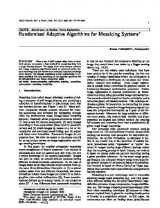
Fig. 1.
IEEE TRANSACTIONS ON NEURAL NETWORKS, VOL. 11, NO. 2, MARCH 2000
Convergence of the first four principal eigenvectors of A by the gradient descent (22) and steepest descent (26) algorithms for stationary data.
greater than zero, will eventually reach a global minimum . of The convergence of algorithm (22) can now be established by referring to Theorem 1 of Ljung [4], [13]. Theorem 4: Let A1–A3 hold. Assume that with probability visits infinitely often a compact subset one the process of the domain of attraction of one of the asymptotically stable . Then, with probability points one
stationary Gaussian data, and the second set on nonstationary Gaussian data. We then compared the steepest descent algorithm against state-of-the-art adaptive PCA algorithms. A. Experiments with Stationary Data We generated 500 samples of ten-dimensional Gaussian data with mean zero and covariance given below. Note that this covariance matrix is obtained from the first covariance matrix in [19] multiplied by two. The covariance matrix is shown in (37a) at the bottom of the next page. The eigenvalues of the covariance matrix are
Proof: By Theorem 2, are asymptotically stable points of the ODE (37). Since we assume visits a compact subset of the domain of attraction of that infinitely often, Lemma 1 then implies the theorem.
V. EXPERIMENTAL RESULTS We did two sets of experiments to test the performance of the new PCA algorithms. We did the first set of experiments on
Clearly, the first four eigenvalues are significant and we adaptively compute the corresponding eigenvectors. In order to com, we generated random data pute the online data sequence from the above covariance matrix. We generated vectors
CHATTERJEE et al.: ALGORITHMS FOR ACCELERATED CONVERGENCE OF ADAPTIVE PCA
Fig. 2.
345
Convergence of the first four principal eigenvectors of A by the gradient descent (22) and conjugate direction (29) algorithms for stationary data.
from by using algorithm (36) with . We compute the correlation matrix after collecting all 500 samples as
We refer to the eigenvectors and eigenvalues computed from this by a standard numerical analysis method [11] as the actual values. We used the adaptive gradient descent (22), steepest descent (26), conjugate direction (29), and Newton–Raphson (30) algo. We start all algorithms on the random data sequence
(37a)
346
Fig. 3.
IEEE TRANSACTIONS ON NEURAL NETWORKS, VOL. 11, NO. 2, MARCH 2000
Convergence of the first four principal eigenvectors of A by the gradient descent (22) and Newton–Raphson (30) algorithms for stationary data.
rithms with ONE, where ONE is an matrix whose all elements are ones. In order to measure the convergence and accuracy of the algorithms, we computed the direction cosine at th update of each adaptive algorithm as
Direction Cosine
(38)
is the estimated eigenvector of at th update, and where is the actual eigenvector computed from all collected samples by a conventional numerical analysis method. Figs. 1–4 show the iterates of the four algorithms to compute the first four principal eigenvectors of . For the gradient de. For the conscent (22) algorithm, we used jugate direction method, we used the Hestenes–Stiefel method to compute . For the steepest descent, conjugate direction, by solving a cubic and Newton–Raphson methods, we chose equation as described in Sections III-B–III-D, respectively. It is clear from Figs. 1–4, that the steepest descent, conjugate direction, and Newton–Raphson algorithms converge faster than
the gradient descent algorithm in spite of a careful selection of for the gradient descent algorithm. Besides, the new algorithms do not require ad hoc selections of . Instead, the gain and are computed from the online data separameters quence. Comparison between the four algorithms in Fig. 4, show small differences between them for the first four principal eigenvectors of . Among the three faster converging algorithms, the steepest descent algorithm (26) requires the smallest amount computation per iteration. Therefore, these limited experiments show that the steepest descent adaptive algorithm (26) is most suitable for optimum speed and computation among the four algorithms presented here. B. Experiments with Nonstationary Data In order to demonstrate the tracking ability of the algorithms with nonstationary data, we generated 500 samples of zero-mean ten-dimensional Gaussian data with the covariance matrix stated before. We then drastically changed the data sequence by generating 1000 samples of zero-mean ten-dimensional Gaussian data with the covariance matrix below (from
CHATTERJEE et al.: ALGORITHMS FOR ACCELERATED CONVERGENCE OF ADAPTIVE PCA
347
Fig. 4. Convergence of the first four principal eigenvectors of A by the gradient descent (22), steepest descent (26), conjugate direction (29), and Newton–Raphson (30) algorithms for stationary data.
[19]) as shown in (38a) at the bottom of the next page. The eigenvalues of this covariance matrix are
which are drastically different from the previous eigenvalues. from by using algorithm (36) with We generated . We used the adaptive gradient descent (22), steepest descent (26), conjugate direction (29), and Newton–Raphson , and (30) algorithms on the random observation sequence measured the convergence accuracy of the algorithms by computing the direction cosine at th update of each adaptive algorithm as shown in (38). We start all algorithms with ONE, where ONE is an matrix whose all elements are ones. Figs. 5–8 show the iterates of the four algorithms to compute the first four principal eigenvectors of the two covariance matrices described before. For the gradient descent (22) algorithm, . For the conjugate direction method, we used we used the Hestenes–Stiefel method to compute . For the
steepest descent, conjugate direction and Newton–Raphson methods, we chose by solving a cubic equation as described in Sections III-B–III-D, respectively. Once again, it is clear from Figs. 5–8, that the steepest descent, conjugate direction, and Newton–Raphson algorithms converge faster and track the changes in data much better than the traditional gradient descent algorithm. In some cases, such as Fig. 6 for the third principal eigenvector, the gradient descent algorithm fails as the data sequence changes, but the new algorithms perform correctly. Comparison between the four algorithms in Fig. 8, show small differences between them for the first four principal eigenvectors. Once again, among the three faster converging algorithms, since the steepest descent algorithm (26) requires the smallest amount computation per iteration, it is most suitable for optimum speed and computation. C. Comparison with State-of-the-Art Algorithms We compared our steepest descent algorithm (26) with Yang’s projection approximation subspace tracking (PASTd) algorithm [23], Bannour and Sadjadi’s RLS algorithm [3], and
348
IEEE TRANSACTIONS ON NEURAL NETWORKS, VOL. 11, NO. 2, MARCH 2000
Fig. 5. Convergence of the first four principal eigenvectors of two covariance matrices by the gradient descent (22) and steepest descent (26) algorithms for nonstationary data.
Fu and Dowling’s CGET1 algorithm [9], [10]. We first tested the four algorithms on the stationary data described in Section V-A. ( ) matrix whose all elements We define ONE as an are ones. The initial values for each algorithm are as follows:
Our steepest descent algorithm ONE
(38a)
CHATTERJEE et al.: ALGORITHMS FOR ACCELERATED CONVERGENCE OF ADAPTIVE PCA
349
Fig. 6. Convergence of the first four principal eigenvectors of two covariance matrices by the gradient descent (22) and conjugate direction (29) algorithms for nonstationary data.
Yang’s projection approximation subspace tracking (PASTd) algorithm ONE and
for
Bannour and Sadjadi’s RLS algorithm ONE and
ONE
Fu and Dowling’s conjugate gradient eigenstructure tracking (CGET1) algorithm
We next applied the four algorithms on nonstationary data described in Section V-B with in (36). The results of this experiment are shown in Fig. 10. We observe that the steepest descent and CGET1 algorithms perform quite well for all four principal eigenvectors. The PASTd algorithm performs better than the RLS algorithm in handling nonstationarity. This is expected since the PASTd algorithm accounts for nonstationarity with a forgetting factor , whereas the RLS algorithm has no such option. of
ONE and We found that the performance of the PASTd and RLS algoand rithms depended considerably on the initial choices of , respectively. We, therefore, chose the initial values that gave us the best results for most experiments. The results of this experiment are shown in Fig. 9. We observe, from Fig. 9 that the steepest descent and CGET1 algorithms perform quite well for all four principal eigenvectors. The RLS performed a little better than the PASTd algorithm for the minor eigenvectors. For the major eigenvectors, all algorithms performed well. The differences between the algorithms were evident for the minor (third and fourth) eigenvectors.
VI. CONCLUDING REMARKS We present an unconstrained objective function to obtain various new adaptive algorithms for PCA by using nonlinear optimization methods such as gradient descent (GD), steepest descent (SD), conjugate gradient (CG), and NR. We analyze the landscape of the unconstrained cost function. Convergence analysis of the GD adaptive algorithm is also presented. Comparison among these algorithms with stationary and nonstationary data show that the SD, CG, and NR algorithms have faster tracking abilities compared to the GD algorithm.
350
IEEE TRANSACTIONS ON NEURAL NETWORKS, VOL. 11, NO. 2, MARCH 2000
Fig. 7. Convergence of the first four principal eigenvectors of two covariance matrices by the gradient descent (22) and Newton–Raphson (30) algorithms for nonstationary data.
Further consideration should be given to the computational complexity of the algorithms. SD, CG, and NR algorithms have . If, however, we use the computational complexity of instead of (36) in the GD algorithm, estimate , although then the computational complexity drops to the convergence gets slower. The CGET1 algorithm has com. The PASTd and RLS algorithms have complexity . However, their convergence is slower than the plexity SD and CGET1 algorithms as shown in Figs. 9 and 10. Further note that our GD algorithm can be implemented by parallel architecture as shown by the examples in [8].
We have tr (A.2) where
APPENDIX A. Computation of
in (12), we compute
From
Simplifying (A.2), we obtain the cubic equation below
for Steepest Descent that minimizes
, where
where ; ; ; (A.1) Here
is the Hessian of
given in (25).
CHATTERJEE et al.: ALGORITHMS FOR ACCELERATED CONVERGENCE OF ADAPTIVE PCA
351
Fig. 8. Convergence of the first four principal eigenvectors of two covariance matrices by the gradient descent (22), steepest descent (26), conjugate direction (29), and Newton–Raphson (30) algorithms for nonstationary data.
It is well known that a cubic polynomial has at least one real root. The roots can also be computed in closed form as shown in terms of , we obtain in [1]. Expressing
If a root is complex, then and are complex, and clearly, this is not the root we are looking for. If we have three real roots, then we can either take the root corresponding to or the one corresponding to minimum .
rium points of the diagonal elements of the Jacobian described in (A.3). We prove the theorem by induction. From in (12) we have
We expand vectors of as
(A.4) in terms of the entire orthonormal set of eigen-
(A.5) Substituting this
B. Proof of Theorem 1 In order to satisfy the first-order conditions for the existence of the equilibrium points of the joint objective for , we need to find a functions such that for (A.3) , for which the We define a matrix columns are the weight vectors that converge to the principal eigenvectors of , respectively. We first find the equilib-
into (A.4), and multiplying it to the left by , and then equating it to zero, we get (A.6)
for
, which gives us (A.7)
or (A.8)
352
IEEE TRANSACTIONS ON NEURAL NETWORKS, VOL. 11, NO. 2, MARCH 2000
Fig. 9. Convergence of the first four principal eigenvectors of A by our steepest descent (26), Yang’s PASTd, Bannour–Sadjadi’s RLS, and Fu–Dowling’s CGET1 algorithms for stationary data.
for
By substituting it to the left by
. Rewriting (A.8), we obtain
into (A.10), and multiplying , and then equating it to zero, we get
(A.9) Since is positive definite and since each eigenvalue of is of for , unit multiplicity, from (A.9) we obtain , and for . Clearly, there can be . Thus, the equilibrium points of at most one nonzero are
(A.11) . Here is the Kronecker’s delta. We have for the following two conditions: , then we obtain from (A.11) 1) If (A.12) or (A.13)
where
is a permutation of the eigenvectors , , or . We next consider the equilibrium points of is gradient with respect to
, and , whose
(A.10)
, then we obtain from (A.13) that all If for . On the other hand, if then we obtain an equation that is similar to (A.8). We conclude and all other . that , then we obtain an equation that is same as 2) If , or there is at (A.6), from which we conclude that . most one nonzero are Thus, the equilibrium points of (A.14)
CHATTERJEE et al.: ALGORITHMS FOR ACCELERATED CONVERGENCE OF ADAPTIVE PCA
353
Fig. 10. Convergence of the first four principal eigenvectors of two covariance matrices by our steepest descent (26), Yang’s PASTd, Bannour–Sadjadi’s RLS, and Fu–Dowling’s CGET1 algorithms for nonstationary data.
where ,
is a permutation of the eigenvectors , or . Furthermore, if , then
. We now assume that the equilibrium points of where then of
, and can be are (A.15) , and
is a permutation of the eigenvectors , , or . Furthermore, for any , if can be . We now consider the equilibrium points , whose gradient with respect to is
(A.16) By substituting it to the left by
for two conditions.
into (A.16), and multiplying , and then equating it to zero, we get
and
(A.17) . We have the following
1) If (A.17)
for
, then we obtain from (A.18)
or (A.19) , then we obtain from (A.19) that all If for . On the other hand, if then we obtain an equation that is similar to (A.8). We conclude and all other . that at most one for , then we obtain an 2) If equation that is same as (A.6), from which we conclude , or there is at most one nonzero . that are Thus, the equilibrium points of (A.20) is a permutation of the eigenvectors where , and , , or . Furthermore, for , if , then can be . any We can now check that these critical points also satisfy the remaining first order conditions given in (A.3). Be-
354
IEEE TRANSACTIONS ON NEURAL NETWORKS, VOL. 11, NO. 2, MARCH 2000
sides, equating the remaining terms of (A.3) to zero, does not yield any new stationary point. Thus, all the equilibfor rium points of the joint objective functions are (A.21) where are the
,
, or
for is an indefinite matrix. Thus, is , whereas a stable equilibrium point of the energy function for are unstable equilibrium points of . for We next assume that are stable equilibrium points for the energy . Then, for , we have from (A.23) function
, and .
permutations of
C. Proof of Theorem 2 in (12), we define the
From the objective function following energy functions:
The are (
(A.22) ,(
for
) Let us assume that
eigenvectors of . The eigenvalues are for ), for , and for ( ). Thus, is positive definite. On the ( ), then other hand, if
for some
; i.e.,
The are
Next, we perturb the th column of
by
. We observe that
Clearly, the energy function decreases for some . for some , We next prove that if are unstable equilibrium points of then the critical points with respect to as (A.22). We obtain the Hessian of
(A.23)
eigenvalues
of for
, and
for ( ). Thus, is an indefinite matrix. for We, therefore, see that are the stable equilibrium points of . From the above analysis, we conclude that are stable equilibrium points of the energy functions (A.22), whereas, , where or for are unstable equilibrium points. D. Proof of Theorem 3 Regarding algorithm (21), for simplicity of notation, we use instead of for this proof
(A.24) be the first principal eigenvector of corresponding to Let . By multiplying (A.24) the largest eigenvalue , we obtain on the left by (A.25)
We prove the result by induction. We note that where The eigenvectors of are . The eigenfor , and for ( ). Clearly, values are is positive definite. On the other hand, we observe that
Thus, if
. From (A.25),
, then
if
if
for The eigenvectors of values are
are for
, and
for
(
(A.26) . The eigen). Clearly,
Due to assumption A2, a uniform upper bound for
exists.
CHATTERJEE et al.: ALGORITHMS FOR ACCELERATED CONVERGENCE OF ADAPTIVE PCA
REFERENCES [1] M. Artin, Algebra. Englewood Cliffs, NJ: Prentice-Hall, 1991. [2] P. Baldi and K. Hornik, “Learning in linear neural networks: A survey,” IEEE Trans. Neural Networks, vol. 6, pp. 837–857, 1995. [3] S. Bannour and M. R. Azimi-Sadjadi, “Principal component extraction using recursive least squares learning,” IEEE Trans. Neural Networks, vol. 6, pp. 457–469, 1995. [4] A. Benveniste, A. Metivier, and P. Priouret, Adaptive Algorithms and Stochastic Approximations. New York: Springer-Verlag, 1990. [5] C. Chatterjee, V. P. Roychowdhury, and E. K. P. Chong, “On relative convergence properties of principal component analysis algorithms,” IEEE Trans. Neural Networks, vol. 9, pp. 319–329, March 1998. [6] C. Chatterjee, V. P. Roychowdhury, M. D. Zoltowski, and J. Ramos, “Self-organizing and adaptive algorithms for generalized eigendecomposition,” IEEE Trans. Neural Networks, vol. 8, pp. 1518–1530, November 1997. [7] Y. Chauvin, “Principal component analysis by gradient descent on a constrained linear Hebbian cell,” in Proc. Joint Int. Conf. Neural Networks, vol. I, San Diego, CA, 1989, pp. 373–380. [8] A. Cichocki and R. Unbehauen, Neural Networks for Optimization and Signal Processing. New York: Wiley, 1993. [9] Z. Fu and E. M. Dowling, “Conjugate gradient eigenstructure tracking for adaptive spectral estimation,” IEEE Trans. Signal Processing, vol. 43, pp. 1151–1160, 1995. , “Conjugate gradient projection subspace tracking,” in Proc. 1994 [10] Conf. Signals, Syst. Comput., vol. 1, Pacific Grove, CA, 1994, pp. 612–618. [11] G. H. Golub and C. F. VanLoan, Matrix Computations. Baltimore, MD: Johns Hopkins Univ. Press, 1983. [12] S. Haykin, Neural Networks—A Comprehensive Foundation. New York: Macmillan, 1994. [13] L. Ljung, “Analysis of recursive stochastic algorithms,” IEEE Trans. Automat. Contr., vol. AC-22, no. 4, pp. 551–575, August 1977. [14] D. Luenberger, Linear and Nonlinear Programming. Reading, MA: Addison-Wesley, 1984. [15] G. Mathew, V. U. Reddy, and S. Dasgupta, “Adaptive estimation of eigensubspace,” IEEE Trans. Signal Processing, vol. 43, pp. 401–411, 1995. [16] Y. Miao and Y. Hua, “Fast subspace tracking and neural-network learning by a novel information criterion,” IEEE Trans. Signal Processing, vol. 46, pp. 1967–1979, 1998. [17] E. Oja and J. Karhunen, “On stochastic approximation of the eigenvectors and eigenvalues of the expectation of a random matrix,” J. Math. Anal. Applicat., vol. 106, pp. 69–84, 1985. [18] M. Plumbley, “Lyapunov function for convergence of principal component algorithms,” Neural Networks, vol. 8, pp. 11–23, 1995. [19] T. Okada and S. Tomita, “An optimal orthonormal system for discriminant analysis,” Pattern Recognition, vol. 18, no. 2, pp. 139–144, 1985. [20] T. D. Sanger, “Optimal unsupervised learning in a single-layer linear feedforward neural network,” Neural Networks, vol. 2, pp. 459–473, 1989. [21] T. K. Sarkar and X. Yang, “Application of the conjugate gradient and steepest descent for computing the eigenvalues of an operator,” Signal Processing, vol. 17, pp. 31–38, 1989. [22] L. Xu, “Least mean square error reconstruction principle for self-organizing neural-nets,” Neural Networks, vol. 6, pp. 627–648, 1993. [23] B. Yang, “Projection approximation subspace tracking,” IEEE Trans. Signal Processing, vol. 43, no. 1, pp. 95–107, 1995. [24] X. Yang, T. K. Sarkar, and E. Arvas, “A survey of conjugate gradient algorithms for solution of extreme eigen-problems of a symmetric matrix,” IEEE Trans. Acoust., Speech, Signal Processing, vol. 37, pp. 1550–1556, 1989.
355
[25] W. Zhu and Y. Yang, “Regularized total least squares reconstruction for optical tomographic imaging using conjugate gradient method,” in Proc. Int. Conf. Image Processing, vol. 1, Santa Barbara, CA, 1997, pp. 192–195.
Chanchal Chatterjee (M’88) received the B.Tech. degree in electrical engineering from the Indian Institute of Technology, Kanpur, India, and the M.S.E.E. degree from Purdue University, West Lafayette, IN, in 1983 and 1984, respectively. In 1996, he received the Ph.D. degree in electrical and computer engineering from Purdue University. Between 1985 and 1995, he worked at Machine Vision International and Medar Inc., both in Detroit, MI. He is currently a Senior Algorithms Specialist at BAE Systems, San Diego, CA. He is also affiliated with the Electrical Engineering Department at the University of California, Los Angeles. His areas of interest include image processing, computer vision, neural networks, and adaptive algorithms and systems for pattern recognition and signal processing.
Zhengjiu Kang (M’98) received the B.S. degree in control engineering from Harbin Shipbuilding Engineering Institute, China, in 1991, and the Ph.D. degree in system engineering from Xi’an Jiaotong University, China, in 1996. He is now working toward the Ph.D. degree in wireless communications. From 1996 to 1997, he was a Researcher at Control Information Systems Lab, Seoul National University, Korea. Since 1997, he has been with the Electrical Engineering Department at University of California, Los Angeles. His current research interests include adaptive algorithms, wireless communications, neural networks, and parallel processing.
Vwani P. Roychowdhury received the B. Tech. degree from the Indian Institute of Technology, Kanpur, India, and the Ph.D. degree from Stanford University, Stanford, CA, in 1982 and 1989, respectively, all in electrical engineering. From August 1991 until June 1996, he was a Faculty Member at the School of Electrical and Computer Engineering at Purdue University. He is currently a Professor in the Department of Electrical Engineering at the University of California, Los Angeles. His research interests include parallel algorithms and architectures, design and analysis of neural networks, application of computational principles to nanoelectronics, special purpose computing arrays, VLSI design, and fault-tolerant computation. He has coauthored several books, including Discrete Neural Computation: A Theoretical Foundation (Englewood Cliffs, NJ: Prentice-Hall, 1995) and Theoretical Advances in Neural Computation and Learning (Boston, MA: Kluwer, 1994).