Algorithms for Querying by Spatial Structure Dimitris Papadias1, Nikos Mamoulis1 and Vasilis Delis2 1
Department of Computer Science Hong Kong University of Science and Technology Clear Water Bay, Hong Kong {dimitris, mamoulis}@cs.ust.hk Abstract: Structural queries constitute a special form of content-based retrieval where the user specifies a set of spatial constraints among query variables and asks for all configurations of actual objects that (totally or partially) match these constraints. Processing such queries can be thought of as a general form of spatial joins, i.e., instead of pairs, the result consists of n-tuples of objects, where n is the number of query variables. In this paper we describe a flexible framework which permits the representation of configurations in different resolution levels and supports the automatic derivation of similarity measures. We subsequently propose three algorithms for structural query processing which integrate constraint satisfaction with spatial indexing (R-trees). For each algorithm we apply several optimization techniques and experimentally evaluate performance using real data.
1. Introduction Several types of spatial queries have been the focus of active research in the database community: window queries [G84], nearest neighbors [RKV95], relationbased queries [PTSE95] etc. The above types retrieve all objects in the database that satisfy some spatial property with respect to a fixed reference object or window. Recently the focus has shifted towards spatial joins [R91] [G93] [BKS93], which involve the retrieval of pairs of objects that satisfy some spatial predicate (most often overlap). This work examines an alternative form of spatial information processing, namely, queries involving the retrieval of n-tuples (n>2) of objects that satisfy some spatial structure. Structure is described as a set of spatial constraints between query variables which can be expressed either by a "verbal" (e.g., select X, Y, Z, from Roadmap, where overlaps(X,Y) and north(Y,Z)) or pictorial language (e.g., by drawing a prototype configuration on a sketch-board). This type of queries can be thought of as the generalization of spatial joins (if Permission to copy without fee all or part of this material is granted provided that the copies are not made or distributed for direct commercial advantage, the VLDB copyright notice and the title of the publication and its date appear, and notice is given that copying is by permission of the Very Large Data Base Endowment. To copy otherwise, or to republish, requires a fee and/or special permission from the Endowment. Proceedings of the 24th VLDB Conference, New York, USA, 1998
2
Computer Engineering and Informatics Department and Computer Technology Institute University of Patras, Greece
[email protected] the relation between variables is overlap, it corresponds to common multi-way spatial join). From a different perspective, structural queries constitute a special class of image similarity retrieval, where the query specifies an input configuration to be matched with stored images. Similarity is based on relative locations and not on visual characteristics (e.g., colour, shape). Let n be the query size (number of variables) and N be the data size (number of image objects): in the worst case (exhaustive search), all n-permutations of N objects have to be searched in order to find solutions (i.e., N!/(N-n)!). In real DBMSs where N>>n, this number is O(Nn), meaning that the retrieval of structural queries can be exponential to the query size. Query processing becomes more expensive if inexact matches are to be retrieved, a situation which arises very often in practical applications. In order to avoid this problem, most related previous techniques (e.g., [GR95] [NNS96]) have focused on a specific instance where images consist of known (labelled) objects and queries express spatial constraints among a subset of these objects. [PF97] employ R-trees to solve structural queries for images that contain a constant number of labelled objects (e.g., lungs) and a small number of unlabelled ones (e.g., tumours). Although their method is efficient for domains involving numerous small images with few unlabelled objects (e.g., medical databases of X-rays) it is not applicable to large images of unlabelled objects. In this paper we deal with the general problem where large images contain arbitrary numbers of unlabelled objects. In order to provide a general solution, we present a unified framework for structural similarity, which can represent various resolution levels and automates the derivation of similarity measures. We then propose algorithms that can solve the problem for considerable data and query sizes. These algorithms utilize ideas from related work in spatial databases (spatial join processing) and AI (constraint satisfaction algorithms). Although the problem of querying by structure is not a new one (it has been around since the early stages of computer vision [BB84]), to the best of our knowledge this is the first approach to provide a solution which combines search algorithms with spatial indexing and can be applied for secondary memory retrieval. Our
techniques have a wide range of potential applications in various areas (e.g., GIS, Multimedia Databases, VLSI). The rest of the paper is organized as follows: Section 2 describes a binary string encoding for the representation of structure in multiple resolutions and dimensions. Sections 3 outlines the problem and provides examples of spatial queries and their processing. Sections 4, 5 and 6 describe three algorithms for structural query processing: the first one extends traditional spatial join methods for R-trees to multi-way (nested) joins. The second algorithm uses a search heuristic to prune the windows where query variables can be instantiated from, while the third one combines ideas from the first two algorithms. Section 7 compares the performance of the algorithms under several conditions. Finally, Section 8 concludes with future research directions.
the variable's associated region ("0" corresponds to an empty intersection while "1" corresponds to a non-empty one). Thus, we can define 1D relations to be 9-tuples (Rrstuvwxyz : r, s, t, u, v, w, x, y, z ∈ {0,1}). Such a consecutive partitioning of space constitutes a resolution scheme. There are several possible schemes; the particular choice is affected by the users' expectations or the application's requirements, as every scheme can refine or generalize a particular relation class. For example, when distance relations are not needed we can apply a scheme with only five bits (two corresponding to the points of the reference interval) which defines the 13 relations between intervals proposed by Allen [A83]. The feasible relations at a particular resolution scheme are called primitive relations. In general, the less the binary variables, the coarser the resolution, and vice versa. If b is the number of bits used by the resolution scheme, the number of primitive relations in 1D is b(b+1)/2 - k, where k is the number of point variables, i.e. intervals of the form [a,a]. For b=9, k=4 we get 41 relations (see Figure 2), while for b=5, k=2, there exist 13 (Allen's) relations. Each spatial relation is mapped onto a set of primitive relations. For instance, left can be mapped onto {R100000000, R110000000, R111000000, R011000000, R001000000} and near onto {R001000000, R000000100}. Disjunction of spatial relations (e.g., left or near) are represented by the unions of the corresponding sets, and conjunctions by their intersection (e.g., {R001000000} corresponds to left-near). The next step is to provide a mechanism for representing similarities among relations independently of the resolution scheme. [F92] defined the concept of conceptual neighborhood as a cognitively plausible way to measure similarity among Allen's interval relations. A neighborhood is represented as a graph whose nodes denote relations that are linked through an edge, if they can be directly transformed to each other by continuous interval deformations. Depending on the allowed deformation (e.g., movement, enlargement), several graphs may be obtained.
2. A Framework for Structural Similarity We will initially confine our discussion to one dimension and address the most common types of relations proposed and mathematically defined so far in the spatial domain [PS94], namely topological (e.g., inside, overlaps), directional (e.g., north, northeast) and qualitative distance relations (e.g., near, far). Figure 1 illustrates the three types of 1D relations assuming that the lower interval is the reference object and the upper interval is the primary one. Our goal is to provide a unified and adjustable framework which permits the definition of any type of spatial relation and the automatic generation of similarities between them. Assume that in a particular application the only relations of interest are the ones in Figure 1, and we are given a (reference) interval [a,b]. Then we identify nine potential regions of interest: 1.(-∞,a-δ) 2.[a-δ,a-δ] 3.(a-δ,a) 4.[a,a] 5.(a,b) 6.[b,b] 7.(b, b+δ) 8.[b+δ, b+δ] 9.(b+δ,+∞) For each of the above regions we associate a binary variable, r, s, t, u, v, w, x, y, z, respectively (see Figure 2). Given a primary interval [c,d], the value of every variable indicates the result of the intersection between [c,d] and topological relations meets
overlaps
equal
covers
covered by
contains
contained by
disjoint
distance relations
directional relations
far
left /
/
left-near /
/
/
/
/
Figure 1 Categorization of 1D relations
/
/
R100000000
R110000000
δ
δ
R111000000
R111100000
δ
R111110000
R011100000
R011000000
R011110000
δ
δ
R001110000
δ
δ
δ
δ
R011111000
δ
R001100000
R001000000
R111111000
δ
δ
R000110000
δ
R001111000
δ
R000111000
R111111100
R011111100
δ
δ
R001111100
δ
δ
R000111100
δ
R000010000
R000011000
R000011100
δ
bit:
0 1 2 3 r s t u
-∞
δ
4 v
a
5 6 7 8 w x y z
b
δ
R111111111
R111111110
δ
δ
R000001100
δ
δ
δ
δ
R011111110
δ
δ
R001111110
δ
δ
R000111110
δ
R011111111
δ
δ
R001111111
δ
δ
R000111111
δ
δ
R000011110
R000011111
δ
δ
R000001110
R000001111
δ
δ
R000000110
R000000111
∞ R000000100
δ
δ
δ
R000000011
δ
R000000001
δ
Figure 2 1D Conceptual neighborhood including distances
Figure 2 represents the neighborhood graph for a distance-enhanced resolution scheme, assuming that a minimal deformation is a movement of a single interval endpoint. Starting from relation R100000000 and extending the upper interval to the right, we derive relation R110000000. With a similar extension we can get the transition from R110000000 to R111000000 and so on. R100000000 and R111000000 are called 1st degree neighbors of R110000000. The distance d between two relations is equal to the length of the shortest path connecting them in the neighborhood graph. The binary string representation enables automatic calculation of distances using the pseudo-code of Figure 3, which counts the minimal number of “0”s that have to be replaced with "1"s in order to make the two strings identical. For example d(R000110000, R010000000) = 5 and d(R000110000, R110000000) = 6 (the underlined 0s are the ones counted during the calculation of distance). The distance between a relation R and a relation set {R1,…,Ri} equals the minimum distance between R and any of R1,…,Ri (e.g., d(R000110000, {R010000000, R110000000})= 5). INT distance(relation R1, relation R2) R = R1 OR R2; /*bitwise OR */ d = 0; FOR i:= R.leftmost_1 to R.rightmost_1 DO IF R1[i]=0 THEN d ++; IF R2[i]=0 THEN d ++; RETURN (d);
Figure 3 Distance calculation
The encoding and distance calculation can be extended accordingly to multi-dimensional spaces. A Ddimensional relation is defined as a D-tuple of 1D projections, e.g. R110000000-111000000 = (R110000000, R111000000). In order to derive a neighboring relation we have to replace one of the constituent 1D projections with its neighbors. As a result, computing D-relation distances is reduced to the already solved problem of computing 1D distances. In this paper we calculate the distance between two multi-dimensional relations by summing up the distances in each dimension (other metrics, such as Euclidean [NNS96], can also be applied). The advantages of the proposed framework are i) the expressiveness of the encoding in the sense that given a binary string, the corresponding spatial configuration can be easily inferred, and vice versa, ii) efficient automatic calculation of neighborhoods and relation distance, and iii) the uniform representation of all three types of relations (topological, directional, distance) in various resolution levels. For the sake of clarity, in the rest of the paper we use the distance enhanced resolution scheme of Figure 2. However for more realistic applications, sufficiently fine schemes (large encoding strings) can be used, while retaining the model's properties. The algorithms of the following sections are independent of the resolution and can be applied with any set of spatiotemporal relations. For a number of alternative resolution schemes and a more detailed description of the framework see [DPM98].
(a) Query
(b) Constraints
(c) Solution
Figure 4 Example query
3. Structural Queries The projection-based definitions of relations and similarity measures of Section 2 are particularly suitable for structural similarity retrieval, because spatial databases often utilize minimum bounding rectangles (i.e., projection-based approximations) as a fast filter step to exclude the objects that could not possibly satisfy a query [O86]. Furthermore, structural queries do not always have exact matches and crisp results. Rather, the output should have an associated "score" to indicate its similarity to the query. By adoption, this score is inversely proportional to the degree of neighborhood. A structural query can be formalised as a binary constraint satisfaction problem [N89] (CSP) which consists of: • A set of n variables, V0,V1,…,Vn-1 that appear in the query. • For each variable Vi a finite domain Di ={u0,…, uN-1} of N potential values which correspond to image objects. In this paper we assume that all domains are identical, i.e., each variable can be instantiated to any image object. • For each pair of variables Vi,Vj a binary spatial constraint Cij which is a set of primitive relations. Consider, for example, the query of Figure 4(a) which is a spatial arrangement of n=4 variables, expressed using a query-by-sketch language. Assuming the distanceenhanced resolution scheme of Figure 2, the set of query constraints between all variable pairs is illustrated in Figure 4(b). The domain of each variable is the set of objects in the image to be searched. Figure 4(c) illustrates a solution where variable V0 is instantiated to object 143, V1 to object 207 and so on. Although the particular language specifies relations between all pairs of variables, in some cases (e.g., verbal languages), queries may be incomplete (some Cij may be left unspecified) or
indefinite (Cij may be disjunctions of relations). A binary instantiation {Vi←uk, Vj←ul} is consistent, if R(uk,ul) ⊆ Cij. For instance, the constraint between V0 and V3 is R100000000-111000000, which is also the relation between their corresponding instantiations (143,42) in Figure 4(c); therefore, {V0←143, V3←42} is consistent. We define the binary degree of inconsistency τ of {Vi← uk, Vj ←ul} as the distance between Cij and R(uk,ul). Although the constraint between V0 and V1 is R001111000001111100, the relation between objects 143 and 207 is R001111000-001111000; hence, τ =1 for {V0←143, V1←207}. The degree of inconsistency T of a solution {V0← up, …, Vn-1 ← ur} is the sum of all binary inconsistency degrees: T= d (Cij, R(uk , ul )) where {Vi ← uk, Vj ← ul}
∑
∀ij, 0≤i , j< n
Degrees of inconsistency are used for the retrieval of configurations that match the input structure closely, but not perfectly. The maximum allowed T and τ are submitted with a query in order to adjust the trade-off between the level of approximation and the cost of query processing. For instance, if T=6 and τ=2, only solutions that produce total relation difference ≤ 6 and pair-wise difference ≤ 2 will be retrieved. Obviously as T and τ increase, so does the number of solutions, but also the cost of query processing. 3.1 Forward Checking with Dynamic Value Ordering A number of algorithms have been proposed for solving CSPs [N89]. One of the most effective, is forward checking (FC) [HE80] [BG95] which has been shown to outperform the rest for a wide range of problems involving "crisp" constraints [BvR95]. FC must be modified for structural queries in order to handle soft constraint processing using T and τ.
The adjusted version works as follows: when a variable Vi is assigned a value uk, the domain of each future (un-instantiated) variable Vj is pruned according to uk and the constraint Cij, for all j>i. That is, all values ul that produce a distance d(Cij,R(uk,ul))>τ are removed from the domain of Vj. The same happens for values that produce global inconsistency degree > T, taking into account the constraints between Vj and all instantiated variables1. Consequently, when we reach instantiation level i (variables up to Vi have been instantiated), the values of variables V0,…,Vi will constitute a partial solution, and the domains of future variables will contain only values that may lead to a (complete) solution given the instantiations so far. The procedure of pruning the domains of the future variables is called check forward. If, after a check forward the whole domain of a future variable is eliminated, the algorithm un-assigns the current variable’s value, and restores the values of future variables, which were eliminated due to the current instantiation. When the domain of the current variable is exhausted the algorithm backtracks to the previous one and assigns a new value to it. FC outputs a solution whenever the last variable is given a value, and terminates when it backtracks from the first variable. In order to keep track of the allowable values for each variable at every instantiation level, FC uses a nxnxN domain table. Each element of domain[i][j] is an array of N values that Vj can take at different levels. Before FC starts, domain[0][j] is initialized to D for all variables. When V0 is assigned a value up, domain[1][j] is computed for each remaining Vj, by including only values ul ∈ domain[0][j] such that d(C0j,R(up,ul))≤τ. In general if uk is the current value of Vi, domain[i+1][j] is the subset of domain[i][j] which is valid w.r.t. Cij and uk. In this way, at each instantiation level the domain[i][j] of Vj continuously shrinks; when we reach level j, Vj gets instantiated from domain[j][j] which contains only values compatible with the instantiations of previous variables. If a value of Vi results in the domain of some Vj to become empty, a new value is chosen and domain[i+1][j] is re-initialized to domain[i][j]. Dynamic Variable Ordering (DVO) [BvR95] is a technique employed by several CSP algorithms to improve efficiency. The key idea behind FC-DVO is to reorder the future variables according to their domain size after “checking forward” at the current instantiation level. The variable with the minimum domain size becomes the next variable to be tested. In this way the number of search paths is minimized, because the variable with the smallest domain is the most likely to be 1
The inverse constraints Cji are also considered but, for the sake of simplicity, we omit these tests in the rest of the paper.
FC-DVO(Query q, int τ,T ) FOR j = 0 TO n-1 DO domain[0,j] = D /*initialize all domains to D */ i = 0; /* index to the current variable */ WHILE (TRUE) { new_value := chooseNextValue(domain[i][i]); IF new_value = NULL THEN /* end of domain */ IF i=0 THEN RETURN; ELSE i:=i-1; CONTINUE; /*Backtrack*/ ELSE instantiations[i] := new_value; /*store instantiation*/ IF i = n-1 THEN /*last variable instantiated*/ output_solution(instantiations); ELSE /* intermediate variable instantiated */ IF check_forward(i) THEN /* successful instantiation*/ DVO(i+1,n-1); /*var. with the smallest domain as next*/ i := i+1; /* successful instantiation: go forward */ } BOOLEAN check_forward(int i) FOR j = i+1 TO n-1 DO /*for all uninstantiated variables*/ domain[i+1][j]= domain[i][j]; FOR all values ul ∈ domain[i+1][j] IF d(Cij,R(instantiations[i],ul)) > τ OR T exceeded THEN domain[i+1][j]= domain[i+1][j]-{ul}; IF domain[i+1][j]=∅ THEN RETURN FALSE; RETURN TRUE;
Figure 5 Soft forward checking with dynamic value ordering
pruned out; the algorithm will backtrack faster in the case that there is no valid assignment after the current partial solution. DVO is responsible for changing the order of V1 and V2 in Figure 4(c). The pseudo-code of a non-recursive version of FC with DVO which can be applied for structural query processing is given in Figure 5. FC-DVO has two drawbacks for the current application. First it is inapplicable for large spatial databases, because the 3D domain table cannot fit in main memory. The second drawback is the fact that it does not utilize the existing spatial indices which may exist for spatial relations. The incorporation of R-trees [G84] and appropriate query processing techniques can solve both these problems. 3.2 Multi-Relation Spatial Join Structural queries can be viewed as multi-way spatial self-joins, where structural constraints correspond to join predicates. For example, a pair-wise spatial join is equivalent to a structural query with two variables related by a spatial constraint. The most influential technique for efficiently computing pair-wise, intersection joins using R-trees is presented in [BKS93]. It is based on the enclosure property: if two intermediate R-tree nodes do not intersect, there can be no MBRs below them that intersect. The algorithm first joins the high level nodes and then follows the links in order to find qualifying pairs below them (Figure 6).
SpatialJoin(Rtree_Node N[i], N[j]) FOR all Nl ∈ N[j] DO FOR all Nk ∈ N[i] with Nk ∩ Nl ≠ ∅ DO IF N[i] is a leaf page THEN output (Nk, Nl) ELSE ReadPage(Nk.ref); ReadPage(Nl.ref); SpatialJoin(N[k], N[l])
Figure 6 R-tree SpatialJoin
In the pseudo-code of Figure 6, as well as in the rest of the paper, we make the distinction between an R-tree node N[i] and its entries Nk, which correspond to MBRs included in N[i]. Nk.ref points to the corresponding node N[k] at the next (lower) level. Although SpatialJoin assumes that the nodes to be joined are of equal height, the extension to different heights is straightforward. Two local optimization techniques are used to improve the CPU speed of the above algorithm. The first, search space restriction, reduces the quadratic number of pairs to be evaluated when two nodes N[i], N[j] are joined. If an entry Nk ∈ N[i] does not intersect the MBR of N[j] (that is the MBR of all entries contained in N[j]), then there can be no entry Nl ∈ N[j], such that Nk and Nl overlap. Using this observation, space restriction performs two linear scans in the entries of both nodes before starting the SpatialJoin procedure, and prunes out from each node the entries that do not intersect the MBR of the other node. The second technique, based on the plane sweep paradigm [PS88], applies sorting in one dimension in order to reduce the computation time of the overlapping pairs between the nodes to be joined. In addition, [BKS93] apply a technique that uses pinning (or page fixing), a well known I/O buffer management method, to force page fetching according to the optimal order. In [HJR97], SpatialJoin was extended by introducing an on-the-fly indexing mechanism to optimize the execution order of matchings at intermediate levels. [BKSS94] study the multi-step processing of spatial joins using several approximations, while [BKS96] employ parallel execution. In order to use an arbitrary relation as the join condition in SpatialJoin, we need a mapping from relations, to bounding conditions between intermediate node entries that should be recursively joined. Table 1 shows the bounding condition BCij for Ni given Nj. This condition is based solely on the positions of the leftmost and rightmost 1's in Cij. In particular, the leftmost 1, determines the position of Ni.l with respect to Nj.u, while the rightmost 1 of Ni.u with respect to Nj.l (l and u represent the lower and upper node-MBR points respectively). Entries that do not satisfy these conditions can be excluded during search.
Ni.l < Nj.u - δ Ni.l ≤ Nj.u - δ Ni.l < Nj.u Ni.l ≤ Nj.u Ni.l ≤ Nj.u Ni.l ≤ Nj.u Ni.l < Nj.u + δ Ni.l ≤ Nj.u + δ Ni.l unlimited
R1XXXXXXXX R 01XXXXXXX R001XXXXXX R0001XXXXX R00001XXXX R000001XXX R 0000001XX R00000001X R000000001
RXXXXXXXX1 RXXXXXXX10 RXXXXXX100 RXXXXX1000 RXXXX10000 RXXX100000 RXX1000000 RX10000000 R100000000
(a) leftmost bit
Ni.u > Nj.l + δ Ni.u ≥ Nj.l + δ Ni.u > Nj.l Ni.u ≥ Nj.l Ni.u ≥ Nj.l Ni.u ≥ Nj.l Ni.u > Nj.l - δ Ni.u ≥ Nj.l - δ Ni.u unlimited
(a) rightmost bit
Table 1 Bounding condition BCij for Ni
Assume, for instance, the query "find all pairs (V2, V3) related by R000000001-001100000". An entry N2 is bounded with respect to N3 by the following conditions: (N2.u > N3.l + δ) on the x dimension, and by (N2.l < N3.u), (N2.u ≥ N3.l) on the y dimension. Figure 4.3 illustrates an example for axis x: if N3 is the intermediate node entry containing an object assigned to V3, then the upper point of candidate entries for N2 (N2.u) should lie in the grey area. Entries, like N'2, not satisfying this constraint, cannot contain consistent instantiations of V2. For approximate retrieval, bounding conditions are adapted to include τ. N'2 V3
N2
V2
δ
δ
N3
bounding condition for N 2 .u
Figure 7 Example of bounding condition for intermediate nodes
Using the above transformation, SpatialJoin is extended to handle multiple relations. Figure 8 illustrates the code for multi-relation spatial join (MJS). In this case, the desired relation Cij, as well as τ, are passed as parameters. Each BCij is computed using Cij, τ and Table 1 (inverse conditions are also computed, but omitted for clarity). Leaf nodes constitute solutions, if they are related by a relation whose distance from Cij is ≤ τ. Intermediate nodes are recursively searched if they satisfy BCij. MSJ(Rtree_Node N[i], N[j], RelationSet Cij, int τ) BCij = computeNodeBC(Cij,τ); FOR all Nl ∈ N[j] DO FOR all Nk ∈ N[i] DO IF N[i] is a leaf page THEN IF d(Cij,R(Nk, Nl)) ≤ τ THEN output (Nk, Nk, d) ELSE IF BCij(Nk, Nl) THEN ReadPage(Nk.ref); ReadPage(Nl.ref); MSJ(N[k], N[l], Cij, τ)
Figure 8 Multi-relation spatial join
Structural queries could be processed by executing MSJ for all pairs of variables and combining the binary solutions. The main problem with this approach is the
large number of pair-wise joins (six for the query of Figure 4) and the complexity of combining their results (which may be too large to fit in main memory). In the rest of the paper we propose three algorithms that avoid calculating intermediate results by incorporating ideas from forward checking and traditional spatial join processing.
4. A Multilevel Forward Checking Algorithm The first algorithm, multilevel forward checking (MFC), extends MSJ to deal with n-tuples instead of pairs. MFC finds all n-combinations of intermediate nodes (at each level of the R-tree) that may contain some solution objects and follows the references to the next level, until it reaches the leaves, where it outputs solutions. As an example consider the rectangles of Figure 9(a) which are organized in the R-tree of Figure 9(b) assuming a bucket size equal to three. The path to solution (d,e,a,k) of the example query is: (1,1,1,2) at the top, (B,B,A,D) at level 1 and (d,e,a,k) at level 0. 2 g d
B
e
C
i
c f
A
1
D k
b
a
j
l δ
(a) Image 1
level 2
level 1
level 0
A
a
b
f
2
B
c
d
e
l
k
j
D
C
g
i
(a) R-tree
Figure 9 Image and corresponding R-tree
The calculation of combinations of the qualifying nodes at each level (e.g., (1,1,1,1), (1,1,1,2), …., (2,2,2,2) for the top) is expensive, as their number can be as high as Cn, where C is the capacity of an R-tree bucket. Although the search space is not prohibitively large (usually n≤10 and C≤200), the computational burden is due to numerous appearances of the problem during query processing. Finding the subset of node combinations which is consistent with the input query can be treated as a local CSP at each level. In particular the problem consists of: • A set of n variables, V0,V1,…,Vn-1. • For each variable Vi a domain Di={N0,…,NI-1} of I (I≤ C) potential values which correspond to entries in Rtree node N[i].
• For each pair of variables Vi,Vj a binary constraint which: i] for intermediate nodes is a bounding condition BCij derived from Table 1 using the corresponding Cij and τ, ii] for leaf nodes is a constraint Cij (disjunction of primitive relations). The CSP in the case of the top level of the tree in Figure 9 has four variables V0,V1,V2,V3, which can be instantiated to entries 1 or 2 of the root. As we saw in the example of Figure 7, BC23 is: (N2.u > N3.l + δ) on the x dimension, and (N2.l < N3.u ) ∧ (N2.u ≥ N3.l) on the y dimension. The binary instantiation {V2←2, V3←1} cannot lead to a solution at the lower levels because (1.u < 2.l + δ). Therefore, all combinations (x,x,2,1) can be pruned out during search. MFC (Figure 10) applies forward checking to solve the CSP at each R-tree level: every time a variable Vi is instantiated to an entry Nk, the algorithm eliminates all Nl that do not satisfy BCij(Nk,Nl) from the domains of each un-instantiated variable Vj. Initially N[] is set to an MFC(Query q, Rtree_Nodes N[], int τ,T ) FOR j = 0 TO n-1 DO domain[0][j] = {Nl| Nl ∈ N[j]} /*Nl is an entry of Nj*/ i = 0; /* index to the current variable */ WHILE (TRUE) { new_value := chooseNextValue(domain[i][i]); IF new_value = NULL THEN /* end of domain */ IF i=0 THEN RETURN; ELSE i:=i-1; CONTINUE; /*Backtrack*/ ELSE instantiations[i] := new_value; /*store instantiation*/ IF i = n-1 THEN /*last variable instantiated*/ IF (N[i] is a leaf page) THEN output_solution(instantiations); ELSE MFC(q, instantiations.ref, τ, T ) /*go to lower tree level */ ELSE /* intermediate variable instantiated */ IF check_forward(N[i].level,i) THEN /*valid instantiation*/ DVO(i+1,n-1); /*var. with the smallest domain as next*/ i := i+1; /*go to the next variable */ } BOOLEAN check_forward(int level, int i) FOR j = i+1 TO n-1 DO /*for all uninstantiated variables*/ domain[i+1][j]= domain[i][j]; FOR all values ul ∈ domain[i+1][j] IF (level = 0) /*leaf nodes*/ IF d(Cij,R(instantiations[i],ul)) > τ OR T exceeded THEN domain[i+1][j]= domain[i+1][j]-{ul}; ELSE /*intermediate nodes*/ IF NOT (BCij(instantiations[i],ul)) THEN domain[i+1][j]= domain[i+1][j]-{ul}; IF domain[i+1][j]=∅ THEN RETURN FALSE; RETURN TRUE;
Figure 10 Multilevel FC
n-tuple that points to the tree root for all variables, i.e. N[i]=root, for i=0…n-1. A solution for the current tree level is found when the last variable is instantiated. The algorithm is then recursively invoked for the lower level, taking as parameter the n-tuple of the solution's references. Solutions are output if they refer to actual objects. MFC returns to the previous tree level when it backtracks from the first variable at the current level. In the example of Figure 9, when the first valid combination (1,1,1,1) is found at the top, MFC will be called for the next level, trying to find a combination of entries inside node 1 that satisfy all BCij (the domain of all variables is now D={A,B}). If such a combination does not exist, as is the case here, it will backtrack to the top level and attempt to find another solution - assume (1,1,1,2). The new domains for the next call of MFC become: D0=D1=D2={A,B} and D3={C,D}. A solution at this level is {V0←B, V1←B, V2←A, V1←C}. At the next call of MFC for level 0, the domains become D0=D1={c,d,e}, D2={a,b,f}, D3={l,k,j} and the solution (d,e,a,k) is found. In order to enhance the performance of MFC we have implemented a variation of the space restriction heuristic. Assume the qualifying 4-tuple (1,2,2,2) for the top level of the tree. Although, candidate values for V0 are {A,B}, due to the relative positions of B and intermediate node 2 (disjoint), there can't be any instantiations of V1 below node 2 that lead to solutions for {V0←B} (valid instantiations for V0 and V1 should be inside intersecting nodes). Therefore, we can safely prune value B from V0's domain and avoid useless instantiations. The following Space_Restriction routine takes the entries (e.g., A, B) of a node (e.g., 1) one by one and tests them against the rest of the nodes (e.g., 2), eliminating the ones that do not satisfy the corresponding bounding conditions. Space_Restriction(Query q, Rtree_Nodes N[]){ FOR i=0 TO n-1 DO FOR all Nk ∈ N[i] DO FOR j=0 TO n-1, i≠j DO IF N[i] is a leaf page THEN IF NOT (LBCij(Nk, N[j])) THEN domain[0][i]= domain[0][i]-{Nk}; ELSE /* N[i] is a intermediate node */ IF NOT (BCij(Nk, N[j])) THEN domain[0][i]= domain[0][i]-{Nk};
Figure 11 Multi-relation space restriction
The bounding conditions of Table 1 are used when N[i] is at an intermediate level. On the other hand, when N[i] is a leaf node (its entries are object MBRs) a more restrictive bounding condition can be applied. Consider that in Figure 12, we want to join objects in N[2] with all objects in N[3] w.r.t. R000000001 (in Figure 7 we showed
that N[2] satisfies the corresponding BC). Once we know the locations of each MBR in N[2] we can determine that some objects, such as N'2, can be excluded. N'2 cannot be related by R000000001 with any MBR in N[3] because N'2.l < N[3].l+δ. If only the bounding conditions of Table 1 were used, N'2 would pass the space restriction test. N[2] N2
N'2 N3
δ
δ
N[3]
bounding condition for N 2 .l
Figure 12 Example of leaf bounding conditions
Table 2 illustrates the complete set of leaf bounding conditions LBCij between object MBRs and intermediate nodes. The bounding condition for the previous example is at the bottom row of the first table (the corresponding condition was unlimited in Table 1). R 1XXXXXXXX R01XXXXXXX R001XXXXXX R0001XXXXX R00001XXXX R 000001XXX R0000001XX R00000001X R000000001
Nk.l < N[j] .u - δ
Nk.l < N[j].u - δ, Nk.l ≥ N[j].l - δ Nk.l < N[j].u, Nk.l > N[j].l - δ Nk.l < N[j].u, Nk.l > N[j].l Nk.l < N[j].u, Nk.l > N[j].l Nk.l < N[j].u, Nk.l > N[j].l
Nk.l < N[j].u + δ, Nk.l > N[j].l
Nk.l ≤ N[j].u + δ, Nk.l > N[j].l + δ Nk.l > N[j].l + δ
(a) leftmost bit
RXXXXXXXX1 RXXXXXXX10 RXXXXXX100 RXXXXX1000 RXXXX10000 RXXX100000 RXX1000000 RX10000000
Nk.u > N[j].l + δ
Nk.u > N[j].l + δ, Nk.u ≤ N[j].u + δ Nk.u > N[j].l, Nk.u < N[j].u + δ Nk.u > N[j].l, Nk.u < N[j].u Nk.u > N[j].l, Nk.u < N[j].u Nk.u > Nj[j].l, N k.u < N[j].u
Nk.u > N[j].l - δ, Nk.u < N[j].u Nk.u ≥ N[j].l - δ, Nk.u < N[j].u - δ Nk.u < N[j].u - δ
R100000000
(a) rightmost bit
Table 2 LBC that Nk must satisfy to pass space restriction
5. A Window-Reduction Algorithm Usually, constraints between intermediate nodes are in general too loose even for tight queries. As a result, a large number of qualifying intermediate nodes are visited by MFC, and this does not pay off in most cases, where the number of solutions is small and a large percentage of qualifying intermediate nodes are false hits. An alternative approach that overcomes this problem is to use the data MBRs for the instantiation of query variables and employ forward checking with R-trees to efficiently prune the domains. As mentioned in Section 3.1, the problem with this method is that it cannot be applied for large images because of the domain table size (O(n2N)). In this section we propose another FC-based algorithm, window reduction (WR), which avoids this problem. WR maintains a 2D domain window (instead of the 3D domain set used by FC) that encloses all potential values for each variable (and possibly some false hits). When Vi takes a new value Nk, a new window Wj is computed for every un-istantiated variable Vj taking into account Nk and Cji. The intersection of Wj with (existing) domainWindow [i][j] is stored at domainWindow [i+1][j]. Figure 13(a) illustrates the domain windows for V2 and V3, assuming that the first two variables of the example query have been instantiated to d and e respectively.
d
d e
e
δ
δ
δ
δ
domainWindow[2][3]
domainWindow[3][3]
δ
δ
W3
δ
a
domainWindow[2][3] domainWindow[2][2]
(a) {V0←d, V1←e}
(a) {V0←d, V1←e, V2←a}
Figure 13 Example of WR
When V2 is instantiated to a (Figure 13(b)), the constraint C32 specifies that valid instantiations for V3 should lie in W3. The new domainWindow[3][3] for V3 is the intersection of domainWindow[2][3] and W3, i.e., it corresponds to the only area that may contain values consistent with both {V0←d, V1←e} and V2←a. Table 3 illustrates bounding windows used for the computation of Wj, given Cji and {Vi← Nk} R1XXXXXXXX R01XXXXXXX , R001XXXXXX R0001XXXXX, R00001XXXX R000001XXX, R0000001XX R00000001X, R000000001
Wj.l = -∞ Wj.l=Nk.l-δ
RXXXXXXXX1
Wj.l = Nk.l Wj.l = Nk.u Wj.l=Nk.u+δ
RXXXXX1000, RXXXX10000
(a) leftmost bit
RXXXXXXX10, RXXXXXX100 RXXX100000, RXX1000000 RX10000000, R100000000
Wj.u = +∞ Wj.u=Nk.u+δ Wj.u = Nk.u Wj.u = Nk.l
Wj.u = Nk-δ
(a) rightmost bit
Table 3 Domain window bounds
If some domain window becomes null (empty intersection), the current instantiation is invalid and the algorithm proceeds to the next value for Vi. WR can be thought of as a "lazy" version of forward checking because the domain windows are calculated but no values are retrieved until the variable gets instantiated. A drawback of this method is the fact that a possibly empty domain of Vj cannot be detected until WR reaches instantiation level j and performs the window search. However, this disadvantage is counterbalanced by the smaller number of R-tree searches. WR is illustrated in Figure 14. WR(Query q, int τ,T ) FOR j=0 TO n-1 DO domainWindow[0][j] = U; /*Universal Space*/ i=0; /* index to the current variable */ WHILE (TRUE) { new_value := getNextValue(domainWindow[i][i]); IF new_value = NULL THEN /* end of domain */ IF i=0 THEN RETURN; ELSE i:=i-1; CONTINUE; /*Backtrack*/ IF d(Cij,R(instantiations[i],ul)) > τ OR T exceeded THEN CONTINUE /* invalid value inside domain window */ ELSE instantiations[i] := new_value; /*store instantiation*/ IF i = n-1 THEN output_solution(instantiations); ELSE /* intermediate variable instantiated */ IF window_reduction(i) THEN /* successful instantiation*/ Window_DVO(i+1,n-1); /*var. with smallest window next*/ i := i+1; /* successful instantiation: go forward */ }
BOOLEAN window_reduction(int i) FOR j = i+1 TO n-1 DO /*for all uninstantiated variables*/ Wj = computeWindow(instantiations[i],Cji,τ); domainWindow[i+1][j]= domainWindow[i][j]∩Wj; IF domain[i+1][j]=∅ THEN RETURN FALSE; RETURN TRUE;
Figure 14 Window-reduction algorithm
The next value for a variable Vi is retrieved via getNextValue(), which uses domainWindow[i][i] as the query window for Vi. GetNextValue() does not perform a window query every time it is invoked, but the whole search path for each variable is maintained in memory. The overhead for this path-holding technique is pinning n⋅h pages - a small number for most applications. After a value is retrieved for Vi, the algorithm checks whether it is consistent with the previous instantiations since not all values that fall inside the domain window of Vi are necessarily legal. In addition to domain windows and path maintenance techniques, WR uses DVO: when the domain windows of the future variables are calculated after an instantiation, the variable with the smallest domain window becomes the next to be examined. This is lead by the intuition that a small window is more likely to contain the least number of instantiations and minimize redundant consistency checks. WR can be seen as a special form of indexed nested loop join. All blocks of first variable are scanned and directed index search finds the qualifying instantiations of the rest of the variables. The difference of this approach, is that its input is a graph of relations instead of a chain, and that it applies FC to take advantage of all constraints.
6. A Join Window-Reduction Algorithm WR essentially searches the whole space in order to instantiate the first variable, but after doing so it performs only window queries which are cheap operations in R-trees. The disadvantage of blindly instantiating the first variable in the whole universe could be avoided by an algorithm that combines properties of multi-relation spatial join and window reduction. The third algorithm (JWR) first applies a pairwise spatial join to retrieve instantiations for the first pair of variables and then uses window reduction to instantiate the rest of the variables. The subsequent variables are instantiated in the same way as WR (Figure 15). Function getNextPair() assigns the next pair that satisfies the relations between the first two variables using MSJ, search space restriction (like MFC) and plane sweep. We apply a multi-relation plane sweep (MPS), which can deal with the whole set of relations of
JWR(Query q, int τ,T ) FOR j=0 TO n-1 DO domainWindow[1][j] = U; /*Universal Space*/ i=1; /* index to the current variable. Initially 1 (means both 0 and 1)*/ WHILE (TRUE) { IF i=1 THEN /* values for first pair of variables (0,1)*/ IF getNextPair(instantiations,q)=NULL THEN RETURN; ELSE /* values of subsequent variables */ new_value := getNextValue(domainWindow[i][i]); IF new_value = NULL THEN /* end of domain */ i:=i-1; CONTINUE; /*Backtrack*/ IF d(Cij,R(instantiations[i],ul)) > τ OR T exceeded THEN CONTINUE /* invalid value inside domain window */ ELSE instantiations[i] := new_value; /*store instantiation*/ IF i = n-1 THEN output_solution(instantiations); ELSE /* intermediate variable instantiated */ IF window_reduction(i) THEN /* successful instantiation*/ Window_DVO(i+1,n-1); /*var. with smallest window next*/ i := i+1; /* successful instantiation: go forward */ }
Figure 15 Join window-reduction algorithm
the current resolution scheme. MPS finds intersections of rectangles belonging to nodes N[i], N[j] in two steps: a] first transforms the x-projection of each rectangle Nl ∈N[j] to a new one N'l, according to Cij. This transformation is done so that: if N'l does not intersect on the x-axis with some entry Nk ∈ N[i], then the original rectangle Nl will not be consistent w.r.t. Nk and Cij. b] then it applies spatial sorting and plane-sweep to find all pairs (Nk.x, N'l) that intersect. For each such pair it checks whether the corresponding pair (Nk,Nl) is consistent according to Cij and Cji. In order to perform the transformation, MPS chooses a bit whose value is 1 on the x projection of Cij. Bits that refer to points (i.e. odd bits), rather than intervals, are preferred, because they restrict the resulting intervals N'l into single points. For instance, consider that Cij= R000000011. We transform the reference interval Nl∈N[j] to N'l as shown in Figure 16. If N'l, (which is a single point) does not intersect some Nk then the original intervals cannot satisfy R000000011. Nk
R 000000011 δ
a
Nl
b
δ
N' l
Figure 16 An example transformation
We call guide bit, the bit according to which the above transformation is performed. For our resolution scheme, the preference order for guide bits is {3,5,1,7,4,2,6,0,8}. The transformation is then performed for intermediate and leaf-level entries as illustrated in Table 4, where the first column illustrates the guide bit. The transformation to leaf node entries corresponds to the binary variables presented in Figure 2.
N'l.l=-∞, N'l.u=Nl.u N'l.l=Nl.l-δ, N'l.u=Nl.u-δ N'l.l=Nl.l-δ, N'l.u=Nl.u 2 N'l.l=Nl.l, N'l.u=Nl.u 3,4,5 N'l.l=Nl.l, N'l.u=Nl.u+δ 6 N'l.l=Nl.l+δ, N'l.u=Nl.u+δ 7 N'l.l=Nl.l, N'l.u=+∞ 8 0
0
1
1 2
N'l.l=Nl.l-δ, N'l.u=Nl.l
3
N'l.l=N'l.u=Nl.l
4
N'l.l=Nl.l, N'l.u=Nl.u N'l.l=N'l.u=Nl.u
5 6 7 8
(a) Intermediate nodes
N'l.l=-∞, N'l.u=Nl.l-δ N'l.l=N'l.u=Nl.l-δ
N'l.l=Nl.u, N'l.u=Nl.u+δ N'l.l=N'l.u=Nl.u+δ N'l.l=Nl.u+δ, N'l.u=+∞
(a) leaf nodes
Table 4 Transformation of x-axis projections
For calculating the first pair of variables to be joined we use statistical information about the number of occurrences of each relation in the data files. Relations that occur rarely prune search space more effectively than frequent ones. For instance, the constraint R001111000001111100 between V0 and V1 is more restrictive than the other relations, because only a few pairs of objects satisfy it in normal data distributions.
7. Experiments In order to compare the performance of the three algorithms presented above, we implemented and tested them under several conditions. For our experiments we used LB data-file [T94] which contains 53,145 rectangles representing road segments of Long Beach county. The maximum distance of the rectangles in each axis is 10000, and the data density 0.25. From the above file we built several R*-trees [BKSS90] of different block sizes, i.e. 512 bytes, 1K, 2K, and 4K. The LRU buffer size of the R*-trees during the experiments was set to 128. We constructed 5 artificial sets of 30 queries: the number of variables in the queries of each set was fixed to 3, 4, …, 7. In order to avoid trivial queries, each variable was set to intersect with some other variable on at least one axis. The distance between two variables on each axis did not exceed δ, which was set to 100. The number of solutions ranged from 0 to 6,366. The implementation language was C++, and all experiments were run on a SUN UltraSparc2 (200MHz) workstation with 256 MB of RAM. Figure 17(a) shows the mean CPU-time and 17(b) the I/O page accesses averaged over all query-sets on the R*tree with 1KB block size. WR and JWR clearly outperform MFC by orders of magnitude in terms of CPU-time. The performance gap widens with the query size because the domain windows in WR and JWR are continuously decreasing as new variables are instantiated. Moreover, empty window domains of the latter variables are detected early using the window reduction policy. On the other hand, the relaxed constraints between intermediate nodes do not permit MFC to prune the search space at the higher levels of the tree; thus, MFC cannot avoid the combinatorial explosion
3000
12000
MFC
MFC 10000
WR
400
JWR
2800
250
2600
6000
200 2400
150
4000
100
2200
2000
50 2000
0 3
4
5
6
2000
3
7
(a) CPU-time as a function of n (block=1K) 2500
JWR
300
JWR
8000
WR
350
WR
4
5
6
0
7
3
(b) Page accesses as a function of n (block=1K) 18000
MFC WR JWR
1500
4
5
6
7
(c) CPU-time for WR - JWR as a function of n 500
16000
MFC
14000
WR
12000
JWR
WR 400
JWR
300
10000 8000
1000
200
6000 4000
500
100
2000 0
0 512
1K
2K
4K
(d) CPU-time as a function of block size (n=4)
512
1K
2K
0
4K
512
(e) Accesses as a function of block size (n=4)
1K
2K
4K
(f) Overall cost of WR and JWR (n=4)
Figure 17 Experimental evaluation
of possible instantiations as the number of variables increases. It is interesting to notice that MFC is better than WR in terms of page faults and this is due to the fact that WR instantiates the first variable in the whole space. Another important observation from our experiments (not obvious in these diagrams) was the expected behaviour of MFC for almost all queries; the CPU-time was at the same levels depending only on the query size. On the other hand, the performance of WR and JWR was unpredictable: for instance the CPU time of WR may differ an order of magnitude for two different queries of the same size. This unstable behaviour is due to the fact that the resolution scheme may facilitate large reduction of the domain windows for some queries (e.g. inside), and not for others (e.g. disjoint). Although MFC is not an appropriate algorithm for the current resolution scheme, it is still useful in other applications; we found that it outperforms the other algorithms in some cases of multiway intersection joins involving high density data. Improving the CPU-time of MFC is an issue for future work, as now the algorithm applies plain FC at a specific level, without taking advantage of the spatial locations of the objects. Figure 17(c) illustrates the relative CPU-time performance of WR and JWR (also for block size of 1K). JWR maintains a significant performance gain over WR. The performance gap is not affected by query size, because the only difference of the algorithms is the instantiation method for the first pair of variables. In order to evaluate the algorithms for various block sizes we executed the 4-variable query set using R*-trees of 512, 1K, 2K, and 4K bucket sizes. CPU-time and page accesses are shown in Figure 17(d) and (e), respectively. Figure 17(f) shows the overall cost for WR and JWR, which was estimated by charging 10ms for each page
access (a typical value [HJR97]). The algorithms perform better for page size of 2K, while for larger sizes (4K) the degeneration of the tree affects the speed of the search. Finally, we tested the performance of JWR over queries with non-zero degrees of inconsistency. In all experiments the T was set to 10. Figure 18 illustrates the overall cost of JWR for the 2K page size R*-tree. Each line corresponds to a different value of local tolerance τ. Because approximate retrieval is equivalent to exact retrieval using a larger window, the domain windows of JWR get larger as τ increases. Larger windows imply more potential legal values and more consistency checks. 800 700 600
0 2 4
500 400 300 200 100 0 3
4
5
Figure 18 Overall cost of JWR for partial retrieval
7. Conclusion There has been significant progress recently on image and video content retrieval [M98]; research focused mainly on visual content, i.e. properties like colour, shape, texture, etc. Here, we shift our interest on a rather neglected type of content retrieval, namely structural retrieval. This paper addresses the issue of spatial structural queries, i.e., queries that ask for all n-tuples of objects that satisfy some spatial constraints. We first described a framework for encoding 1D relations in a way that allows efficient generation of similarity measures. We subsequently extended the model
in a uniform way to arbitrary dimensions and multiple resolution levels. Then we presented three algorithms for structural query processing: − MFC which applies hierarchical constraint satisfaction to eliminate tuples of intermediate nodes that cannot lead to solutions. − WR which gradually reduces the domain windows of uninstantiated variables based on the values of instantiated ones. − JWR which performs a pairwise join to instantiate the first pair of variables and then applies the same window reduction technique as WR. Finally we experimentally evaluated their performance and found that JWR clearly outperforms the rest for the current application. All algorithms are independent of the resolution scheme so they can be used to process any type of spatial predicates.
Acknowledgements We would like to thank Dimitris Meretakis and Eleanna Kafeza for their insightful comments.
References [A83]
Allen, J., "Maintaining Knowledge About Temporal Intervals", CACM, 26(11), 1983. [BG95] Bacchus, F., Grove, A. "On the Forward Checking Algorithm", Principles and Practice of Constraint Programming, 1995. [BB84] Ballard, D., Brown, C. "Computer Vision". Prentice Hall, 1984. [BKSS90]Beckmann, N., Kriegel, H.P., Schneider, R., Seeger, B. "The R*-tree: an Efficient and Robust Access Method for Points and Rectangles". ACM SIGMOD, 1990. [BKS93] Brinkhoff, T., Kriegel, H.-P., Seeger, B., "Efficient processing of spatial joins using Rtrees". ACM SIGMOD, 1993. [BKSS94]Brinkhoff, T., H.-P. Kriegel, R. Schneider, and B. Seeger "Multi-step Processing of Spatial Joins". ACM SIGMOD, 1994. [BKS96] Brinkhoff, T., Kriegel, H.-P., Seeger B. "Parallel Processing of Spatial Joins Using Rtrees". IEEE ICDE, 1996. [BvR95] Bacchus, F., van Run, P. "Dynamic Variable Ordering in CSPs", Principles and Practice of Constraint Programming, 1995. [DPM98] Delis, V, Papadias, D., Mamoulis, N. "Assessing Multimedia Similarity: A Framework for Structure and Motion", ACM SIGMM, 1998.
[F92]
Freksa, C., "Temporal Reasoning based on Semi Intervals", Artificial Intelligence, Vol 54, pp. 199-227, 1992. [GR95] Gudivada, V., Raghavan, V. “Design and evaluation of algorithms for image retrieval by spatial similarity”. ACM Transactions on Information Systems, 13(1):115-144, 1995. [G93] Guenther, O. "Efficient computation of spatial joins". IEEE ICDE, 1993. [G84] Guttman, A. "R-trees: A Dynamic Index Structure for Spatial Searching". ACM SIGMOD, 1984. [HE80] Haralick, R.M., Elliott, G.L., "Increasing tree search efficiency for constraint satisfaction problems". Artificial Intelligence Vol 14, pp 263-313, 1980. [HJR97] Huang, Y-W, Jing, N, Rundensteiner, E. "Spatial Joins using R-trees: Breadth First Travesral with Global Optimizations". VLDB, 1997. [M98] Maybury M. (ed.), Intelligent Multimedia Information Retrieval, AAAI Press/MIT Press, 1998. [NNS96] Nabil, M., Ngu, A., Shepherd, J., "Picture Similarity Retrieval using 2d Projection Interval Representation", IEEE TKDE, 8(4), 1996. [N89] Nadel, B. "Constraint Satisfaction Algorithms". Computational Intelligence, 5, pp. 188-224, 1989. [O86] Orenstein, J. A. "Spatial Query Processing in an Object-Oriented Database System. ACM SIGMOD, 1986. [PS94] Papadias, D., Sellis, T., "Qualitative Representation of Spatial Knowledge in TwoDimensional Space", VLDB Journal, Vol. 3(4), pp. 479-516, 1994. [PTSE95]Papadias, D., Theodoridis, Y., Sellis, T., Egenhofer, M. "Topological Relations in the World of Minimum Bounding Rectangles: A study with R-trees". ACM SIGMOD, 1995. [PF97] Petrakis, E., Faloutsos, C. "Similarity Searching in Medical Image Databases". IEEE TKDE, 9 (3) 435-447, 1997. [PS88] Preparata F, Shamos, M. "Computational Geometry". Springer, 1988. [R91] Rotem, D. "Spatial Join Indices". ICDE, 1991. [RKV95] Roussopoulos, N., Kelley, F., Vincent, F., “Nearest Neighbor Queries”, ACM SIGMOD, 1995.