All Digital Timing Recovery and FPGA Implementation Daniel Cárdenas, Germán Arévalo
Abstract – Clock and data recovery CDR is an important subsystem of every communication device since the receiver must recover the exact transmitter’s clock information usually coded into the incoming stream. Some analogue techniques for CDR have been developed based on PLL theory employing an external VCO. However, sometimes external components could be cumbersome when interfacing them with the digital core (FPGA, DSP) already present in the device. Thus, the digital core is also used to carry out the timing recovery task by all-digital techniques i.e. without an external VCO. This article will describe an all digital timing recovery subsystem using digital techniques implemented on a FPGA Index Terms – Clock and Data Recovery CDR, FPGA, DSP, Synchronization, Timing Recovery.
in order to reject the noise components outside the signal bandwidth and reduced the effect of the ISI. The signal at the output of the receiver filter is
y (t ; ε ) = ∑ am g (t − mT − εT ) + n(t ) m
Equation 1
where g(t) is the baseband pulse given by the overall transfer function G(ω) (Equation 2), n(t) is the additive noise, T is the symbol period (transmitter) and εT is the fractional time delay (unknown) between the transmitter and the receiver, |ε| < ½. The symbols âk are estimated based upon these samples. They are finally decoded to give the sequence of bits bk. G(ω)= GT(ω)C(ω)GR(ω)
I. INTRODUCTION Clock and Data Recovery is a key element of a communication’s receiver. Depending on the characteristics of the transceiver and the whole communication system, different approaches can be taken in order to recover the right clock and data information from the incoming data. For digital systems, the “traditional” approach uses an analog Voltage Controlled Oscillator (VCO) who drives the receiver’s sampler. Another approach uses digital signal processing in order to recover the right data information, thus no VCO is needed. This article will briefly describe the latter one and will show, as an example, a hardware implementation on a Field Programmable Gate Array. II. TIMING RECOVERY DESCRIPTION Figure 1 shows a typical baseband PAM communication system where information bits bk are applied to a line encoder which converts them into a sequence of symbols ak. This sequence enters the transmit filter GT(ω) and then is sent through the channel C(ω) which distorts the transmitted signal and adds noise. At the receiver, the signal is filtered by GR(ω)
D. Cárdenas is with Electronics Department, Col. Politécnico, Universidad San Francisco de Quito, M103A, Cumbayá, Ecuador (e-mail:
[email protected]). G. Arévalo is with SAI Technologies Ltd.- Design Center, San Rafael, Ecuador. D. Cárdenas thanks the colleagues at PhotonLab, Istituto Superiore Mario Boella, Torino, Italy, for their economical and technical support.
Equation 2. Overall transfer function
bk
Line encoder
GT(ω)
C(ω)
GR(ω)
ak
y(t,ε) noise
Fig. 1. Basic Communication System for baseband PAM
The receiver does not know a priori the optimum sampling instants {kT+ εT}. Therefore, the receiver must incorporate a timing recovery circuit or clock or symbol synchronizer which estimates the fractional delay ε from the received signal. Two main categories of clock synchronizers are then distinguished depending on their operating principle: error tracking (feedback) and feedforward synchronizers [1]. A. Feedforward Synchronizer Figure 2 shows the basic architecture of the feedforward synchronizer. Its main component is the timing detector which computes directly the instantaneous value of the fractional delay ε from the incoming data. The noisy measurements are averaged to yield the estimate and sent as control signal to a reference signal generator. The generated clock is finally used by the data sampler [1, 2].
Transceiver” in these proceedings for an analysis of a hybrid synchronizer.
Fig. 2. Feedforward (open-loop) Synchronizer
B. Feedback Synchronizer The main component of the feedback synchronizer is the timing error detector, which compares the incoming PAM data with the reference signal, as shown in Figure 3. Its output gives
A. All-digital architecture Figure 4 shows the architecture of an all-digital timing recovery. The A/D converter operates with a free running oscillator that has a nominal frequency identical to the D/A used at the transmitter. However, the ratio between the realworld symbol rate and the independent (fixed rate) sampling clock is never rational (and it will change in time) i.e. sampling frequency and baud rate are incommensurate; therefore, sampling is asynchronous with the incoming data.
the sign and magnitude of the timing error e = ε − εˆ . The filtered timing error is used to control the data sampler. Hence, feedback synchronizers use the same principle than a classical PLL [1, 2].
Fig. 4 Digital Architecture
Fig. 3. Feedback (closed loop) Synchronizer
The main difference between these two synchronizer implementations is now evident. The feedback synchronizer minimizes the timing error signal, the reference signal is used to correct itself thanks to the closed loop; the feedforward synchronizer estimates directly the timing from the incoming data and generates directly the reference signal, no feedback is needed. Besides the previous classification, some others can be made. If the synchronizer uses the receiver’s decisions about the transmitted data symbols to estimate the timing, the synchronizer is said to be decision directed, otherwise is nondata aided. The synchronizer can also work in continuous or discrete time.
Since the sampling clock is a free running clock, data synchronization occurs by means of time-varying data interpolation in order to “create the samples” that would have been obtained if the original sampling had been synchronized with the symbols. After the interpolator, data are sent to the timing error detector and then to the loop filter. The filtered error signal controls a NCO which closes the loop. The NCO’s outputs give the correct parameters for interpolation. This architecture will be described in more detail in the following section. IV. DIGITAL TIMING RECOVERY ARCHITECTURE The digital timing recovery architecture is better depicted in Figure 5. Let Ts be the asynchronous sampling period of the A/D converter incommensurate with the incoming symbol period T. We might note that even the slightest difference between the transmitter and receiver clocks might result in cycle slips after some time.
III. CDR HARDWARE ARCHITECTURES We analyzed two approaches: the hybrid synchronizer, which is partially implemented on the digital domain and partially on the analogue domain; and the digital synchronizer, which fully operates in discrete time. Even if their hardware implementation is different, both have an equivalent architecture of a feedback synchronizer; therefore, the theory for computing the loop parameters is exactly the same. In the following we describe the digital synchronizer, please refer to the article “Clock and Data Recovery for a High Speed
Interpolator
TED
Loop filter
1/Ts μn
mnTs
Timing processor
Figure 5 Digital Timing Recovery – feedback synchronizer
We must obtain samples y(nT+ εˆ T) , with n integer, at symbol rate 1/T from samples taken at 1/Ts. Therefore, the transmitter time scale (defined by T) must be expressed in terms of the receiver time scale (defined by Ts). Estimation of the fractional time delay ε is the first important operation in all-digital timing recovery.
T T nT + εˆ T = TS n + εˆ Ts Ts
T T = TS Lint n + εˆ + µˆ n Ts Ts hence,
y (nT + εˆ T ) = y (mn + µˆ n ) TS Equation 3
where mn = Lint(x) returns the largest integer less than or equal to x, and ûn is the difference between one sampling instant at the receiver and the corresponding optimum sample in transmission; the index mn is called basepoint and the value ûn is the estimation of the fractional delay. These concepts are better illustrated in Figure 6.
μo
μ1
μ2
interpolation, decimation control and fractional estimation as well as their adopted implementation.
delay
A. Timing Error Detector (TED) The timing error detector TED resembles the operation of a Phase Detector in an analogue PLL, i.e. it gives the error information based on the phase difference between the incoming signal and the reference clock at its input. There are several algorithms to implement digitally a timing error detector depending on the oversampling factor or modulation format [1, 3, 4]. The available hardware for this prototype, specifically the ADC, allows to have at most two samples/symbol; moreover, it would be better if its implementation has a good trade-off between complexity and performance, hence, we selected the error detector from Gardner [5, 6]. For a description of this TED and others please refer to the article “Clock and Data Recovery for a High Speed Transceiver” in these proceedings. B. Digital Interpolator The task of the interpolator is to compute the optimum samples y(nT+ εˆ T) from a set of received samples x(mTS) as stated before by Equation 3. Figure 7 shows that the interpolation is basically a time varying filtering process since T and Ts are incommensurate. x(mTs) Interpolator
a) TX
y(nT) 1/Ts μn
b) RX mo
m1
mnTs
Fig. 7. Digital interpolator filter
m2
Figure 6 Time Scale of the a) Transmitter and b) Receiver
Figure 6 and Equation 3 show that the correct sample at instant nT+εT can be interpolated from a set of samples defined by the basepoint mn TS and the estimated fractional difference ûnTS between that basepoint and the new sample to be computed. Note that the time shift ûnTS is time variable despite εT is constant. Equation 3 is the most important one in all-digital timing recovery. The timing parameters (ûn,mn) are calculated once the fractional time delay ε has been estimated. The second most important function in all-digital timing recovery comprises two operations: decimation, given by the basepoint index, and interpolation given by the fractional delay; the values of the basepoint and the fractional delay are computed by the timing estimator block in Figure 5. The time-varying interpolator uses these values to compute the optimum sample. The following sections will explain in more detail the
The interpolating filter has an ideal impulse response of the form of the sampled si(x) given by Equation 4. It can be thought as a FIR filter with infinite taps whose values depend on the fractional delay μ. Figure 8 shows the response of the digital filter when μ=0.2, note how the response varies from the underlying continuous response centered at zero.
π hn (µ ) = hI (nTS , µTS ) = si (nTS + µTS ) TS Equation 4. Impulse response of the ideal interpolator
fractional delay μk have to be computed in order to obtain the interpolated sample y. Equation 3 becomes now:
h (nTs, µ Ts) continuous µ = 0.2, discrete
y(kTI + εTI ) = y( Lint [kTI + εITI]TS +μkTS ) = y( mkTS + μkTS) Equation 7
0
-4
-3
-2
-1
0
1
3
2
4
nTs Fig. 8. Impulse response of the ideal interpolating filter
For a practical implementation, the interpolator can be approximated by a finite order FIR filter (equation 5).
(
) ∑ h (µ )e I2
H e jωTS , µ =
n = − I1
Figure 9 shows a detailed diagram of the full architecture of digital timing recovery. Note that the loop filter decimates the output of the TED (at Ts) before the filtering process, so that the filtered error signal is updated at symbol rate. This is a controlled decimation by MI basepoint mk (k=nMI), slaved to the first one at the interpolator. Apart from that, since the interpolator works with MI samples per incoming symbol (nominally), only one of them should be passed to the rest of the subsystem as valid recovered data; this means another decimation process (by MI) also slaved to the one of the interpolator. Therefore, the output of the digital timing recovery block is then updated at symbol rate.
− jωTS n
Output y(mnMITs+μnMITs)
n
Interpolator
Equation 5
TED Loop filter
1/Ts
where I1 and I2 define respectively the lowest and the highest samples of the discrete impulse response around the central point. The output of the filter is given by a linear combination of the (I2 + I1 +1) signal samples taken around the basepoint mk. This leads to Equation 6, which is the fundamental equation in digital interpolation. In order to obtain a unique basepoint set, there must be an even number of samples and interpolation should be performed in the center interval.
y (mk TS + µTS ) =
I2
∑ x[(m
n =− I1
k
− n)TS ]hn ( µ )
μk
mkTs
w Timing processor
decimate at mk
slave decimation by MI
Equation 6. Digital interpolation Fig. 9. Detailed architecture of the all-digital timing recovery
As mentioned before, the coefficients hn(μ) of the filter are not fixed and they vary accordingly to μ. This requires limiting the possible values of μ and, for each of them one should precompute and store in memory the respective coefficients. The problems arise from the discretization error in μ, and from the large complexity in a real implementation in hardware. A common solution is to approximate each coefficient by a polynomial in μ. C. Interpolator Control and NCO The interpolator control block computes the basepoint mn and the fractional delay ûn based on the filtered timing error. Error detectors produce an error signal at 1/T using samples kTI = kT/MI with MI integer (MI = 2 samples/symbol in this case). Therefore, for every sample, the basepoint mk and the
The filtered error signal w constitutes the control word of the timing processor which computes the basepoint and the fractional delay. As seen, the timing processor controls every block in the digital timing recovery subsystem at every cycle kTs. Its tasks are summarized in the following. • It computes the basepoint mk or decimation, this involves that the timing processor selects the correct samples that go through the interpolator. If the receiver clock is faster than the incoming sample rate, at some point one “extra sample” is taken by the ADC; the timing processor does not pass the “extra” sample to the interpolator since it is not useful. Note that also the rest if the blocks in the subsystem must not operate with this sample either. On the other hand, if the receiver
n (mk) = [ n (mk -1) + w (mk -1) ] mod 1
Figure 10 depicts the all-digital solution implemented. The system has successfully simulated and a (first) stand-alone test has been carried out.
Incoming 8-PAM signal
ADC
xkTS
2 samples/symbol
Interpolator
To postequalizer
ykTi
(Parabolic)
TED
µ
kTs (fixed)
(Gardner) FAST
The timing processor can be carried out by a NCO [7]. The NCO register is computed iteratively as:
V. FPGA IMPLEMENTATION AND RESULTS
SLOW
clock is slower than the incoming data rate, at some point one sample is lost; in this case, there’s no decimation for the interpolator, all the samples are valid. Since the system works with Mx oversampling (M samples/symbol), the slaved decimations are not affected, they are always taking just one every M samples. • The timing processor computes also the fractional delay μk, so it selects the correct impulse response of the interpolator.
NCO & Interpolator Control
select 1 sample
Loop Filter
F(s)=Kp+Ki/s
FPGA
Equation 8 Fig. 10. All digital timing recovery architecture
And the fractional delay is estimated by: μk ≈ TI/TS n(mk) Equation 9
The prototype works with two samples/symbol at the transmitter and also at the receiver, so nominally TI/TS = 1. Therefore, the content of the NCO is the fractional delay. Instead of explicitly computing mk, overflow and underflow of the NCO register indicate if the receiver clock is faster or slower, respectively. D. Loop Filter The timing processor based in a NCO allows considering the digital timing recovery as an equivalent PLL operating at symbol frequency. Therefore, the loop analysis can be carried out using classical PLL theory [8]. The same consideration applies for the hybrid CDR design described in the article “Clock and Data Recovery for a High Speed Transceiver” in these proceedings, please refer to it for a better theoretical description. The analogue loop filter F(s) must be transformed to the digital domain F(z) in order to be implemented in the FPGA. The design considers the bilinear transformation, which maps the entire left side of the s-plane into the entire unit circle of the z-plane. So, any stable transform in the continuous domain s is mapped into a stable z-transform in the discrete time. The bilinear transformation is achieved by the following equation.
F ( s ) → F ( z ), s = Equation 10
where Ts is the sample period.
2 1 − z −1 Ts 1 + z −1
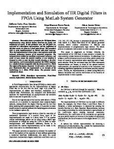
Note that the interfacing of this all-digital module with the rest of the subsystems means handling the controlled decimation of interpolated samples. The all-digital timing recovery block works with two samples per symbol at the input and, as the theory says, it should perform decimation by 2 in order to output data at symbol rate. In this case however, the equalizer that follows at its output requires also two samples (it acts at sample rate); therefore, no slaved decimation by 2 shall be done. A problem arises when the receiver clock is slower than the transmitted one; usually the only sample obtained is passed to the output, but in this case two samples should be “created” and passed to the next stage in a single clock cycle. The all digital timing recovery was successfully tested in simulations with finite arithmetic and a similar result was observed in the first stand-alone tests that have been carried out in the FPGA. Figure 11 illustrates the situation when the receiver clock is faster than the transmitted one; in this case a flag (FLAG RX FAST) indicates this situation and control the rest of the blocks in the structure in order to not consider it for the computations. The lower part of the figure shows the increment of the fractional delay in time. It shows that the flag is activated when the fractional delay recycles from the maximum (1) to the minimum value (0).
VIII. BIOGRAPHIES
Boolean output
Flag RX FAST 1
0
360.01
384.02
408.02
432.02
456.02
480.02
456.02
480.02
Fractional delay (u) 1
0
360.01
384.02
408.02
432.02
Time scale at receiver [µs] Fig. 11. All digital timing recovery, receiver clock is faster than transmitter clock, flag indicates that one sample should not be considered. Nominal receiver clock frequency= 83.33 MHz.
Even though a simulation display is shown here, the same behaviour has been observed in a digital oscilloscope in a real test with the first hardware version of the system. Nevertheless, the interfacing of this block with the rest of the subsystems of the receiver is still under design.
VI. ACKNOWLEDGEMENTS The authors would like to acknowledge the economical support of, and the fruitful discussions with. the PhotonLab Staff at ISMB, Torino, Italy.
VII. REFERENCES
[1]
[2] [3]
[4] [5]
[6]
[7] [8]
Meyr Heinrich, Marc Moeneclaey, and Stefan A. Fechtel, “Digital Communications Receivers: synchronization, channel estimation and signal processing”. Vol. 2. 1998: John Wiley & Sons. U.Mengali, A.N.D'Andrea, Synchronization Techniques for Digital Receivers. 1997, New York: Plenum Press. K. H. Mueller and M. Müller, Timing Recovery in Digital Synchronous Data Receivers. IEEE Trans. Commun., May 1976. COM-24: p. 516531. M. Oerder and H. Meyr, Digital Filter and Square Timing Recovery. IEEE Trans. Commun, May 1988. COM-36: p. 605-612. Gardner, F.M., A BPSK/QPSK timing-error detector for sampled receivers. IEEE Transactions on Communications, 1986. CM-34(5): p. 423. . M. Oerder and H. Meyr, Derivation of Gardner’s Timing Error Detector from the Maximum Likelihood Principle. IEEE Trans. Commun., June 1987. COM-35: p. 684-685. Gardner, F.M., Interpolation in digital modems. I. Fundamentals. IEEE Transactions on Communications, 1993. 41(3): p. 501. Gardner, F.M., Phaselock Techniques. Third ed. 2005, New York: Wiley.
Daniel Cárdenas received the Eng. degree in telecommunications engineering from Escuela Politécnica Nacional, Quito, Ecuador, and the M.Sc. (optical communications) and Ph.D. (electronics engineering) from Politecnico di Torino, Torino, Italy in 2004 and 2008, respectively. He is a coauthor of a patent in the field of telecommunications over plastic optical fibers. He collaborated with Istituto Superiore Mario Boella, Torino, Italy and he was a external consultant for Francecol, France, and Siemens, Germany. He is currently with USFQ, Ecuador. His current research activities include polymer-optical-fiber-based access systems, and digital signal processing techniques and their implementation on FPGA/DSP.
Germán Arévalo received the Eng. degree in telecommunications engineering from Escuela Politécnica Nacional, Quito, Ecuador, and the M.Sc. in optical communications and photonic technologies from Politecnico di Torino, Torino, Italy in 2004. He is now the dean of the electronics faculty, Universidad Politécnica Salesiana, Quito, Ecuador and collaborates with the design center of SAI Technologies Ltd., Ecuador.