Computational Methods for Parameter Estimation in Climate Models

Bayesian Analysis (2008)

3, Number 4, pp. 823–850

Computational Methods for Parameter Estimation in Climate Models Alejandro Villagran∗ , Gabriel Huerta† , Charles S. Jackson‡ and Mrinal K. Sen§ Abstract. Intensive computational methods have been used by Earth scientists in a wide range of problems in data inversion and uncertainty quantification such as earthquake epicenter location and climate projections. To quantify the uncertainties resulting from a range of plausible model configurations it is necessary to estimate a multidimensional probability distribution. The computational cost of estimating these distributions for geoscience applications is impractical using traditional methods such as Metropolis/Gibbs algorithms as simulation costs limit the number of experiments that can be obtained reasonably. Several alternate sampling strategies have been proposed that could improve on the sampling efficiency including Multiple Very Fast Simulated Annealing (MVFSA) and Adaptive Metropolis algorithms. The performance of these proposed sampling strategies are evaluated with a surrogate climate model that is able to approximate the noise and response behavior of a realistic atmospheric general circulation model (AGCM). The surrogate model is fast enough that its evaluation can be embedded in these Monte Carlo algorithms. We show that adaptive methods can be superior to MVFSA to approximate the known posterior distribution with fewer forward evaluations. However the adaptive methods can also be limited by inadequate sample mixing. The Single Component and Delayed Rejection Adaptive Metropolis algorithms were found to resolve these limitations, although challenges remain to approximating multi-modal distributions. The results show that these advanced methods of statistical inference can provide practical solutions to the climate model calibration problem and challenges in quantifying climate projection uncertainties. The computational methods would also be useful to problems outside climate prediction, particularly those where sampling is limited by availability of computational resources. Keywords: Parametric Uncertainties, Inverse Problems, Simulated Annealing, Adaptive Metropolis, Climate Models

1

Introduction

Monte Carlo inversion techniques were first used by Earth scientists more than 30 years ago as a method to estimate the parameters of computer models that simulate real, physical systems. Given randomly selected parameter values the best computer model ∗ Department

of Mathematics and Statistics, The University of New Mexico,Albuquerque, NM of Mathematics and Statistics, The University of New Mexico,Albuquerque, NM, http://www.stat.unm.edu/~ghuerta/ ‡ Institute for Geophysics, University of Texas, Austin, TX, http://www.ig.utexas.edu/people/staff/charles/ § Institute for Geophysics, University of Texas, Austin, TX, http://www.ig.utexas.edu/people/staff/mrinal/ † Department

c 2008 International Society for Bayesian Analysis

DOI:10.1214/08-BA331

824

Parameter Estimation in Climate Models

results were tested for its fit to the observed data and then the model was accepted or rejected to finally make predictions about the physical system of interest. As more computational power became available, Monte Carlo methods have shown to be important in the analysis of nonlinear inverse problems where simple gradient descent algorithms fail and multi-modality of the cost function results in multiple possible solutions. Monte Carlo techniques can be divided as sampling methods and as optimization methods. Monte Carlo sampling is useful where calculus-based methods fail to search an optimal solution and characterize uncertainty. The Metropolis algorithm and the Gibbs sampler are the most widely used Monte Carlo samplers for this purpose. Monte Carlo optimization methods are powerful tools when searching for global optimal solutions amongst numerous local optima. Simulated annealing and genetic algorithms have shown their strengths in this respect. One area of paramount importance for having more quantitative approaches to evaluating parametric uncertainties in Earth sciences is prediction of global warming. Models referenced by the Intergovernmental Panel on Climate Change (IPCC) Third Assessment Report (TAR3) (McCarthy et al. (2001)) predict that global temperatures are likely to increase by 1.1 to 6.4◦ C (2.0 to 11.5◦ F) between 1990 and 2100. The uncertainty in this range comes from both the difficulty in predicting the amount of future greenhouse gas emissions and uncertainties regarding climate sensitivity. There has been limited progress in understanding and quantifying sources of this uncertainty. What has been done stems mainly from the analysis of multiple model responses to similarly applied forcings (e.g. Gates et al. (1999); Joussaume and Taylor (2000); Meehl et al. (2000)). The 2001 IPCC report, in its assessment of current research needs, calls for “a much more comprehensive and systematic system of model analysis and diagnosis, and a Monte Carlo approach to model uncertainties associated with parameterizations” (Section 8.10, McAvaney et al. (2001)). There has been some recent progress along these lines including work with models of reduced complexity (Forest et al. (2000, 2001, 2002)) and perturbed physics ensembles with a general circulation model (Allen (1999); Murphy et al. (2004); Stainforth et al. (2005); Collins et al. (2006); Jackson et al. (2008)). A large disparity exists among various climate models in their prediction of global mean surface air temperature when atmospheric CO2 is doubled compared to present concentrations. There is an overwhelming number of reasons why these differences could exist. Although each climate model has been optimized to reproduce observational means, each model contains slightly different choices of model parameter values as well as different parameterizations of under-resolved physics. Multi-model systems could be more reliable than single-model systems. In this matter, Tebaldi et al. (2005) propose a Bayesian statistical model that combines information from a multi-model ensemble of atmospheric ocean general circulation models (AOGCM) and observations to determine the probability distribution of future climate change. Barnett et al. (2006) use multiple versions of the HadAM3 GCM to quantify the uncertainty in changes in extreme event frequency in response to doubled CO2 . Collins et al. (2006) also compare multi-model ensembles of models from the AR 4 (Parry et al. (2007)) with the predictions using the HadCM3 to quantify uncertainties in transient climate change using a

Villagran, Huerta, Jackson, Sen

825

perturbed physics approach in which modeling uncertainties are sampled systematically by perturbing uncertain parameters. Lopez et al. (2006) develop a Bayesian statistical model to produce probabilistic projections of regional climate change using observations and ensembles of GCMs. Kettleborough et al. (2007) discuss a method for estimating uncertainty in future climate change using Monte Carlo Sampling. A range of model hierarchies have been used to quantify the sources and impacts of climate modeling uncertainties: general circulation models, models of reduced complexity, and surrogate or emulator models. General circulation models are the most demanding computationally and simulate the detailed interactions among the atmospheric, oceanic, land surface, and sea ice components of the climate system and are usually developed by national model development centers such as the Hadley Center and their version 3 coupled Atmosphere-Ocean system (HadCM3) and the National Center for Atmospheric Research and their version 3 Community Climate System Model (CCSM3). As an example of the typical computational expense of these models, it takes 16 processors of a computational cluster 24 hours to simulate 10 years of climate. This expense has motivated some researchers to consider models of reduced complexity where one or more spatial dimensions of a climate model are eliminated (e.g. Forest et al. (2000, 2001, 2002) ). The present work uses a surrogate climate model that mimics the equilibrium space-time response of an Atmospheric GCM to changes in multiple model parameters from a set of previously run experiments to test different sampling strategies for quantifying parametric uncertainties. However, the computational algorithms studied in this paper can be applied in general to find posterior distributions in any statistical inference problem. The methods used are in no way standard for the current state of the art within the climate literature. By applying adaptive methods we can approximate the posterior probability distribution (PPD) of the climate model parameters with few forward evaluations. The results obtained not only could be used to improve the calibration of a climate model but also to test the strength of scientific inferences from observational data. Moreover, the strategically chosen samples could also serve as the basis for creating a statistical climate emulator model on which other, more standard MCMC sampling strategies could be used for generating accurate measures of the posterior distribution. In Section 2, we will review some details on the computer climate model proposed by Jackson and Broccoli (2003). In Section 3, we mention some computational algorithms used to solve inverse problems. In Section 4, we present a comparison between Multiple Very Fast Simulated Annealing (MVFSA) and adaptive methods for the climate model. Finally, Section 5 provides some conclusions.

2

Climate Model

Milankovitch (1941) proposed that variations in the Earth’s orbit cause climate variability through a local thermodynamic response to changes in insolation. The Earth’s orbital geometry parameters (obliquity, longitude of perihelion and eccentricity) are astronomical factors that influence the timing and intensity of the seasons. The properties

826

Parameter Estimation in Climate Models

of the solar forcing result from variations in the obliquity of the Earth’s spin axis relative to the plane of the Earth’s orbit about the Sun, precession of the Earth’s spin axis, and the eccentricity (non-circularity) of the Earth’s orbit. The obliquity varies on a time cycle of about 40,000 yrs. This changes the geographical distribution of insolation on both a seasonal and annual mean basis. When obliquity is high, the summer and annual mean high latitudes receive more insolation, while less is received elsewhere. The Earth’s spin axis completes one precessional cycle in about 20,000 yrs. The precession effect acts to increase insolation during the season the Earth is at its closest approach to the Sun (the perihelion). Because insolation is greater for all latitudes at perihelion, the precessional forcing is in phase globally for any given time of year. Unlike obliquity, precession does little to alter the geographical distribution of annual mean insolation. Variations in eccentricity, occurring on approximately 100,000 year time scales, has a small influence on annual mean insolation. Their main effect is to modulate the strength of the precessional forcing. Jackson and Broccoli (2003) take advantage of the short equilibration time (10 years) of an atmospheric general circulation model (AGCM), land surface model and a static mixed-layer ocean model, which includes a thermodynamic model of sea ice to derive the equilibrium climate response to accelerated variations in Earth’s orbital configuration over the past 165,000 years. By fitting a time series structure of the evolution of each orbital component with the model output, they can estimate an amplitude for each component. This amplitude represents the sensitivity of the region and season to changes in that orbital component. The sensitivity of surface air temperature to obliquity forcing Ao,ijk and precessional forcing Ap,ijk can be defined for particular latitudes i, longitudes j, and seasons k. They correspond to the climate model’s response to the seasonally and latitude varying changes in insolation due to a given unit change in orbital parameter values. They are derived from an ordinary multiple least squares fitting procedure between modeled variations in climate found within a climate model integration of the past 165,000 years forced only by changes in Earth’s orbital geometry and two basis functions representing the known temporal variations in obliquity and precession. In particular, the obliquity basis function Ao,ijk Φ0 (t) consists of an unknown sensitivity Ao,ijk and the time series of obliquity variations Φ0 (t) over the past 165 kyrs. The precessional basis function Ap,ijk e(t)cos(φp,ijk − λ(t)) consists of an unknown sensitivity Ap,ijk , an unknown phase angle of response φp,ijk , the time series of eccentricity e(t), and the time series of the longitude of the perihelion λ(t). The time series e(t), λ(t), and Φ0 (t) are known from orbital mechanics and were used as input values in the AGCM which calculates the changes in insolation as a function of latitude and season for each year of the experiment. The least squares fitting procedure provides estimates of Ao,ijk , Ap,ijk , and φp,ijk that best represent the climate model’s response to the time evolving changes in orbital forcing. Let Tijk (t) represent the variations in surface air temperature with respect to the 165 kyr mean for a given region and season represented by, Tijk (t) = Ao,ijk Φ0 (t) + Ap,ijk e(t)cos(φp,ijk − λ(t)) + Rijk (t)

(1)

Villagran, Huerta, Jackson, Sen

827

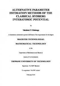
The fitting procedure described above also allows one to construct a surrogate climate model using the estimated latitude, longitude, and seasonal obliquity and precessional forcing sensitivities. Figure 1 gives a comparison of the ability of the surrogate climate model with imposed time variations in Earth’s orbital geometry to reproduce the AGCM’s response of the annual mean air termperature in Antarctica averaged from 70◦ S to 90◦ S and separated into its obliquity, precessional, and residual components. This is done by averaging together the sensitivities of all latitude, longitude, and seasons for this region and estimating the response by imposing the changes in the obliquity and precessional components. We will use this surrogate climate model to test sampling strategies as a followon study to Jackson et al. (2004), which considers the same surrogate model as in this paper but mostly compares Multiple Very Fast Simulated Annealing (MVFSA) with the Metropolis/Gibbs and Grid search algorithms. One of the main goals of our paper is to evaluate factors affecting the efficiency and accuracy of alternate sampling strategies to the MVFSA and Gibbs/Metropolis algorithms. We denote the Earth’s orbital geometry parameters and their physical range as obliquity, Φ ∈ (22◦ , 25◦ ), eccentricity, e ∈ (0, 0.05) and longitude of perihelion, λ ∈ (0◦ , 360◦ ). The observed data is a 3D array dobs,ijk which represents the observed surface temperature anomalies with respect to the long term 165 kyrs mean at latitude i, longitude j, and season k. The grid spacing is approximately 4.5◦ latitude by 7.5◦ longitude, then the latitude can take I = 40 different values, and the longitude J = 48. The season takes K = 12 values, which are selected days throughout the year. Each value of k would apply for that season for all time t over the past 165,000 years. The observed data are simulated using Φ = 22.625, e = 0.043954, and λ = 75.93, as ideal values for the climate model. We approximate the data using the relationship, dobs,ijk = gijk (m) + ηijk , where m = (Φ, e, λ) is the vector of parameters. In this paper, gijk (m) denotes the surface air temperature anomaly as a funcion of the parameters that define the Earth’s orbital geometry. The term ηijk is a Gaussian error with estimated variance given by Bijk , this array represents the variance of the observations at each grid point. This variability comes from the 1,500 year integration of the model itself, but with the appropriate seasonal and climatological averages (i.e. 10 year means of particular seasons). Typically, in Earth science models the observational uncertainties are assumed as Gaussian, see Jackson et al. (2004), Tebaldi et al. (2005) and Lopez et al. (2006). The surrogate climate model is defined as follows, ˆ ijk gijk (m) = Aˆo,ijk Φ0 + eAˆp,ijk cos(φˆp,ijk − λ) + R

(2)

where Φ0 = Φ − Φo is the deviation of obliquity from its 165,000 year mean (Φo = ˆ ijk are the 23.3515◦), φˆp,ijk is the phase of the response to precessional forcing and R residuals averaged over time obtained from (1). This term is added to represent the effects of internal variability on 10 year seasonal means. Repeated experiments of the ˆ ijk that come from a climate model will cycle through 1 of 150 possible values of R ˆ ˆ 1,500 year long control integration of the AGCM. Ao,ijk and Ap,ijk are the sensitivity of temperature to changes in obliquity and precession obtained via the time series fitting

828

Parameter Estimation in Climate Models

procedure in (1). The cost function or misfit function is a measure of the deviation generated from the observed data and the data generated from the model. The cost function can be defined in many ways, for instance for the climate model considered here, I

E(m) =

J

K

1 X X X −1 Bijk (dobs,ijk − gijk (m))2 2 i=1 j=1

(3)

k=1

In general, we can have N different sets of observations. On the climate model studied here there is just one field, surface air temperature anomalies. However, other fields may be used, such as seasonal and annual mean surface air temperature, precipitation, winds, and clouds at different latitudes. Other representations of E(m) are still under investigation. The likelihood function takes the form, L(dobs |m, S) ∝ exp{−SE(m)} where dobs represents the vector of all the data observations.. The parameter S is connected to Bijk according to Jackson et al. (2004) as a scaling factor. S performs the function of weighing the significance of model-data differences. Large values of S would imply small errors between the data and the model and would result in highly peaked probability distributions. To illustrate this, we fixed S = 47 based on the expertise and initial knowledge given in Jackson et al. (2004) as an appropriate value for this parameter. To gain some initial insight of the likelihood function for the surrogate climate model, we can plot the profile likelihood for each parameter. Since we already know the optimal values for the simulation study about this model (Φ = 22.625, e = 0.043954, λ = 75.93), we fix two parameters at their optimum value and we evaluate the third one using a 20,000 point grid evaluation. Figure 2 shows the profile likelihoods for each parameter, Φ, e and λ for two different values of S. Due to internal variability, the climate model can take a range of likelihood values for any given combination of orbital parameter values. This scatter from internal variability (noise term in equation 2) is seen within Figure 2 as the thin vertical lines that follow the broader scale variations in likelihood values. These broad scale variations reflect the smoothly evolving changes in climate that accompany changes in orbital geometry.

3

Computational Approaches

3.1

Metropolis/Gibbs

Geman and Geman (1984) consider that a Gibbs distribution π can be uniquely determined by π(ω) π(xs |xr , r 6= s) = P s ∈ S, ω ∈ Ω. xs ∈∆ π(ω)

Where S = {s1 , ..., sN } is a set of sites and Ω = {ω = (xs1 , ..., xsN )| xsi ∈ ∆, 1 ≤ i ≤ N } is the set of all possible configurations. In geosciences, Sambridge and Mosegaard (2002), uses the right side of this formula to define the Gibbs sampler algorithm while

Villagran, Huerta, Jackson, Sen

829

Gelfand and Smith (1990) proposed to use the left side to iteratively sample the full conditionals of each parameter. The Gibbs sampler is a version of an importance sampling technique that improves the efficiency of the calculation by sampling model parameter sets from the Gibbs distribution which is, in effect, equivalent to the desired posterior probability distribution (PPD). This approach requires the parameter space to be subdivided into a number of equally spaced intervals. The Metropolis-Hastings (M-H) algorithm (Hastings (1970)) is a variation of the Metropolis scheme (Metropolis et al. (1953)), which requires a probability function q as a proposal. This proposal or jump distribution affects the way in which new models are accepted. The rule is to accept a new model m(k+1) with probability,   π(m(k+1) )q(m(k+1) , m(k) ) . α(m(k) , m(k+1) ) = min 1, π(m(k) )q(m(k) , m(k+1) ) Another version of the Metropolis algorithm proposed by Sen and Stoffa (1996) is the Multiple Metropolis Simulated Annealing (METSA). This method is started from several independent initial points to improve the sampling of π. At every point, candidates are drawn at random. The acceptance/rejection rule is affected by using a cooling schedule T on P = exp(−∆E/T ), where ∆E = E(m(k+1) ) − E(m(k) ). Adding T allows to sample regions of the parameter space with high density.

3.2

Multiple Very Fast Simulated Annealing (MVFSA)

One may use the temperature parameter within the Metropolis algorithm to take advantage of the well known features of stochastic optimizers from Simulated Annealing (Kirkpatrick et al. (1983)) and the Very Fast Simulated Annealing (Ingber (1989)) to locate the global minimum in the cost function E(m) by very slowly lowering the temperature parameter. Ingber (1989) propose the selection of model parameters given a (k) (k+1) (k) ), yi is − mmin current selection mi within VFSA so that mi = mi + yi (mmax i i generated according to a Cauchy distribution which is dependent on the cooling schedare the ule at iteration k, Tk = To exp(−α(k − 1)1/d ). The scalars mmax and mmin i i maximum and minimum values that the parameter i can take. The acceptance criterion for successive model selections is the same as for the Metropolis algorithm. Also Sen and Stoffa (1996) and Jackson et al. (2004) argue that one may allow for numerous repetitions of the minimization procedure to strike a balance between estimating a multidimensional PPD and finding the global minimum. This is known as the MVFSA algorithm which has the following features: • Optimization: Take advantage of the well known characteristics of stochastic optimizers from Simulated Annealing (SA) and VFSA. • Multiple: Instead of using a single initial value as SA or VFSA, we can use “multiple” initial values over the parameter space. • Sampling: For each single initial value, propose a new candidate using a random walk combined with a random number sampled from a Cauchy distribution that

830

Parameter Estimation in Climate Models is dependent on the cooling schedule. Acceptance of the proposed value is similar to a Metropolis step.

• Flexibility: Two additional parameters such as moves/temperature and ntarget add flexibility to the VFSA algorithm to control sampling efficiency for a specified number of dimensions. Although MVFSA sampling is based on stochastic optimization, the PPD derived through the MVFSA algorithm is broader than what may be obtained through the Metropolis/Gibbs sampler as a result of the multiple independent initial values over the parameter space.

3.3

Adaptive Methods

The computational effort of evaluating the cost function in climate models has made the Metropolis/Gibbs traditional schemes useless in this context. On the other hand, the MVFSA algorithm provides fast, approximate but biased answers to solve the problem of mapping the multidimensional PPD. In order to reach a balance between efficiency and precision we consider the use of adaptive methods. One of the issues with the Metropolis or the Metropolis-Hastings algorithm is the choice or tuning of an effective proposal distribution to keep acceptance rates at a 40 − 60% level. Alternatively Haario et al. (1999) suggested a method called Adaptive Proposal (AP) that basically updates the proposal distribution with the knowledge we have so far learned about the target distribution. Furthermore Haario et al. (2001) proposed a variation of the AP algorithm called Adaptive Metropolis (AM) which is a non-Markovian algorithm but has ergodic properties. The AM has two versions, one called Single Component Adaptive Metropolis (SCAM) and the full component version (FAM). Haario et al. (2004) applied the SCAM algorithm to a 90 dimension inversion problem about gas profiles (GOMOS) in a successful way. Another powerful variant is called Delayed Rejection Adaptive Metropolis (DRAM) that combines the Delayed Rejection scheme (Tierney and Mira (1999)) with the AM. SCAM Let π denote the density of our target distribution, typically a PPD which we can evaluate up to a normalizing constant. The sequence m(0) , m(1) , ... denotes the full states of the process, that is, we consider a new state updated as soon as all the d components (0) (k−1) of the state have been separately updated. We denote mi,k−1 = (mi , ..., mi ) as the sampled vector for the i-th parameter up to state k − 1. The adaptive scheme is (k) done through the variance equation Vi = sd V (mi,k−1 ) + sd , where V (mi,k−1 ) = P P (r) (r) k−1 k−1 1 1 2 − mi ) , mi = k r=0 mi , sd is a positive constant and 0 <  < 1. r=0 (mi k−1 (k)

When updating on the i-th parameter mi

at state k, we apply a one dimensional

Villagran, Huerta, Jackson, Sen

831

Metropolis step: • Sample

(k−1)

zi ∼ N (mi

(k)

, Vi

)

• Accept the candidate point zi with probability (k)

min 1,

(k)

in which case we set mi

(k)

(k−1)

(k−1)

π(m1 , ..., mi−1 , zi , mi+1 , ..., md (k)

(k)

(k−1)

π(m1 , ..., mi−1 , mi

(k)

= zi , and otherwise mi

(k−1)

, ..., md

)

(k−1)

= mi

)

!

.

In the case of the climate model described previously, we generated samples from the posterior distribution of interest π(m, S|dobs ) using a two step scheme. We considered flat priors on all the orbital forcing parameters and since S can be thought of as a precision parameter, we choose a Gamma(α0 , β0 ) distribution as a prior for S. The hyperparameters α0 = 552.25 and β0 = 11.75 were fixed by expertise to provide a prior mean E(S) = 47 and a prior variance V ar(S) = 4. This issue will be discussed in Section 4.3. Therefore π(m|S, dobs ) is sampled according to the SCAM algorithm and as a second step, we sample from π(S|m, dobs ) which is a Gamma distribution with parameters α∗ = α0 and β ∗ = β0 + E(m(k) ). When the parameters of the target function are highly correlated the SCAM can suffer from poor mixing. A remedy to this problem is to rotate the proposal distribution during the early stage of the sampling (i.e. during the burn-in period). The rotation can be done by computing the covariance matrix of the chain so far detected and then computing the eigenvalues of this matrix. We sort the eigenvalues from the largest to the smallest and we use this ordering to define sampling directions for the parameters in the SCAM algorithm. FAM Suppose that at time t − 1 we have sampled the states m(0) , ..., m(t−1) where m(0) is the initial state and is a vector of dimension d. Then a candidate point z is sampled from the proposal distribution qt (·|m(0) , ..., m(t−1) ), which now may depend on the whole history. The candidate z is accepted with probability,   π(z) , α(m(t−1) , z) = min 1, π(m(t−1) ) in which case we set m(t) = z, and otherwise m(t) = m(t−1) . The proposal distribution qt (·|m(0) , ..., m(t−1) ) employed in the FAM algorithm is a multivariate Gaussian distribution with mean at the current point m(t−1) and covariance matrix Ct . The matrix Ct is computed using the sampled covariance matrix of the parameters up to iteration t. The crucial aspect regarding the adaptation is how the covariance of the proposal distribution depends on the history of the chain. In the

832

Parameter Estimation in Climate Models

FAM algorithm this is handled by setting Ct = sd Ct−1 + sd Id after an initial period, where sd is a positive constant that depends only on the dimension d and  > 0 is a constant that we may choose very small but positive. The role of  is to ensure that C t does not become singular. As a basic choice for the scaling factor sd we can adopt the value sd = (2.4)2 /d as in Gelman et al. (1996). In difference to the SCAM algorithm all parameters are sampled at once in the FAM scheme. The AM chain defined above simulates properly the target distribution π regardless of the initial distribution. For a detailed proof of this result, see Haario et al. (2001). DRAM Haario et al. (2006) combine the ideas of Delayed Rejection (DR) and Adaptive Metropolis to improve the efficiency of MCMC algorithms. The general idea of DR is that upon rejection for the M-H algorithm, instead of advancing time and retaining the current position, a second stage move is proposed. The acceptance probability of the second stage candidate is computed so that reversibility of the Markov chain relative to the distribution of interest is preserved. The process of delaying rejection can be iterated for a fixed or random number of stages. The DR can be also considered as a way of mixing different proposals to allow the sampler to explore the parameter space more efficiently. There is a number of different strategies to combine DR and AM. One idea is to use DR only for the burn-in period and discard the part of the chain where DR has been used. These iterations can be thought as an automatic burn-in period. In this paper, we implemented DRAM in the following way. We updated the first stage proposal covariance matrix Ct for a very short number of iterations via AM exclusively. After this point, if a proposed value z ∗ under AM is rejected, we then compute a second stage proposal Vt = hCt where h is a specified constant. Then, we propose a new point from a multivariate normal distribution with mean vector z ∗ and covariance matrix Vt . The best results with the climate model were achieved when h ≤ 0.01.

4

MVFSA and Adaptive Methods in Climate Model

We now compare the five different computational techniques presented in Section 3 in the context of the climate model described in Section 2. One of our goals is to provide alternatives to traditional algorithms such as the Gibbs sampler and the MetropolisHastings that have little chance to succeed in a climate model inverse problem either because they need several forward evaluations, or because of the difficulty to find a good proposal distribution. One of the main concerns on climate models is the time spent in performing forward evaluations. We did several runs of 100,000 iterations to estimate the time in seconds that every method uses to make one forward evaluation for the climate model. We found there is no significant difference among FAM, METSA and MVFSA which only require a single model evaluation for each iteration. DRAM is slower than these three algorithms

Villagran, Huerta, Jackson, Sen

833

because of the delayed rejection and possible use of multiple model evaluations per iteration. SCAM is three times slower than FAM as the number of model evaluations equals the dimension of the parameter space d = 3. We looked at the bivariate scatter plots of the samples from the different methods corresponding to each orbital parameter. For the adaptive methods, we use a burn in period of 20,000 iterations while in the case of MVFSA and METSA there is no burn in period and their sampling design is based on multiple independent starting points over the parameter space. These scatter plots reveal that all methods sample the regions of the parameter space where the optimum is located. However, the dispersion of the samples based on the Simulated Annealing methods is higher than the one from adaptive methods. While the adaptive methods use one single point and adapt themselves to reach the target distribution, the MVFSA and METSA need to start at different independent initial points to collect all the information that they require to estimate the PPD.

4.1

Root Mean Square (RMS) Probability Error

Besides assessing the time that each method uses to make forward evaluations of the climate model we consider an empirical measure of convergence for any proposed algorithm. For every parameter θ, the RMS probability error is defined as follows: (θ)

RM Si (θ) = ||P robi

− P rob(θ) π ||

where i goes from 0 to the maximum number of iterations and ||·|| denotes the Euclidean (θ) norm. P robi is a vector that contains the frequencies to plot a histogram using the samples generated from a specific method (FAM, SCAM, DRAM, MVFSA or METSA) (θ) at iteration i. P robπ is a vector of frequencies from the target distribution π based on (θ) the same bins used for P robi . Since we do not have available the actual frequencies based on π, we replace them by those obtained with the whole sample simulated from the FAM since this algorithm has ergodic properties. RMS has the desired property that it goes to zero as i goes to infinity when the method being used converges to the target distribution. The RMS also provides a measure of how fast an estimated PPD from the samples of any particular method stops changing over iterations. In Figure 3, we show that every method provides a PPD centered on the target value of obliquity, Φ = 22.625. MVFSA and METSA provide a distribution with long tails due to their design based on multiple initial values and Simulated Annealing compared to the distribution of obliquity obtained with FAM, SCAM and DRAM. A goal for climate models is to estimate properly the uncertainty about parameters of interest. For instance, we consider the estimation of the 97.5% quantile for every parameter. In Figure 3, we also show the estimated 97.5% quantile per iteration and for all the methods. The quantile estimation via MVFSA and METSA is at a value of 24.2, while with the other methods the estimated quantile is at 23. One comment in Sen and Stoffa (1996) and Jackson et al. (2004) is that MVFSA is

834

Parameter Estimation in Climate Models

preferred over Metropolis/Gibbs algorithms because of the reduction in the number of forward evaluations and the time needed to estimate the PPD. In the middle graphs of Figure 3, we can see that DRAM and SCAM have the lowest RMS up to iteration 30,000, after which FAM has the minimum RMS value. The RMS values of MVFSA converge as quick or quicker than those of DRAM and SCAM but they do not reach zero. One concern with the RMS as a measure to compare how fast the algorithms converge to the target distribution, is that it is presented as a function of the iterations. This could be misleading since it does not consider that every method requires a different number of model evaluations to make one iteration. To overcome this issue we propose to look at the RMS as a function of time. In this case DRAM fairs better than SCAM within the first hundreds of seconds. Perhaps the most surprising aspect of these results is the slow convergence rate of FAM. One would have expected FAM to be fast, similar to the DRAM and SCAM results, since it integrates information about previous samples to generate an improved proposal distribution. We hypothesize that the calibration of the covariance matrix for the proposal distribution in this problem is particularly difficult because of the need to restrict orbital forcing parameter values to a particular range. We suspect that the DRAM algorithm is able to overcome this problem by adding a second stage proposal with more precision which allows us to improve the mixing at the beginning of the algorithm. It is not entirely clear to us why SCAM was able to perform so well relative to FAM. However, SCAM handles one parameter at each stage and therefore it is simpler to deal both with the parameter physical restrictions and with the correlation among parameters. For the Longitude of Perihelion parameter, Figure 4 shows similar results as described for the previous Figure. In this case DRAM and SCAM converge as fast to an answer compared to MVFSA and METSA. The estimated 97.5% quantile via MVFSA and METSA is now 3 times greater than the same estimated quantile for the other methods. In Figure 5, for the Eccentricity parameter, FAM and SCAM have some differences on the estimation of the PPD, this is because the FAM uses as a proposal distribution a multivariate normal density which could lead into many rejections of new candidates points due to the physical restrictions on the orbital forcing parameters. On the other hand, the estimated PPD under DRAM is similar to the one obtained via SCAM. For the Eccentricity parameter, there are no differences on the estimation of the 97.5% quantile. However, this is not the case for the estimation of the 2.5% quantile as we can see from the box plots at the bottom of the Figure. We looked at the sample autocorrelation function (ACF) of each parameter for all the algorithms that are being considered. This is a well known way to assess how every algorithm is mixing along iterations, the smaller the autocorrelations the better the method is moving across the parameter space. We noticed that FAM has the worst autocorrelations, this is no surprise since the algorithm is sampling all the parameters at once from a multivariate Gaussian distribution and the physical restrictions on each parameter make difficult to achieve acceptances that satisfy the restrictions. By using DRAM, we reduce the autocorrelations of the FAM but they are not as good as the autocorrelations of SCAM. In fact, SCAM is very efficient in terms of chain mixing even though it is the slowest one in computer time spent per forward evaluation. The

Villagran, Huerta, Jackson, Sen

835

adaptive methods have acceptance rates at around 45%. METSA and MVFSA are similar in terms of autocorrelation, their autocorrelation function values are not so large because the sampling design on these algorithms is based on multiple initial points that are not connected to each other along the iterations.

4.2

Appraisal of a few forward evaluations on the surrogate climate model

Even though the surrogate climate model used in this paper is cheap enough to make forward evaluations without consideration of the execution time, climatologists have an interest in making inferences about models that may take hours to days to execute a single iteration of a stochastic sampler. In these cases one may only have a limited number of samples to work with. Looking for an algorithm that is efficient to sample from becomes a mandatory task. From a statistical standpoint, a statistical climate model or emulator can avoid computational limitations as shown in Sans´ o et al. (2008). Depending on the problem characteristics, this may not always be an easy task especially if the region of acceptability is a small fraction of the parameter space volume. Therefore, inefficient samplers fail to capture the most important regions. We considered a Gaussian spatial model to approximate the surface of the surrogate climate model parameters but we did not obtain good results. We believe this was a result of not having enough information or understanding about the climate model characteristics to formulate a statistical version. Also, stationary models are limited for the output arising from our surrogate model. Therefore, there will likely continue to be a need for efficiently sampling schemes to achieve good inferences with few evaluations. We chose only 500 forward evaluations for testing all the sampling strategies presented in this paper. In Figure 6, we see that based on 500 iterations MVFSA and METSA sample various points over the parameter space, but a few hundreds iterations are not enough to establish a pattern on the bivariate plots. On the other hand, SCAM and DRAM show a very good concentration of the samples. These bivariate plots look much alike the scatter plots we get using the entire run from the adaptive methods. The behavior of the FAM algorithm although disappointing, is expected since the proposal cannot be easily tuned with a small number of iterations. There is no burn-in period considered in the samples of FAM, DRAM and SCAM used to produce this Figure. In Table 1, we compare the uncertainty estimation of the parameters and the minimum values of the cost function. The performance of SCAM and DRAM are remarkable since they not only find a minimum cost with few forward evaluations, but they also provide acceptable estimates of the 95% credible intervals of the orbital forcing parameters. The 95% credible intervals for the methods based on Simulated Annealing are not informative at all because they practically covered the entire parameter space. In Figure 7, we compare the estimation of the marginals using 500 iterations to the estimation made with 100, 000 samples from the FAM. With only 500 iterations, FAM does a poor job estimating the marginals while DRAM and SCAM seem to do a very

836

Parameter Estimation in Climate Models

Method FAM SCAM DRAM MVFSA METSA

E(m∗ ) 0.8411 0.1912 0.1943 0.2019 0.2029

Φ2.5% 22.6817 22.1644 22.1665 22.1595 22.0631

Φ97.5% 22.7813 23.1309 22.9816 24.5072 24.2744

λ2.5% 0.2248 60.6625 62.7528 18.3329 38.6806

λ97.5% 3.4413 91.5434 141.1550 311.9383 353.6220

e2.5% 0.0101 0.0312 0.0113 0.0089 0.0029

e97.5% 0.0331 0.0495 0.0491 0.0482 0.0481

Table 1: Comparative estimation after 500 forward evaluations. E(m∗ ) is the minimum of the cost function, Φ is the Obliquity, λ is the Longitude of Perihelion and e is the Eccentricity. good job for Longitude of Perihelion and Eccentricity. For Obliquity the estimation is acceptable. The factor h on the second stage proposal for DRAM is producing a large impact compared to AM for the results based with only a few iterations. MVFSA and METSA present a lot of mass on the tails in comparison to the results of the FAM with 100,000 iterations. From a practical standpoint, the main problem with FAM is its difficulty to tune up the covariance matrix from the proposal distribution in a parameter space where there are physical restrictions. There are different strategies to combine both the delayed rejection and the adaptive Metropolis algorithms. The strategy that achieves best results for the climate model is to implement the AM for a short number of iterations to compute the covariance matrix Ct of the first state proposal distribution and then construct the matrix Vt = hCt which it has more precision given that we selected h ≤ 0.01. Vt is used in the second stage proposal. By doing this, we allow DRAM the chance to take two different steps: (first stage) one that allows global moves to sample along the parameter space and (second stage) another step that allows to sample with more precision from points in the parameter space where the posterior distributions have more density. Using a small number of forward evaluations we have gained appreciation of how well the computational methods presented in this paper work in this context. The main strengths and weaknesses of every sampling scheme has been emphasized. While Simulated Annealing based sampling schemes present a very good tool to optimize the problem, SCAM and DRAM reach the balance between sampling and optimization with few iterations.

4.3

Relevance of the parameter S

As mentioned in Section 2, the parameter S performs the function of weighing the significance of model-data differences and was included in our inferences of parametric uncertainty. S has its own prior probability distribution that provides information about observational and other uncertainties that are hard to quantify within the metric of model skill E(m) such as correlations among a suite of observations. In Figure 8, we can see what happens if we use a non-informative prior on S, our results only reflect the

Villagran, Huerta, Jackson, Sen

837

form of the likelihood function of each parameter when we set S = 1. In our case, the prior mean value of S is elicited to be 47, a number much larger than 1 which reflects the fact that many surface temperature points are highly correlated. This correlation increases the ability to detect the effects of Earth’s orbital geometry on observations of surface air temperature and sharpens the PPD around the correct orbital configuration. Our results are consistent with the findings of Sans´ o et al. (2008) where they use an emulator of their climate model based on a Gaussian process. They use the MIT 2D climate model that controls the large-scale response of the climate system to external forcings. In that paper, the authors find that when they use non-informative priors on the climate model parameters they obtain vague posteriors. Since S is used to assist on the optimization process of the cost function of the climate model, we may think that it has a positive support. A convenient form for a prior on S is the Gamma probability distribution. The simplicity of this assumption makes possible to sample directly from the full conditional P (S|m, d). More on the interpretation and the motivation of this S parameter can be found in Jackson et al. (2008).

5

Conclusions

Sen and Stoffa (1996) stated that traditional methods such as Metropolis or Gibbs sampler were not sufficiently practical for finding inversion solutions due to their high cost in terms of the time required making forward evaluations and the amount of tuning these algorithms need. MVFSA and METSA were proposed as algorithms to overcome these problems. Indeed they provide approximate and fast answers to estimating the PPD. These methods share the same design based on multiple independent initial starting values, cooling schedule and a Metropolis acceptance rule for new candidates. Adding multiple initial points to these algorithms helps to provide more information about the parameter space similar to a grid point search. They differ in the proposal distribution since MVFSA uses a Cauchy distribution dependent on the cooling schedule to sample candidates from high density regions while METSA uses a random walk proposal and the temperature cooling schedule is present only in the acceptance/rejection step. However, by its design MVFSA has biases estimating the tails of the PPD of the climate model parameters. Annan and Hargreaves (2007) noted that we can consider of either MVFSA or METSA as sophisticated heuristic methods to estimate the PPD. The series of adaptive methods proposed by Haario et al. (1999, 2001, 2004, 2005) are setting a breakthrough in Monte Carlo methods by introducing adaptive schemes that are successful in finding the target distribution not only in theory but also in practice despite the fact that these are non Markovian algorithms. Compared to FAM, DRAM, or SCAM, which all provided nearly identical estimates of the marginal PPD, marginals derived from MVFSA and METSA sampling had similar modes, but with broader 95% credible intervals. For instance, for the Longitude of Perihelion (λ = 75.93) parameter, the 95% posterior credible interval using the FAM scheme is (60.291, 90.676) compared with (23.274, 280.675) that was obtained using MVFSA. The inclusion of the parameter S in the estimation process provides prior

838

Parameter Estimation in Climate Models

information about the significance of model differences with the target observations. As we stated at the beginning of the paper, the main goals of this work were to compare sampling efficiencies and accuracies among different proposed methods for estimating parametric uncertainties. The DRAM and SCAM sampling algorithms are particularly effective on both of these accounts. In terms of the RMS criterion, the adaptive methods were as efficient as MVFSA to reach convergence, but without its sampling biases. The decision to choose either the full component version (FAM) or the single component version (SCAM) of the adaptive methods should be based on the problem at hand. FAM has great speed but also needs to calibrate the covariance matrix of the parameters of interest. As we observed this could be a drawback in parameter spaces with physical restrictions. We propose to employ DRAM when such problem exists and obtained substantial improvements on the results. On the other hand, SCAM does not have to deal with inversion of covariance matrices but it pays a price regarding computational time as soon as the dimensionality of the problem increases. As a caveat, the results obtained from the methods used in this paper only apply to non-linear inverse problems with unimodal posteriors. Finding a good proposal distribution to sample from is difficult even for adaptive methods when the posterior distribution of interest has multiple modes. Ongoing work is being done to develop computational methods that have a balance between sampling a multi-modal PPD and reducing the cost in making forward evaluations in climate models. In terms of efficiency of estimation and ensemble generation in climate modeling, a statistical emulator is a computationally efficient approximation to a complex computer model as mentioned in Annan and Hargreaves (2007) and depicted in Sans´ o et al. (2008). Although, we share the same goals as Sans´ o et al. (2008) our problem is different since we are making evaluations directly on the climate model and not based on a statistical emulator. One can use the results obtained in in this paper to suggest how with relatively few model integrations one may draw inferences of how observational data may constrain uncertain model parameters or physical hypotheses about how nature works. The potential applications are broad and may prove invaluable for problems that are currently limited by computational requirements of the forward model or inordinately large data volumes.

References Allen, M. (1999). “Do-it-yourself climate prediction.” Nature, 401: 642. 824 Annan, J. and Hargreaves, J. (2007). “Efficient estimation and ensemble generation in climate modelling.” Philosophical Transactions of the Royal Society A, 365: 2077– 2088. 837, 838 Barnett, D., Brown, S., Murphy, J., Sexton, D., and Webb, M. (2006). “Quantifying

Villagran, Huerta, Jackson, Sen

839

uncertainty in changes in extreme event frequency in response to doubled CO2 using a large ensemble of GCM simulations.” Climate Dynamics, 26: 489–511. 824 Collins, M., Booth, B., Harris, G., Murphy, J., Sexton, D., and Webb, M. (2006). “Towards quantifying uncertainty in transient climate change.” Climate Dynamics, 127–147. 824 Forest, C., Allen, M. R., Sokolov, A. P., and Stone, P. H. (2001). “Constraining climate model properties using optimal fingerprint detection methods.” Climate Dynamics, 18: 277–295. 824, 825 Forest, C., Allen, M. R., Stone, P. H., and Sokolov, A. P. (2000). “Constraining uncertainties in climate models using climate change detection techniques.” Geophys. Res. Lett., 27(4): 569–572. 824, 825 Forest, C., Stone, P. H., Sokolov, A. P., Allen, M. R., and Webster, M. D. (2002). “Quantifying uncertainties in climate system properties with the use of recent climate observations.” Science, 295: 113–117. 824, 825 Gates, W. L., Boyle, J. S., Covey, C., Dease, C. G., Doutriaux, C. M., Drach, R. S., Fiorino, M., Gleckler, P. J., Hnilo, J. J., Marlais, S. M., Phillips, T. J., Potter, G. L., Santer, B. D., Sperber, K. R., Taylor, K. E., and Williams, D. N. (1999). “An Overview of the Results of the Atmospheric Model Intercomparison Project (AMIP I).” Bulletin of the American Meteorological Society, 80(1): 29–56. 824 Gelfand, A. and Smith, A. (1990). “Sampling-Based Approaches to Calculating Marginal Densities.” Journal of the American Statistical Association, 85: 398–409. 829 Gelman, A., Roberts, G., and Gilks, W. (1996). “Efficient Metropolis jumping rules.” In Bernardo, J., Berger, J., Dawid, A., and Smith, A. (eds.), Bayesian Statistics, volume 5, 599–608. Oxford University Press. 832 Geman, S. and Geman, D. (1984). “Stochastic Relaxation, Gibbs Distributions, and the Bayesian Restoration of Images.” IEEE Transactions PAMI-6, 721–741. 828 Haario, H., Laine, M., Lehtinen, M., Saksman, E., and Tamminen, J. (2004). “Markov Chain Monte Carlo methods for high dimensional inversion in remote sensing.” Journal of Royal Statistical Society, 66: 591–607. 830, 837 Haario, H., Laine, M., Mira, A., and Saksman, E. (2006). “DRAM: Efficient adaptive MCMC.” Statistics and Computing, 16: 339–354. 832 Haario, H., Saksman, E., and Tamminen, J. (1999). “Adaptive proposal distribution for random walk Metropolis algorithm.” Computational Statistics, 14: 375–395. 830, 837 — (2001). “An Adaptive Metropolis algorithm.” Bernoulli, 7: 223–242. 830, 832, 837

840

Parameter Estimation in Climate Models

— (2005). “Componentwise adaptation for high dimensional MCMC.” Computational Statistics, 20(2): 265–263. 837 Hastings, W. (1970). “Monte Carlo sampling methods using Markov chains and their applications.” Biometrika, 57: 97–109. 829 Ingber, L. (1989). “Very fast simulated re-annealing.” Mathematical Computational Modelling, 12: 967–973. 829 Jackson, C. S. and Broccoli, A. (2003). “Orbital forcing of Arctic climate: mechanisms of climate response and implications for continental glaciation.” Climate Dynamics, 21: 539–557. 825, 826 Jackson, C. S., Sen, M., Huerta, G., Deng, Y., and Bowman, K. (2008). “Error Reduction and Convergence in Climate Prediction.” Journal of Climate (in press). 824, 837 Jackson, C. S., Sen, M., and Stoffa, P. (2004). “An Efficient Stochastic Bayesian Approach to Optimal Parameter and Uncertainty Estimation for Climate Model Predictions.” Journal of Climate, 17: 2828–2840. 827, 828, 829, 833 Joussaume, S. and Taylor, K. (2000). “The Paleoclimate Modeling Intercomparison Project (PMIP).” In Braconnot, P. (ed.), Proceedings of the third PMIP workshop, Canada, 4-8 October 1999, WCRP-111, WMO/TD-1007, 271. 824 Kettleborough, J., Booth, B., Stott, P., and Allen, M. (2007). “Estimates of Uncertainty in Predictions of Global Mean Surface Temperature.” Journal of Climate, 20: 843– 855. 825 Kirkpatrick, S., Gelatt, J., and Vecchi, M. (1983). “Optimization by simulated annealing.” Science, 220: 671–680. 829 Lopez, A., Tebaldi, C., New, M., Stainforth, D., Allen, M., and Kettleborough, J. (2006). “Two Approaches to Quantifying Uncertainty in Global Temperature Changes.” Journal of Climate, 19: 4785–4796. 825, 827 McAvaney, B. J., Covey, C., Joussaume, S., Kattsov, V., Kitoh, A., Ogana, W., Pitman, A., Weaver, A., Wood, R., and Zhao, Z. (2001). “Model Evaluation. Climate Change 2001: The Scientific Basis Contribution of Working Group I to the Third Assessment Report of the Intergovernmental Panel on Climate Change.” In Houghton, J., Ding, Y., Griggs, D., Noguer, M., van der Linden, P., Dai, X., Maskell, K., and Johnson, C. (eds.), Third Assessment Report of the Intergovernmental Panel on Climate Change (IPCC), 881. Cambridge University Press,UK. 824 McCarthy, J. J., Canziani, O. F., Leary, N. A., Dokken, D., and White, K. S. (eds.) (2001). Contribution of Working Group II to the Third Assessment Report of the Intergovernmental Panel on Climate Change (IPCC). Cambridge University Press, UK. 824

Villagran, Huerta, Jackson, Sen

841

Meehl, G., Boer, G., Covey, C., Latif, M., and Stouffer, R. (2000). “The Coupled Model Intercomparison Project (CMIP).” Bulletin of the American Meteorological Society, 81(2): 313–318. 824 Metropolis, N., Rosenbluth, A., Rosenbluth, M., Teller, A., and Teller, E. (1953). “Equations of State Calculations by Fast Computing Machines.” Journal of Chemical Physics, 21: 1087–1091. 829 Milankovitch, M. (1941). “Canon of insolation and the ice age problem (Israel Program for Scientific Translations, Jerusalem).” 825 Murphy, J., Sexton, D. M. H., Barnett, D. N., Jones, G. S., Webb, M. J., Collins, M., and Stainforth, D. A. (2004). “Quantification of modelling uncertainties in a large ensemble of climate change simulations.” Nature, 430: 768–772. 824 Parry, M., Canziani, O., Palutikof, J., van der Linden, P., and Hanson, C. (eds.) (2007). IPCC, 2007: Climate Change 2007: Impacts, Adaptation and Vulnerability. Contribution of Working Group II to the Fourth Assessment Report of Intergovermental panel on Climate Change. Cambridge University Press, UK. 824 Sambridge, M. and Mosegaard, K. (2002). “Monte Carlo Methods in Geophysical Inverse Problems.” Review of Geophysics, 40: 1–29. 828 Sans´ o, B., Forest, C., and Zantedeschi, D. (2008). “Inferring Climate System Properties Using a Computer Model (with discussion).” Bayesian Analysis, 3(1): 1–62. 835, 837, 838 Sen, M. and Stoffa, P. (1996). “Bayesian Inference, Gibbs sampler and uncertainty estimation in geophysical inversion.” Geophysical Prospecting, 44: 313–350. 829, 833, 837 Stainforth, D., Aina, T., Christensen, C., Collins, M., Faull, N., Frame, D. J., Kettleborough, J. A., Knight, S., Martin, A., Murphy, J. M., Piani, C., Sexton, D., Smith, L. A., Spicer, R. A., Thorpe, A. J., and Allen, M. R. (2005). “Uncertainty in predictions of the climate response to rising levels of greenhouse gases.” Nature, 433: 403–406. 824 Tebaldi, C., Smith, R., Nychka, D., and Mearns, L. (2005). “Quantifying Uncertainty in Projections of Regional Climate Change: A Bayesian Approach to the Analysis of Multimodel Ensembles.” Journal of Climate, 18: 1524–1540. 824, 827 Tierney, L. and Mira, A. (1999). “Some Adaptive Monte Carlo Methods for Bayesian Inference.” Statistics in Medicine, 18: 2507–2515. 830

Acknowledgments We express our thanks to the Editor, to the Associate Editor and the referee for their comments that had lead into an improved version of this paper. This work has been funded by the National Science Foundation grant OCE-0415251. The first author was also partially supported by the CONACyT-Mexico grant 159764.

842

Parameter Estimation in Climate Models

Villagran, Huerta, Jackson, Sen

843

(a)

(b)

Lowest Level Temperature [K]

Obliquity Component

(c) Precessional Component

(d) Residual

Thousands of years before present

Figure 1: AGCM response of annual and zonal mean lowest level temperature (Kelvin degrees) from 70◦ S to 90◦ S (over Antarctica) to known continuous changes in Earth’s orbital geometry for the past 165 thousand years (e(t), λ(t), and Φ0 (t) are known time series). Panel (a) shows the model response (in gray) with least squares fitted solution (black curve) given by equation (1). The least squares fitted solution includes an obliquity component (b), and precessional component (c). The residual between the least squares fitted solution and the AGCM is shown in panel (d).

844

Parameter Estimation in Climate Models

S=47

S=1

22

23

24

25

22

23

24

25

Obliquity

0

100

200

300

0

100

200

300

Longitude of Perihelion

0

0.01 0.02 0.03 0.04 0.05

0

0.01 0.02 0.03 0.04 0.05

Eccentricity Figure 2: Likelihood for orbital forcing parameters. Left column: S=1. Right column: S=47.

Villagran, Huerta, Jackson, Sen

845

1.8

Quantile Estimation − 97.5%

25

FAM SCAM

1.6

DRAM MVFSA

24.5

METSA

1.4

1.2

Obliquity

24

1

0.8

23.5

0.6

23 FAM SCAM

0.4

DRAM

22.5

MVFSA

0.2

METSA 0 22

22.5

23

23.5

24

24.5

22 0

25

10000

20000

Obliquity

40000

50000

Iterations

Obliquity

25

30000

Obliquity

25

FAM FAM

SCAM

SCAM

DRAM

DRAM

20

20

MVFSA

MVFSA

METSA

METSA

RMS

15

RMS

15

10

10

5

5

0 0

10000

20000

30000

40000

50000

0

0

Iterations

500

1000

1500

Time in seconds

25

24.5

Obliquity

24

23.5

23

22.5

22 FAM

SCAM

DRAM

MVFSA

METSA

Figure 3: Comparison for Obliquity parameter. Top left: PPD estimation. Top right: Ergodic quantile estimation (97.5%). Middle left: RMS as function of iterations. Middle right: RMS as function of time (seconds). Bottom: Box plots of the samples from different methods.

846

Parameter Estimation in Climate Models Quantile Estimation − 97.5%

0.06

350

FAM SCAM DRAM

0.05

300

MVFSA

Longitude of Perihelion

METSA 0.04

0.03

0.02

0.01

0

250 FAM SCAM

200

DRAM MVFSA METSA

150

100

50

0

50

100

150

200

250

300

0 0

350

10000

20000

Longitude of Perihelion

Longitude of Perihelion

0.35

30000

40000

50000

Iterations

Longitude of Perihelion

0.35 FAM

FAM

SCAM

0.3

0.3

SCAM

DRAM

DRAM

MVFSA 0.25

MVFSA 0.25

METSA

RMS

0.2

RMS

0.2

METSA

0.15

0.15

0.1

0.1

0.05

0.05

0 0

10000

20000

30000

40000

50000

0

0

Iterations

500

1000

1500

Time in seconds

350

Longitude of Perihelion

300

250

200

150

100

50

0 FAM

SCAM

DRAM

MVFSA

METSA

Figure 4: Comparison for Longitude of Perihelion parameter. Top left: PPD estimation. Top right: Ergodic quantile estimation (97.5%). Middle left: RMS as function of iterations. Middle right: RMS as function of time (seconds). Bottom: Box plots of the samples from different methods.

Villagran, Huerta, Jackson, Sen

847 Quantile Estimation − 97.5%

100 FAM SCAM

90

0.05

DRAM MVFSA

80

0.045

METSA 0.04

70

Eccentricity

0.035 60 50 40

FAM

0.03

SCAM 0.025

DRAM MVFSA

0.02 30 20

0.01

10 0

METSA

0.015

0.005

0

0.005

0.01

0.015

0.02

0.025

0.03

0.035

0.04

0.045

0 0

0.05

10000

20000

Eccentricity

Eccentricity

800

30000

40000

50000

Iterations

Eccentricity

800 FAM SCAM

700

FAM

700

SCAM

DRAM

DRAM

MVFSA 600

MVFSA

600

METSA

METSA 500

RMS

RMS

500

400

400

300

300

200

200

100

100

0 0

10000

20000

30000

40000

50000

0

0

Iterations

500

1000

1500

Time in seconds

0.05 0.045 0.04

Eccentricity

0.035 0.03 0.025 0.02 0.015 0.01 0.005 0 FAM

SCAM

DRAM

MVFSA

METSA

Figure 5: Comparison for Eccentricity parameter. Top left: PPD estimation. Top right: Ergodic quantile estimation (97.5%). Middle left: RMS as function of iterations. Middle right: RMS as function of time (seconds). Bottom: Box plots of the samples from different methods.

848

Parameter Estimation in Climate Models

Longitude of Perihelion

FAM

SCAM

Eccentricity

MVFSA

METSA

300

300

300

300

300

200

200

200

200

200

100

100

100

100

100

0 22

23

24

25

0 22

Obliquity

23

24

25

0 22

23

Obliquity

24

25

0 22

Obliquity

23

24

25

0 22

Obliquity

0.05

0.05

0.05

0.05

0.04

0.04

0.04

0.04

0.04

0.03

0.03

0.03

0.03

0.03

0.02

0.02

0.02

0.02

0.02

0.01

0.01

0.01

0.01

0.01

23

24

25

0 22

Obliquity

23

24

25

0 22

23

Obliquity

0.05

0.05

0.04

24

25

0 22

Obliquity

0.04

0.03

23

23

24

25

Obliquity

0.05

0 22

Eccentricity

DRAM

24

25

0 22

Obliquity

23

24

25

Obliquity

0.05

0.05

0.05

0.04

0.04

0.04

0.03

0.03

0.03

0.02

0.02

0.02

0.01

0.01

0.01

0.03 0.02 0.02

0.01 0

0

100

200

300

0.01

0

100

200

300

0

100

200

300

0

0

100

200

300

0

0

100

200

300

Longitude of Perihelion Longitude of Perihelion Longitude of Perihelion Longitude of Perihelion Longitude of Perihelion

Figure 6: Bivariate scatter plots of orbital forcing parameters with just 500 iterations. First column: FAM. Second column: SCAM. Third column: DRAM. Fourth column: MVFSA. Fifth column: METSA.

Villagran, Huerta, Jackson, Sen

FAM

849

SCAM

DRAM

MVFSA

METSA

2

2

2

2

2

1.5

1.5

1.5

1.5

1.5

1

1

1

1

1

0.5

0.5

0.5

0.5

0.5

0 22

23

24

0 22

23

Obliquity

24

0 22

23

Obliquity

24

0 22

23

Obliquity

24

0 22

0.06

0.06

0.06

0.06

0.04

0.04

0.04

0.04

0.04

0.02

0.02

0.02

0.02

0.02

50

100

150

0

50

100

150

0

50

100

150

0

50

100

150

Longitude of Perihelion Longitude of Perihelion Longitude of Perihelion Longitude of Perihelion

0

80

80

80

80

60

60

60

60

60

40

40

40

40

40

20

20

20

20

20

0

0.02

0.04

Eccentricity

0

0

0.02

0.04

Eccentricity

0

0

0.02

0.04

Eccentricity

0

0

0.02

0.04

Eccentricity

50

100

150

Longitude of Perihelion

80

0

24

Obliquity

0.06

0

23

Obliquity

0

0

0.02

0.04

Eccentricity

Figure 7: Histograms with just 500 iterations (black bars). PPD Estimated using 100,000 iterations from the FAM algorithm (red line). First column: FAM. Second column: SCAM. Third column: DRAM. Fourth column: MVFSA. Fifth column: METSA.

850

Parameter Estimation in Climate Models

1.8

0.05

100

1.6

0.045

90

0.04

80

0.035

70

0.03

60

0.025

50

1.4 1.2 1 0.8

0.02

40

0.015

30

0.4

0.01

20

0.2

0.005

10

0.6

0 22

22.5

23

23.5

24

24.5

0

25

Obliquity

0

100

200

0

300

0

0.01

0.02

Longitude of Perihelion

25

0.03

0.04

0.05

Eccentricity

0.05

350

0.045 300

24 23.5 23

0.04

250

Eccentricity

Longitude of Perihelion

Obliquity

24.5

200 150

0.035 0.03 0.025 0.02 0.015

100

0.01

22.5

50

22

0.005

0 S

Non informative prior

0 S

Non informative prior

S

Non informative prior

Figure 8: First row: Estimated PPD using an adaptive method. Using the S parameter (solid line) and using a non-informative prior (dotted line). Second row: Box plots of posterior samples.